
Submitted:
09 January 2025
Posted:
10 January 2025
You are already at the latest version
Abstract
This paper presents the results of a numerical analysis for evaluating the effects of different stack terminal configurations on the odor levels estimated at the receptors located close to the plant. Stack terminals may be of different types, for example vertical unobstructed, vertical with rain cap, horizontal, gooseneck or with any slope with respect to the vertical. The analysis has been performed with the LAPMOD dispersion model, which adopts a numerical plume rise scheme capable to simulate releases with any orientation. Two different sites have been considered, both located in northern Italy, one with almost flat orography, and one with relatively complex orography. The results show that the choice of the stack terminal has important effects on the odor levels predicted at the closest receptors.
Keywords:
Stack terminal type
; odor emission
; CALPUFF
; LAPMOD
; AERMOD
1. Introduction
Odor pollution, often overlooked in environmental discussions, refers to the presence of unpleasant odors in the atmosphere that disrupt human well-being and affect economic activities. These odors can originate from a wide range of sources, including industrial facilities, agricultural operations, sewage treatment plants, landfills, and waste incinerators. While not always immediately hazardous to health, persistent odor pollution can lead to a decline in quality of life for those exposed to it, as well as to property value loss.
Unlike other pollutants, odors are subjective in nature, with their perception varying greatly between individuals. Some people might find a specific odor tolerable, while others may experience distress, nausea, or headaches [1,2,3]. The psychological effects of constant exposure to unpleasant smells are profound, with studies [4] linking it to increased stress levels, sleep disturbances, and reduced productivity.
Odor pollution is not limited to urban or industrial areas; rural communities can also suffer from the effects, for example those near large-scale farming operations or waste management facilities. Public awareness of odor pollution has been growing, with more advocacy for better regulation, monitoring, and control of odor emissions.
The economic impact of odor pollution may be significant, especially in areas where tourism, hospitality, and real estate values are affected. Persistent odors can lead to the abandonment of properties and loss of business. Governments and businesses are increasingly pressured to develop and implement effective odor control technologies and strategies to minimize these disruptions.
As urbanization and industrialization continue to expand globally, addressing odor pollution will become increasingly critical to maintaining the livability of communities and the health of the environment [5]. Effective solutions will require cooperation between governments, industries, scientists, and affected communities to understand, manage, and mitigate this often invisible but impactful form of environmental pollution.
Odor levels may be estimated by means of dispersion models [6] that typically calculate 1-hour average concentrations. Since odor is perceived on time scales of the order of one breath (i.e., few seconds), a method is needed to transform the 1-hour average concentrations into peak hourly concentrations. This task is often accomplished with a constant peak-to-mean factor that may be applied while postprocessing the model results, even though more complex methodologies are also described in the scientific literature [7].
Among the most common sources of emissions within plants are stacks, which are referred to as “point sources” from a modeling perspective. These sources are characterized by their geographical coordinates, height and diameter (geometrical parameters), and exit speed, exit temperature and emission rate of each pollutant (emission parameters). Stacks may be very high as, for example, in power plants or incinerator plants, while in other plants they are relatively short (e.g., less than 10 m). Sometimes odor is emitted by these short stacks, for example by the food industry, rendering plants, farming plants, just to mentioning a few. The effects of emissions from short stacks on the receptors near to the plant are more severe than those of taller stacks. The situation is complicated by the fact that the exit terminals of these short stacks may be vertical and unobstructed, vertical with a rain cap, horizontal, with any slope with respect to the vertical and even pointing down with a gooseneck shape. Temperature and exit velocity are important variables for calculating plume rise which may be reduced when a rain cap is present, or when the stack terminal is horizontal. In these situations, the initial vertical velocity of the plume is reduced or null, and the plume rise is due only to the thermal buoyancy if the exit temperature exceeds the ambient temperature. Since the impact of these stacks is close to the point of release, it is important to simulate their emissions as precisely as possible.
A method to describe the effects of rain caps or horizontal terminals has been described by the US-EPA [9], and consists in suppressing the vertical mechanical momentum by forcing the exit velocity to 0.001 m/s. Also, in order to maintain volumetric flow and buoyancy, an equivalent stack diameter must be given in input to the model. By equating the volumetric flow calculated with the actual values of diameter (d) and exit velocity (v), and the volumetric flow calculated with the equivalent diameter (dEq) and the reduced vertical velocity (0.001 m/s), it is possible to show that dEq = d×(v/0.001)0.5. Therefore, the equivalent diameter may be very large with respect to the actual diameter. For example, if the actual diameter is 0.4 m and the exit velocity is 6 m/s, the equivalent diameter is about 31 m. This large diameter is not a problem when the atmospheric dispersion model adopts empirical equations for describing the plume rise (for example the Briggs equations [8]), because it enters only in the calculation of the buoyancy flux. On the contrary, it cannot be used in a numerical algorithm based on the solution of partial differential equations, because in that case it would be the plume diameter at time zero, and such a large value would be unrealistic.
AERMOD [10], the US-EPA preferred model for near-field dispersion of emissions for distances up to 50 km [11], adopts the method described in [9] for rain capped or horizontal stacks when building downwash is not involved [12]. Instead, if a stack is subject to building downwash - i.e., the capture of a plume in the low-pressure area in the lee side of a building, potentially increasing ground-level concentrations of pollutants - AERMOD adopts the numerical plume rise algorithm PRIME [13]. In this situation, if a POINTCAP source (stack with rain cap) is simulated, the initial plume diameter is set equal to twice the stack diameter in order to account for the initial spread of the plume, when it impacts the cap from below. Also, the initial vertical velocity of the plume is set to 0.001 m/s, and the initial horizontal velocity is set to one fourth of the exit velocity and directed as the wind. If a POINTHOR source (horizontal stack) is simulated, the plume diameter remains the stack diameter, the initial vertical velocity of the plume is set to 0.001 m/s, and the initial horizontal velocity is set equal to the exit velocity and directed as the wind.
CALPUFF [14] is a Lagrangian puff dispersion model belonging to the list of the alternative models of the US-EPA [11]. Alternative models are those that can be used in regulatory applications with case-by-case justification to the Reviewing Authority in situations where the preferred models are not applicable or available. CALPUFF is capable to simulate many types of sources, among which, point, area, buoyant line and volume. Starting from version 7, CALPUFF is capable to simulate also road sources. Point sources in CALPUFF are associated to a momentum flux factor (FMFAC) that can assume only the values 1 or 0. For vertical and unobstructed stacks, FMFAC=1 and the whole vertical momentum is used for determining the plume rise. For a rain capped stack or a horizontal stack, FMFAC must be set to 0, in order to simulate the suppression of the vertical momentum. With FMFAC=0 the plume rise is due only to the thermal buoyancy when the plume temperature exceeds the ambient temperature. When the parametric plume rise is used in CALPUFF (MRISE=1) and FMFAC=0, the stack height is reduced by three diameters to simulate the stack tip downwash (STD) – i.e., the capture of a plume in the low pressure area in the lee side of a stack, particularly important when the stack has a large diameter and a low exit speed - independently from the value of the input variable related to the activation of the STD (MTIP). On the contrary, when the numerical plume rise is used (MRISE=2) and FMFAC=0, the analysis of the Fortran code of CALPUFF (version 7) - as well as the results of sensitivity analysis - shows that the vertical momentum is not suppressed, and the only effect is the reduction of the stack height by three diameters to simulate the STD only if MTIP=1. In other words, if the user selects the numerical plume rise (MRISE=2) and does not select to simulate the STD (MTIP=0), for a given stack the plume rise is identical both with FMFAC=0 and with FMFAC=1 (i.e., FMFAC does not work).
LAPMOD [15] is an open source Lagrangian particle model that simulates many types of sources. A theoretical description of LAPMOD, as well as its validation against the experimental datasets of Kincaid (rural conditions), and Indianapolis (urban conditions) can be found in [16,17]. The results of the two validations describe LAPMOD as a reliable model according to the performance evaluation criteria proposed by [18], that are based on FA2, NMSE and fractional bias [19]. An intercomparison between LAPMOD and other dispersion models for odor applications has been presented in [20]. For point sources the model includes two numerical plume rise schemes derived by the works of Janicke and Janicke [21] and Webster and Thomson [22]. The user selects which one of the two algorithms must be used for all the point sources of a specific simulation. Independently from the selected plume rise algorithm, LAPMOD describes the orientation of the stack tip by means of two angles: the azimuthal angle and the polar angle. The azimuthal angle specifies the stack orientation on the horizontal plane, while the polar angle specifies the tilting of the stack with respect to the vertical. Then, horizontal stacks with any orientation over the horizontal plane can be simulated, therefore the emission may have any direction. This is different than the implementation in AERMOD, where the initial plume direction of a horizontal stack is always downwind. Instead, stacks with rain-cap are simulated by LAPMOD as done by AERMOD. The initial plume diameter is equal to twice the stack diameter to simulate the initial spread of the plume; the vertical component of the exit velocity is set to 0.001 m/s; the horizontal component of the exit velocity has an intensity equal to one fourth of the exit velocity and is directed along the wind. In calm conditions (i.e., wind speed lower than 0.5 m/s) the initial plume direction is determined randomly.
The first part of this work describes a comparison between CALPUFF and LAPMOD for different types of stacks. The analysis was limited to these two models because they use exactly the same meteorological input deriving from the binary output file of CALMET [23]. The comparison with AERMOD would be interesting, but that means to use another set of meteorological data, making it more difficult to understand if possible different results are due to the way the stack terminal is simulated or to the meteorological input to the models. In the second part of the work, LAPMOD is used for simulating the impact of the same stack with six different terminals and different exit temperatures. The simulations have been performed for two sites characterized by different meteorological conditions.
2. Materials and Methods
2.1. Models Setup
CALPUFF and LAPMOD have been applied to two different simulation domains, both located in northern Italy. The eastern domain (Site 1) is characterized by almost flat terrain, while the western domain (Site 2) is characterized by relatively complex terrain.
CALPUFF version 7.2.1 Level 150618 was used. The numerical plume rise method was activated (MRISE=2). Additionally, the probability distribution function method for dispersion under convective conditions was activated (MPDF=1).
LAPMOD version 2024-08-14 was used. The Webster and Thomson [22] plume rise algorithm was activated. The concentration values have been calculated with the Gaussian kernel.
In both models, the stack tip downwash was activated. Both Cartesian receptors and discrete receptors were placed at 2 m above ground level. The Cartesian receptors were placed over a grid of 2.4×2.4 km2, with points separated by 25 m. The discrete receptors were placed over three concentric rings centered on the source. Each ring hosts eight receptors, and their radiuses are 100 m, 200 m and 300 m: R1-R8 are over the 100 m radius ring, R9-R17 are over the 200 m radius ring, and R18-R24 are over the 300 m radius ring (Figure 1). In Site 1, the difference between the terrain height at the source base and the terrain height at the discrete receptors ranges between -0.9 m and +0.5 m, with 5 receptors having exactly the same terrain height of the source, 8 placed at higher terrain, and the remaining 11 placed at lower terrain. In Site 2, the difference between the terrain height at the source base and the terrain height at the discrete receptors ranges between -6.3 m and +2.4 m, with 6 receptors placed at higher terrain than the source, and the remaining 18 places at lower terrain.
The comparison of the spatial pattern of specific odor levels predicted by LAPMOD and CALPUFF has been presented in another publication [24]. This paper presents a detailed sensitivity analysis at discrete receptors, to evaluate models' response to the variation of the parameters that mostly characterize stack emissions.
The 1-hour average concentrations calculated by the models have been transformed into hourly peak concentrations by means of a constant peak-to-mean ratio equal to 2.3, as indicated, for example, in [25].
2.2. Meteorological Data
The meteorological data needed to feed CALPUFF and LAPMOD have been prepared with WRF [26] and CALMET [23]. WRF is a mesoscale numerical weather prediction system designed for both atmospheric research and operational forecasting. CALMET is a diagnostic meteorological model which reconstructs the 3D wind and temperature fields, and micrometeorological variables (e.g., mixing height, Monin-Obukhov length, friction and convection velocity) starting from meteorological measurements and/or output of prognostic model, and geophysical data (orography and land use). For both sites, WRF (version 3.9.1, ARW core) has been initialized with the NCEP FNL (Final) Operational Global Analysis data (https://rda.ucar.edu/datasets/ds083.2/), operationally prepared every 6 hours on a 1x1 degrees grid. The NCEP FNL dataset includes many observational data. WRF has been run at 45 vertical levels, up to 50 mb, and a 3-level domain nesting has been used, with domains resolution of 27 km, 9 km and 3 km, respectively. The data needed in input to CALMET (version 6.5.0, level 150223) have been extracted from a portion of the inner domain with the CALWRF post-processor of WRF, part of the CALPUFF modeling system [27]. In Site 1, due to the almost flat terrain, CALMET was used with a 500 m grid over an area of 24×24 km2. On the contrary, in Site 2, due to the relatively complex terrain, CALMET was used with a 200 m grid over an area of 20×20 km2. The simulations have been performed for the whole year 2022. The wind roses obtained from the data extracted from the CALMET grid containing the sources are represented in Figure 2, they refer to a height of 10 m above ground level. In Site 1 (Figure 2a) winds are more or less aligned along the east-west axis, and the prevailing winds blow from east. The most frequent wind speeds are those within the interval 2-4 m/s, while calms, defined as winds with speed below 0.5 m/s, are present for the 2.4% of the time. In Site 2 (Figure 2b) the prevailing wind direction is NNE, but all the winds blowing from NNE to ENE in clockwise direction are frequent, as well as the opposite direction SSW. The most frequent wind speeds are those within the interval 1-2 m/s (33.4% of the time), followed by winds within the interval 2-4 m/s (31.7% of the time). Calms are present for the 8.1% of the time.
Both CALPUFF and LAPMOD are directly coupled with CALMET, meaning that they read its binary output file, without the need to postprocess it for extracting or deriving specific meteorological variables.
2.3. Source Parameters
In both sites the same stack parameters have been considered, as summarized in Table 1, in which the odor concentration refers to a temperature of 20 °C [28]. Six different emission temperatures have been simulated, and the exit speeds have been calculated accordingly, as shown in Table 2.
The stack has been simulated with six different configurations of the exit terminal: vertical unobstructed, vertical with rain cap, horizontal pointing north, east, south and west. The source is always located in the center of the three concentric circles over which the discrete receptors are placed (Figure 1).
3. Results and Discussion
3.1. Models Intercomparison
This paragraph shows the results of LAPMOD and CALPUFF – in terms of 98th percentile of the peak concentrations – for a vertical unobstructed stack and for a rain capped stack with six different emission temperatures. Horizontal stacks have not been considered because there is no difference in CALPUFF between them and rain capped stacks.
Figure 3 shows the values predicted in Site 1 for a vertical unobstructed stack (panel a) and for a rain capped stack (panel b). Each chart reports three lines: the diagonal, where the concentrations of the two models coincide, the line where the LAPMOD concentrations are twice those of the CALPUFF concentrations (upper line), and the line where the CALPUFF concentrations are twice those of the LAPMOD concentrations (lower line). It is possible to observe that almost all the points are within those two lines, that means that the FA2 statistical parameter [19] is close to 100%. The higher concentrations are those predicted for the receptors placed over the inner circle, while the lower ones are those predicted for the receptors over the outer circle. The charts show the percentage of points where LAPMOD predicts concentrations greater than those of CALPUFF (N LAP > CPF), which is 34.7% for the vertical unobstructed stack, panel (a) and 63.9% for the rain capped stack, panel (b). The average concentrations over all the points and all the emission temperature are 1.42 ouE/m3 and 1.36 ouE/m3 for CALPUFF and LAPMOD, respectively, when the vertical unobstructed stack is considered, and 1.56 ouE/m3 and 1.69 ouE/m3 for CALPUFF and LAPMOD, respectively, when the rain capped stack is considered. Therefore, globally considered (i.e., for all the emission temperatures), LAPMOD slightly underpredicts when the vertical unobstructed stack is analyzed, and slightly overpredicts when the rain capped stack is analyzed.
At Site 2, characterized by a different meteorology and, particularly, by more complex orography with respect to Site 1, the results are those shown in Figure 4. As for Site 1, most of the points are within FA2. LAPMOD tends always to underpredict with respect to CALPUFF. Indeed, for a vertical unobstructed stack, the percentage of points where LAPMOD predicts concentrations greater than those of CALPUFF is 20.1% for the vertical unobstructed stack, panel (a) and 31.2% for the rain capped stack, panel (b). The average concentrations over all the points and all the emission temperatures are 1.18 ouE/m3 and 0.95 ouE/m3 for CALPUFF and LAPMOD, respectively, when the vertical unobstructed stack is considered, and 1.26 ouE/m3 and 1.15 ouE/m3 for CALPUFF and LAPMOD, respectively, when the rain capped stack is considered. Therefore, LAPMOD underpredicts both considering the vertical unobstructed stack and the rain capped stack. The underprediction can be judged also qualitatively by observing the density of points below the diagonal of both panels in Figure 4.
The analysis of the results as function of the emission temperatures shows interesting features. For the vertical unobstructed stack at Site 1, Figure 5 represents the scatter plot of the 98th percentile of hourly peak concentrations of LAPMOD versus CALPUFF for different emission temperatures: (a) T=30 °C, (b) T=50 °C; (c) T=70 °C; (d) T=90 °C; (e) T=100 °C; (f) T=150 °C. It is possible to note that the number of points characterized by underprediction of LAPMOD with respect to CALPUFF decreases as the emission temperature increases. Also, the difference between the average values of the two models decreases by increasing the emission temperature, and for the higher temperatures the LAPMOD averages exceed the CALPUFF ones. Then, LAPMOD underpredicts with respect to CALPUFF for low emission temperatures and overpredicts for high emission temperatures; this behavior may be due to the different numerical plume rise algorithms implemented in the two models.
LAPMOD almost always overpredicts at the closer receptors (those placed on the inner circle) when a rain capped stack at Site 1 is simulated (Figure 6). As for the unobstructed stack, LAPMOD concentrations increase with the emission temperature. This behavior may be due to the fact that, as anticipated, when the numerical plume rise is used (MRISE=2) in CALPUFF with FMFAC=0 for a stack, the vertical momentum is not suppressed, and the only effect is the reduction of the stack height by three diameters to simulate the maximum effect of the STD (only if MTIP=1 as in these simulations). Then, since LAPMOD, beside the STD, suppresses the vertical momentum of the plume, the higher concentrations are expected.
In Site 2, both with the vertical unobstructed stack (Figure 7) and with the rain capped stack (Figure 8), LAPMOD underpredicts with respect to CALPUFF. The underprediction is less pronounced when the rain capped stack is considered. The effects of emission temperature in Site 2 are not well visible as in Site 1, probably because the more complex orography tends to hide such an effect.
3.2. Effects of Different Terminal Types
Six different stack terminals have been considered for this analysis carried out with LAPMOD: vertical unobstructed, vertical with rain cap, horizontal pointing north, horizontal pointing east, horizontal pointing south, and horizontal pointing west. Height, diameter and emission parameters are those described in the previous paragraphs, and remain the same for the six terminals.
Figure 9 represents for Site 1 the scatter plot of the 98th percentile of hourly peak concentrations predicted by LAPMOD for different terminal types versus those predicted for a vertical unobstructed stack for different emission temperatures: (a) T=30 °C, (b) T=50 °C; (c) T=70 °C; (d) T=90 °C; (e) T=100 °C; (f) T=150 °C. Figure 10 shows the same information for Site 2.
For the lower emission temperatures in Site 1 (e.g., Figure 9a,b) the data are clearly clustered in three groups corresponding to the receptors over the three concentric circles. It is observed that the values predicted for terminals different than the vertical unobstructed one are higher than those predicted with such a terminal. This is particularly true for the closest receptors and for low emission temperatures. Increasing the source – receptor distance or increasing the emission temperature, the different impact due to different types of terminals decreases.
Each panel of the two figures shows, within the legend next to the terminal type, the average ratio of the 98th percentile predicted with a terminal over 98th percentile predicted with the vertical unobstructed terminal for the three distances (100 m, 200 m, 300 m). For Site 1 (Figure 9) all the values are greater than one, therefore, on the average, the use of any other terminal beside the vertical unobstructed one causes higher concentration values. The only exception is for the receptors placed on the outer ring for a horizontal stack pointing west (50 °C, Figure 9b). Also, the higher values over the inner ring are always predicted for the horizontal terminals; only for the highest emission temperature (150 °C, Figure 9f) the values predicted for a rain capped stack are close to those predicted with horizontal stacks pointing north and east. For the receptors placed on the middle ring the worst effect is obtained with a rain capped stack when the lower emission temperature is considered. For the other emission temperatures, sometimes the worst values are related to the horizontal stacks (e.g., Figure 9c,d), sometimes the impact of horizontal stacks are lower than the one of rain capped stack, depending on the orientation of the horizontal stacks. On the outer ring, the effects of the rain capped stack are almost always worse than - or equal to - those of the horizontal stacks. For Site 2 (Figure 10) there are several ratios lower than one over the receptors placed on the outer ring, and also over the middle ring for the highest emission temperature (T=150 °C, Figure 10f). On the inner ring the worst results are associated to horizontal stacks for T=30 °C (Figure 10a), T=50 °C (Figure 10b) and partially T=70 °C (Figure 10c), while for higher emission temperatures the rain capped stacks impact more. At the receptors placed on the middle ring the rain capped stack and the horizontal stacks on the average impact equally for T=30 °C and T=50 °C, while the rain capped stack impact more for the higher emission temperatures. Finally, excluding the lowest emission temperature, on the outer ring the rain capped stack gives always worst results than the horizontal stacks that, starting form T=70 °C, impact even less than the vertical unobstructed stack.
Figure 9 and Figure 10 show that the results for horizontal stacks differ from those of rain-capped stacks. Therefore, horizontal stacks and rain-capped stacks should not be treated equivalently as in CALPUFF with FMFAC=0. Additionally, the results for horizontal stacks depend on their azimuthal angle (angle projected on the horizontal plan). Therefore, horizontal stacks should not be treated equivalently independently from their horizontal direction as in AERMOD with the POINTHOR source type.
The impacts of the different terminal types depend also on external factors, such as orographic complexity and meteorology, not only to the terminal itself. Therefore, the results of this analysis cannot have a general validity.
3.3. Plume Shapes
For a given stack, plume shapes depend on several physical variables, such as air temperature, wind speed, emission temperatures and emission velocity.
Figure 11 shows an example of plume shapes for six different terminals in a cold environment in Site 1. For each plume, the blue line represents the centerline, while the amplitude is represented in green. The charts represent the plume only until the plume rise is effective; during this phase the particles move only within the volume delimited by the plume, with an internal plume-induced turbulence which is intense close to the source and decreases far from it. When the rising phase has terminated, odor, or any pollutant in general, continue to be transported and dispersed passively by the atmospheric flow. In LAPMOD the plume rise terminates when the vertical component of a plume with initial vertical velocity falls below a specific threshold. The same termination criterion is also used for plumes without an initial positive vertical component because vertical (rising) velocity may originate from momentum and buoyancy. Plume rise is also terminated if the plume touches the ground.
For the plumes shown in Figure 11 the emission temperature is 30 °C, the air temperature is equal to 2.2 °C, the wind speed at 10 m above the ground is 1.2 m/s and the wind direction is 333 degrees. Therefore, since the emission temperature is higher than the air temperature (the delta is about 28 °C), the plumes are characterized by thermal buoyancy that contributes to their rising. The plume of the vertical unobstructed stack (Figure 11a) is also characterized by mechanical buoyancy, since its (vertical) emission velocity is 12.6 m/s (Table 2). The plume increases its size while moving far from the source due to the entrainment of the surrounding air at its edges. This phenomenon incorporates into the plume mass of fluid (air) with different momentum and energy, modifying plume speed and temperature. The entrainment rate is proportional to the relative velocity of the plume with respect to the wind and to the degree of turbulence of the atmosphere [22]. The entrainment due to the relative velocity of the plume is important at the beginning of the release, then decreases as the plume tends to move as the atmospheric flow. In the example discussed here, the highest plume rise is predicted for the vertical unobstructed stack (Figure 11a), for which the plume centerline arrives at about 25 m at a distance from the source of 80 m. The plume centerline of the rain capped stack (Figure 11b) arrives at 20 m from the ground at a distance of about 95 m. For all the horizontal stacks, the maximum plume centerline height remains below 20 m from the ground. The lowest height (less than 15 m) and the shortest plume (about 52 m) are predicted for the horizontal stack directed to west. A possible reason is that an important component of the wind is directed almost against the stack, causing a large entrainment rate which rapidly mixes the plume properties with those of the air. For the other horizontal stacks, the plume rise terminates at distances from the stack varying from about 72 m (Figure 11c) to about 85 m (Figure 11d).
Figure 12 shows an example of plume shapes for six different terminals in a hot environment. The emission temperature is 30 °C, the air temperature is equal to 35.8 °C, the wind speed at 10 m above the ground is 2.6 m/s and the wind direction is 261 degrees. Therefore, since the emission temperature is lower than the air temperature (the delta is about -5.8 °C), the plumes do not have positive thermal buoyancy, therefore they do not tend to rise, unless they have vertical momentum, as for the vertical unobstructed stack (Figure 12a). The plume centerline for the horizontal stacks remains more or less at the same height of the release (Figure 12c–f). On the contrary, the plume centerline of the rain capped stack is about 3 m lower than the release height. Therefore, in this condition, an actual plume “rise” is present only for the vertical unobstructed stack.
Figure 13 and Figure 14 show the effect of emission temperature on plume rise for a vertical unobstructed stack and for a rain capped stack, respectively. The plumes are released in a hot environment (air temperature equal to 35.8 °C, wind speed at 10 m above the ground is 2.6 m/s). The final plume rise and the final distance of rise increase with the emission temperature for both the stack types. For the vertical unobstructed stack the final rise of the plume centerline goes from about 13 m (T= 30°C, Figure 13a) to about 20 m (T= 150°C, Figure 13f). At the same time, the final distance of rise goes from about 27 m to about 92 m from the source. For the rain capped stack the final rise of the plume centerline goes from about 5 m (T= 30°C, Figure 14a) to about 17 m (T= 150°C, Figure 14f). For this kind of terminal, the final distance of rise is between about 28 m and 100 m from the source. When the rain capped stack is adopted, for the lower temperatures, even the plume radius is smaller than the one of the plume released at the same temperature from the vertical unobstructed stack. Therefore, in these situations, the rain capped stack is characterized by narrower plumes at lower heights. The computational particles are therefore relatively close to the ground, giving rise to higher concentrations with respect to those of the vertical unobstructed stack.
4. Conclusions
The intercomparison between LAPMOD and CALPUFF has shown that most of the results are within FA2, therefore the two models seem in reasonable agreement for the specific analysis described in this work. Of course, there are differences between the results because the formulation of the two models is different: one is a puff model while the other one is a particle model; the algorithms for calculating the concentration are different; the ways to treat the effects of orography are different, just to say a few. In detail, some differences related to the simulation of rain capped stacks are due to different specific assumptions: CALPUFF does not increment the initial diameter of the plume, CALPUFF – when numerical plume rise is used – does not set the vertical exit speed to zero, the whole vertical velocity is used and it just reduces the stack height of three diameters. On the contrary for rain capped stacks LAPMOD increases the initial diameter of the plume, suppresses the vertical component of the emission velocity, and uses a horizontal velocity equal to one fourth the vertical one.
The application of LAPMOD to a stack with six different terminals (vertical unobstructed, vertical with rain cap, horizontal pointing north, east, south and west) has shown that the lower concentrations at the closest receptors are always predicted for the vertical unobstructed stack. This is particularly true for low emission temperatures, that are not infrequent in odor emitting stacks. Moreover, the results of rain capped stacks are different from those of horizontal stacks, therefore it does not seem correct to treat them in the same way as done in CALPUFF by setting FMFAC=0. Additionally, the results of horizontal stacks depend on their horizontal orientation, therefore it does not seem correct to treat them in the same way as done in AERMOD with the POINTHOR source which always sets the emission direction along the wind.
Most importantly, the results show that the choice of the stack terminal has important effects on the odor levels predicted at the closest receptors. When receptors are very close to the sources, the use of vertical unobstructed stacks seems to be the most advisable choice.
The results described in this article are derived solely from numerical analysis. Their confirmation or refutation by validation with experimental data would be desirable.
Author Contributions
Conceptualization, Roberto Bellasio; Methodology, Roberto Bellasio; Software, Roberto Bellasio and Roberto Bianconi; Visualization, Roberto Bellasio; Writing – original draft, Roberto Bellasio; Writing – review & editing, Roberto Bellasio and Roberto Bianconi. All authors have read and agreed to the published version of the manuscript.
Funding
“This research received no external funding”.
Institutional Review Board Statement
In this section, you should add the Institutional Review Board Statement and approval number, if relevant to your study. You might choose to exclude this statement if the study did not require ethical approval. Please note that the Editorial Office might ask you for further information. Please add “The study was conducted in accordance with the Declaration of Helsinki, and approved by the Institutional Review Board (or Ethics Committee) of NAME OF INSTITUTE (protocol code XXX and date of approval).” for studies involving humans. OR “The animal study protocol was approved by the Institutional Review Board (or Ethics Committee) of NAME OF INSTITUTE (protocol code XXX and date of approval).” for studies involving animals. OR “Ethical review and approval were waived for this study due to REASON (please provide a detailed justification).” OR “Not applicable” for studies not involving humans or animals.
Data Availability Statement
Dataset not available.
Conflicts of Interest
“The authors declare no conflicts of interest”.
References
- DEQ Nuisance Odor Report. State of Oregon. Department of Environmental Quality. March 24, 2014. Available online: https://www.oregon.gov/deq/FilterDocs/NuisanceOdorReport.pdf (accessed on 11 January 2022).
- Aatamila, M. , Verkasalo P. K., Korhonen M.J., Suominen A.L., Hirvonen M.-R., Viluksela M.K., Nevalainen A. Odour Annoyance and Physical Symptoms among Residents Living near Waste Treatment Centres. Environmental Research 2011, 111, 164–70. [Google Scholar] [CrossRef]
- Guadalupe-Fernandez, V. , De Sario, M. , Vecchi, S., Bauleo, L., Michelozzi, P., Davoli, M., & Ancona, C. Industrial odour pollution and human health: a systematic review and meta-analysis. Environmental Health 2021, 20, 1–21. [Google Scholar]
- Herz, R. S. (2002). Influences of odors on mood and affective cognition. Olfaction, taste, and cognition. In: Rouby C, Schaal B, Dubois D, Gervais R, Holley A, eds. Olfaction, Taste, and Cognition. Cambridge University Press; 2002:160-177.
- Invernizzi, M. , Capelli L. , Sironi S. Proposal of Odor Nuisance Index as Urban Planning Tool. Chemical Senses 2017, 42, 105–10. [Google Scholar] [CrossRef]
- Barclay, J. , Diaz C.N., Shanahan I., Trick L., Bellasio R., Tinarelli G., Brusasca G., Rosales R., Galvin G., Trini Castelli S., Balch A., Romain A.C., Escoffier C., Öttl D., Duthier E., Berbekar E., Oliva G., Schauberger G., Hauschildt H., Lauerbach H., Arichábala H., Guillot J.M. Hinderink L., Yosef O., Diosey P., Prandi R., Tiziano Zarra (2023). International Handbook on the Assessment of Odour Exposure using Dispersion Modelling. AMIGO and Olores.org. [CrossRef]
- Brancher, M. , Hieden A., Baumann-Stanzer K., Schauberger G., Piringer M. (2020) Performance Evaluation of Approaches to Predict Sub-Hourly Peak Odour Concentrations. Atmospheric Environment: X 7 (ottobre 2020): 100076. [CrossRef]
- Briggs, G. A. (1969). Plume Rise and Plume Spreading in the Atmosphere. Technical Memorandum No. 111, Air Pollution Control Office, U.S. Environmental Protection Agency.
- US-EPA, 1993, Model Clearinghouse Memorandum, dated , 1993, “Proposal for Calculating Plume Rise for Stacks with Horizontal Releases or Rain Caps for Cookson Pigment. 9 July.
- US-EPA, 2024, AERMOD Implementation Guide. EPA-454/B-24-0. gaftp.epa.gov/Air/aqmg/SCRAM/models/preferred/aermod/aermod_implementation_guide. 09 November.
- US-EPA (2017) Federal Register, Vol. 82, No. 10, , 2017, Rules and Regulations. Revisions to the Guideline on Air Quality Models: Enhancements to the AERMOD Dispersion Modeling System and Incorporation of Approaches To Address Ozone and Fine Particulate Matter. Available online: https://www.epa.gov/sites/default/files/2020-09/documents/appw_17. 17 January.
- US-EPA, 2024, User’s Guide for the AMS/EPA Regulatory Model (AERMOD). EPA-454/B-24-007. 22. gaftp.epa.gov/Air/aqmg/SCRAM/models/preferred/aermod/aermod_userguide. 20 June.
- Schulman, L. L. , Strimaitis, D. G., & Scire, J. S. Development and evaluation of the PRIME plume rise and building downwash model. Journal of the Air & Waste Management Association 2000, 50, 378–390. [Google Scholar]
- Scire, J.S., D. G. Strimaitis and R.J. Yamartino, 2000, A user’s guide for the CALPUFF dispersion model (Version 5). Earth Tech. Inc., Concord, MA.
- The LAPMOD modeling system. Available online: https://www.enviroware.com/lapmod/ (accessed on 31 December 2024).
- Bellasio, R.; Bianconi, R.; Mosca, S.; Zannetti, P. Formulation of the Lagrangian particle model LAPMOD and its evaluation against Kincaid SF6 and SO2 datasets. Atmospheric Environment 2017, 163, 87–98. [Google Scholar] [CrossRef]
- Bellasio, R.; Bianconi, R.; Mosca, S.; Zannetti, P. Incorporation of Numerical Plume Rise Algorithms in the Lagrangian Particle Model LAPMOD and Validation against the Indianapolis and Kincaid Datasets. Atmosphere 2018, 9, 404. [Google Scholar] [CrossRef]
- Chang, J. C. , & Hanna, S. R. Air quality model performance evaluation. Meteorology and Atmospheric Physics 2004, 87, 167–196. [Google Scholar]
- Mosca, S. , Graziani, G. , Klug, W., Bellasio, R., & Bianconi, R. A statistical methodology for the evaluation of long-range dispersion models: an application to the ETEX exercise. Atmospheric Environment 1998, 32, 4307–4324. [Google Scholar]
- Invernizzi, M. , Brancher, M. , Sironi, S., Capelli, L., Piringer, M., & Schauberger, G. Odour impact assessment by considering short-term ambient concentrations: A multi-model and two-site comparison. Environment International 2020, 144, 105990. [Google Scholar] [PubMed]
- Janicke, U.; Janicke, L. A three-dimensional plume rise model for dry and wet plumes. Atmos. Environ. 2001, 35, 887–890. [Google Scholar] [CrossRef]
- Webster, H.N.; Thomson, D.J. Validation of a Lagrangian model plume rise scheme using the Kincaid data set. Atmos. Environ. 2002, 36, 5031–5042. [Google Scholar] [CrossRef]
- Scire, J.S.; Robe, F.R.; Fernau, M.E.; Yamartino, R.J. A User’s Guide for the CALMET Meteorological Model (Version 5.0); Earth Tech Inc., Concord, MA, USA: 00. 20 January.
- Bellasio, R. , & Bianconi, R. Influence of Stack Terminal Configurations on Odour Dispersion. Chemical Engineering Transactions 2024, 112, 163–168. [Google Scholar]
- MASE (Ministero dell’Ambiente e della Sicurezza Energetica). Indirizzi per l’applicazione dell’articolo 272-bis del D.Lgs 152/2006 in materia di emissioni odorigene di impianti e attività. Available online: https://www.mase.gov.it/pagina/indirizzi-lapplicazione-dellarticolo-272-bis-del-dlgs-1522006-materia-di-emissioni-odorigene (accessed on 23 November 2024).
- Weather Research and Forecasting Model. Available online: https://www.mmm.ucar.edu/weather-research-and-forecasting-model (accessed on 23 November 2024).
- CALPUFF modeling system-. Available online: https://calpuff.org/ (accessed on 31 December 2024).
- EN 13725:2022. Stationary source emissions - Determination of odour concentration by dynamic olfactometry and odour emission rate. 22. European Committee for Standardization. Pp. 128. 20 February.
Figure 1.
Position of the discrete receptors (red circles). The source is in (0,0).
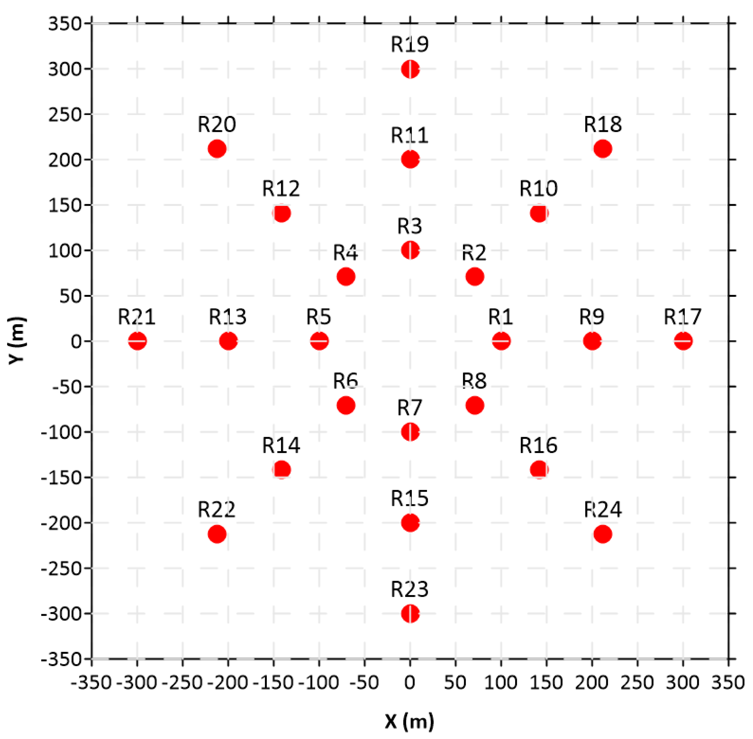
Figure 2.
Wind roses for year 2022 at Site 1 (a) and Site 2 (b).
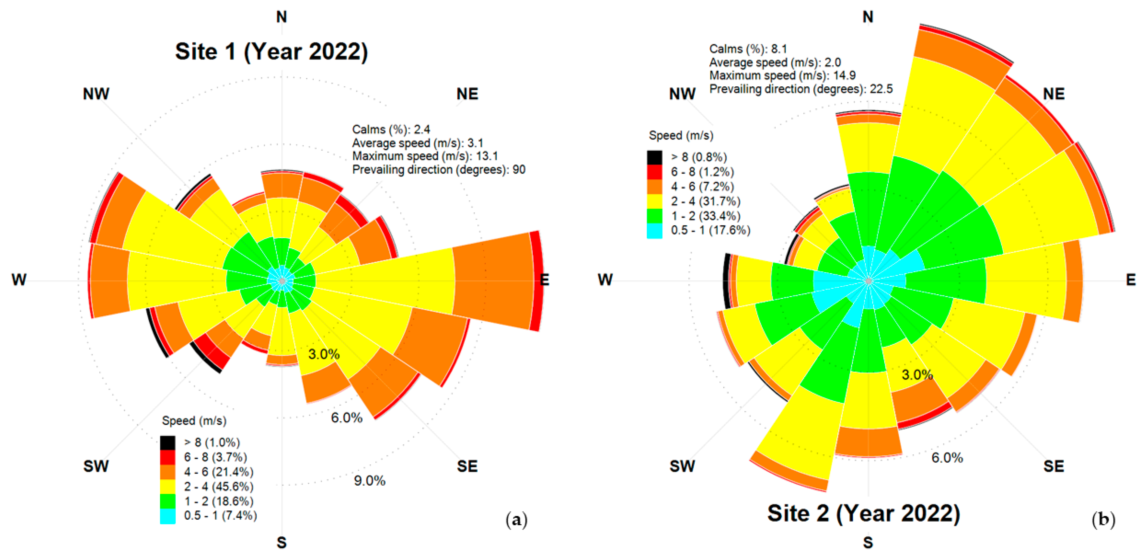
Figure 3.
Site 1. Scatter plot of the 98th percentile of hourly peak concentrations of LAPMOD versus CALPUFF for (a) vertical unobstructed stack and (b) rain capped stack.
Figure 3.
Site 1. Scatter plot of the 98th percentile of hourly peak concentrations of LAPMOD versus CALPUFF for (a) vertical unobstructed stack and (b) rain capped stack.
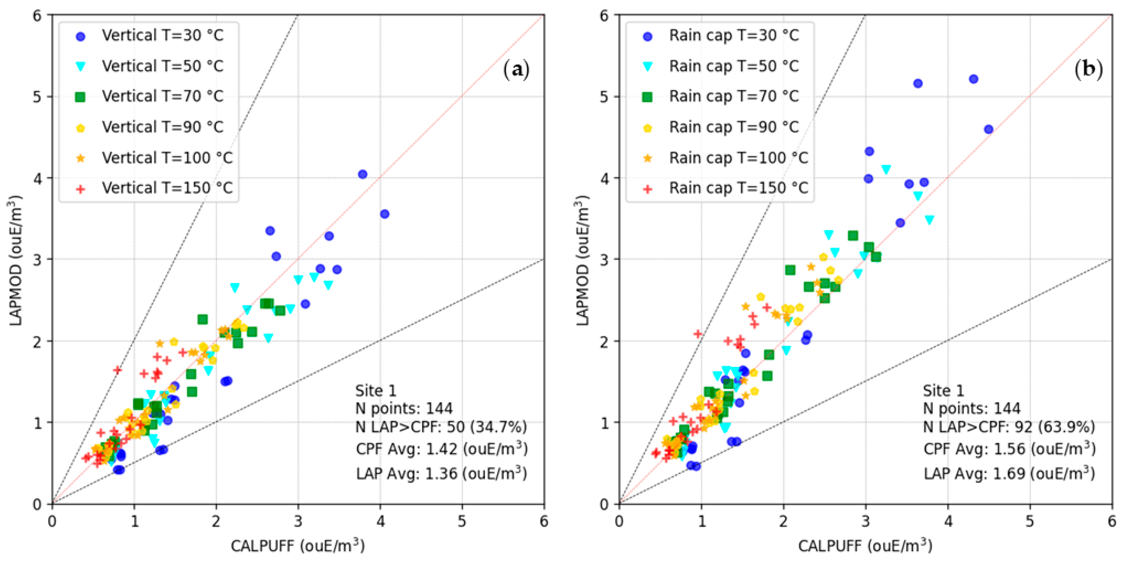
Figure 4.
Site 2. Scatter plot of the 98th percentile of hourly peak concentrations of LAPMOD versus CALPUFF for (a) vertical unobstructed stack and (b) rain capped stack.
Figure 4.
Site 2. Scatter plot of the 98th percentile of hourly peak concentrations of LAPMOD versus CALPUFF for (a) vertical unobstructed stack and (b) rain capped stack.
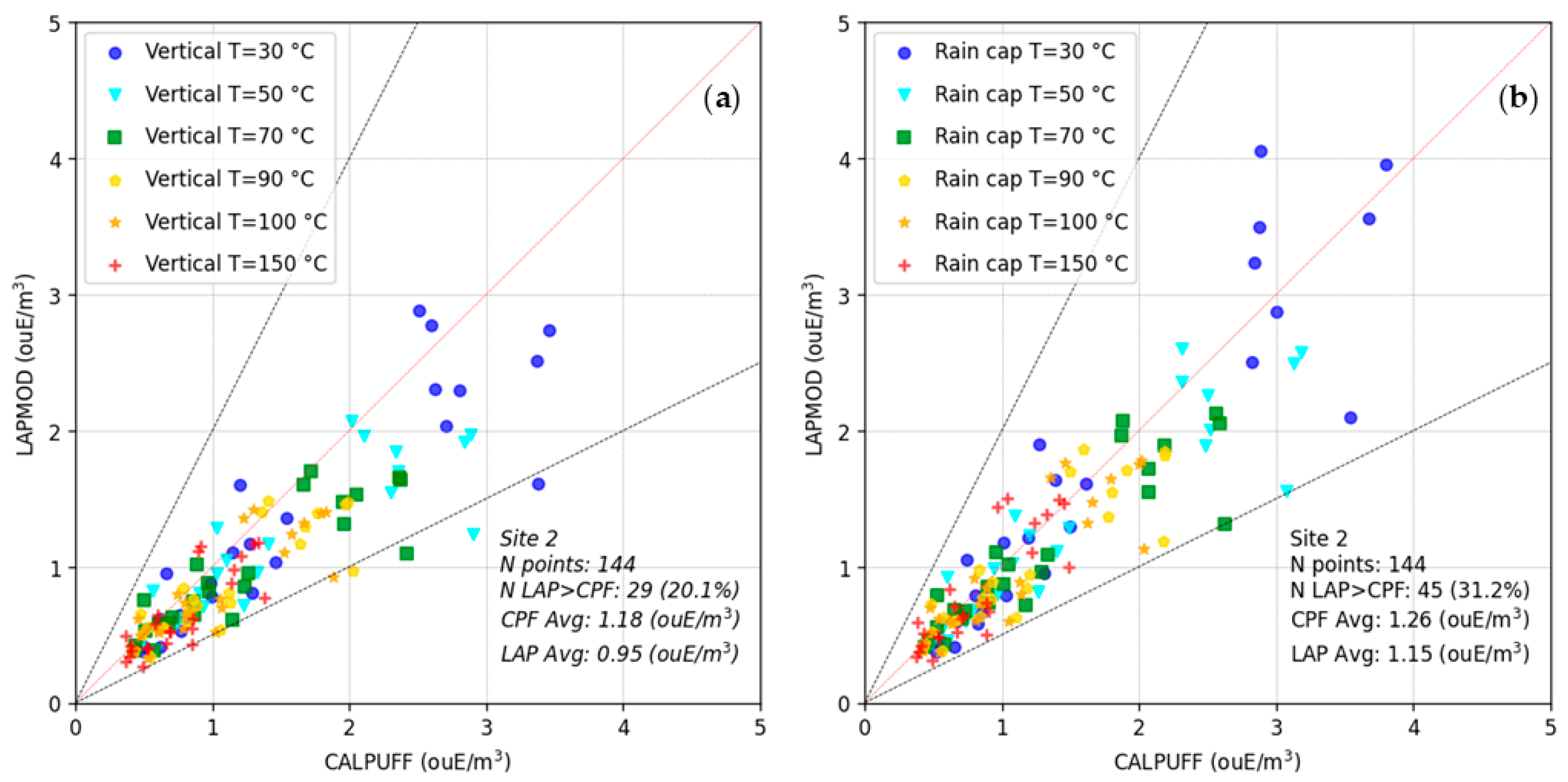
Figure 5.
Site 1. Scatter plot of the 98th percentile of hourly peak concentrations of LAPMOD versus CALPUFF for different emission temperatures: (a) T=30 °C, (b) T=50 °C; (c) T=70 °C; (d) T=90 °C; (e) T=100 °C; (f) T=150 °C. Vertical unobstructed stack.
Figure 5.
Site 1. Scatter plot of the 98th percentile of hourly peak concentrations of LAPMOD versus CALPUFF for different emission temperatures: (a) T=30 °C, (b) T=50 °C; (c) T=70 °C; (d) T=90 °C; (e) T=100 °C; (f) T=150 °C. Vertical unobstructed stack.
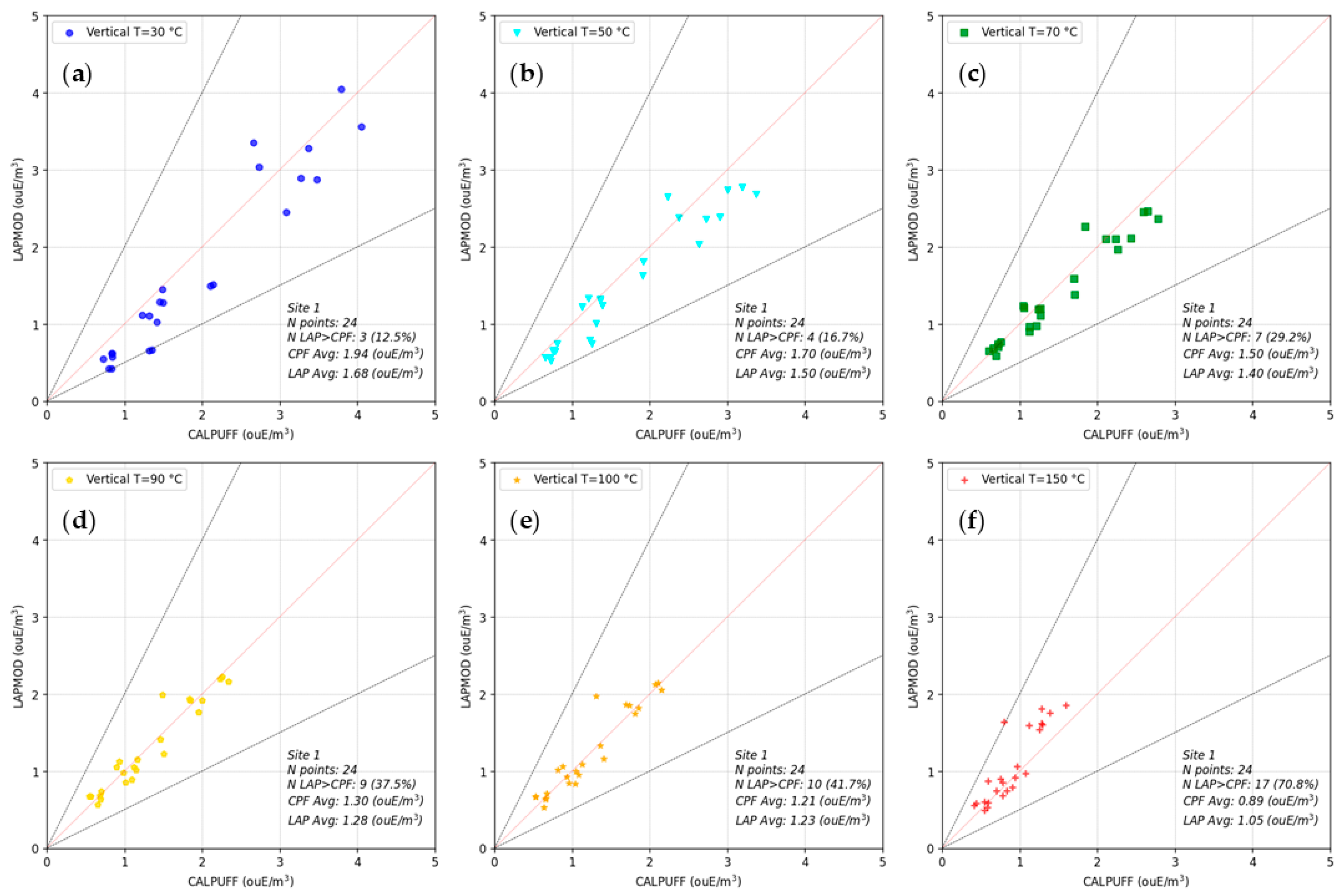
Figure 6.
Site 1. Scatter plot of the 98th percentile of hourly peak concentrations of LAPMOD versus CALPUFF for different emission temperatures: (a) T=30 °C, (b) T=50 °C; (c) T=70 °C; (d) T=90 °C; (e) T=100 °C; (f) T=150 °C. Vertical stack with rain cap.
Figure 6.
Site 1. Scatter plot of the 98th percentile of hourly peak concentrations of LAPMOD versus CALPUFF for different emission temperatures: (a) T=30 °C, (b) T=50 °C; (c) T=70 °C; (d) T=90 °C; (e) T=100 °C; (f) T=150 °C. Vertical stack with rain cap.
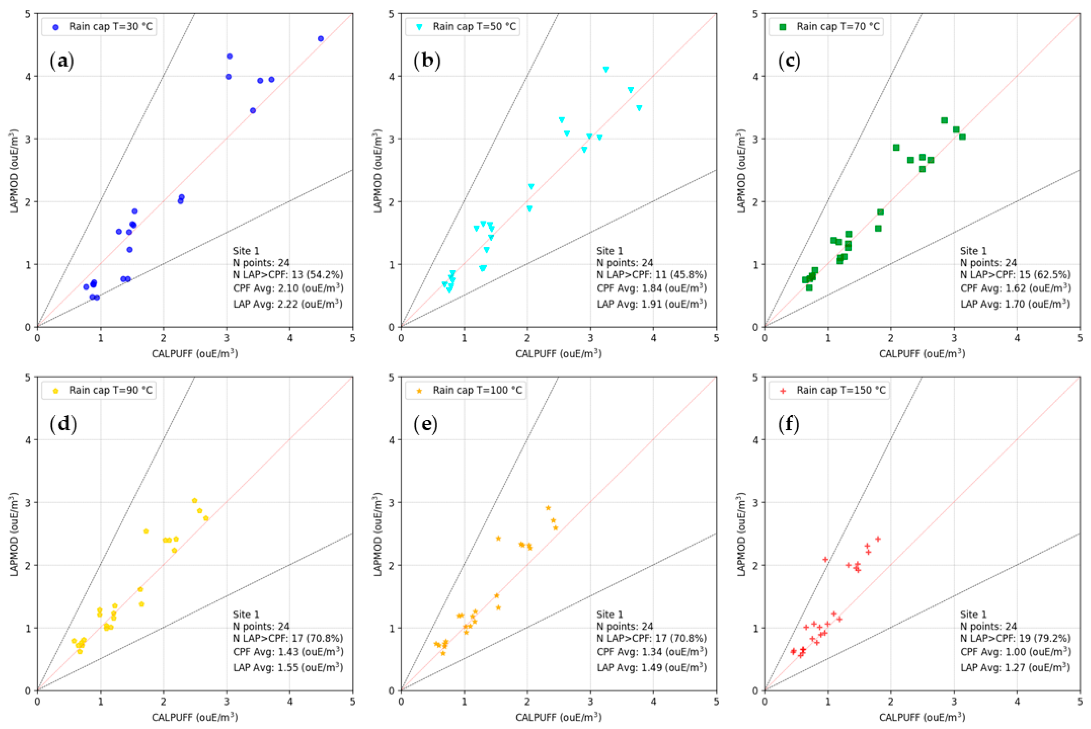
Figure 7.
Site 2. Scatter plot of the 98th percentile of hourly peak concentrations of LAPMOD versus CALPUFF for different emission temperatures: (a) T=30 °C, (b) T=50 °C; (c) T=70 °C; (d) T=90 °C; (e) T=100 °C; (f) T=150 °C. Vertical unobstructed stack.
Figure 7.
Site 2. Scatter plot of the 98th percentile of hourly peak concentrations of LAPMOD versus CALPUFF for different emission temperatures: (a) T=30 °C, (b) T=50 °C; (c) T=70 °C; (d) T=90 °C; (e) T=100 °C; (f) T=150 °C. Vertical unobstructed stack.
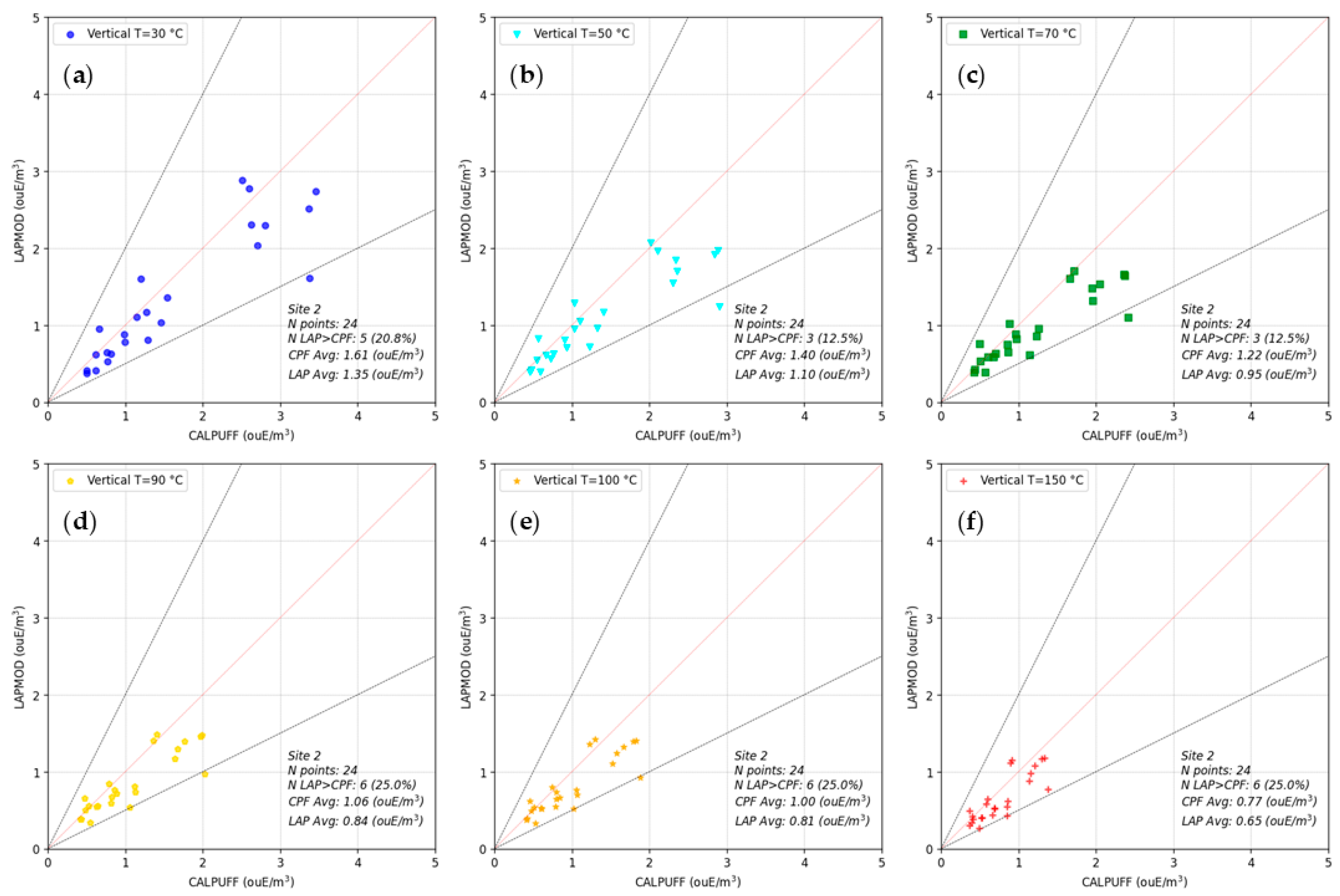
Figure 8.
Site 2. Scatter plot of the 98th percentile of hourly peak concentrations of LAPMOD versus CALPUFF for different emission temperatures: (a) T=30 °C, (b) T=50 °C; (c) T=70 °C; (d) T=90 °C; (e) T=100 °C; (f) T=150 °C. Vertical stack with rain cap.
Figure 8.
Site 2. Scatter plot of the 98th percentile of hourly peak concentrations of LAPMOD versus CALPUFF for different emission temperatures: (a) T=30 °C, (b) T=50 °C; (c) T=70 °C; (d) T=90 °C; (e) T=100 °C; (f) T=150 °C. Vertical stack with rain cap.
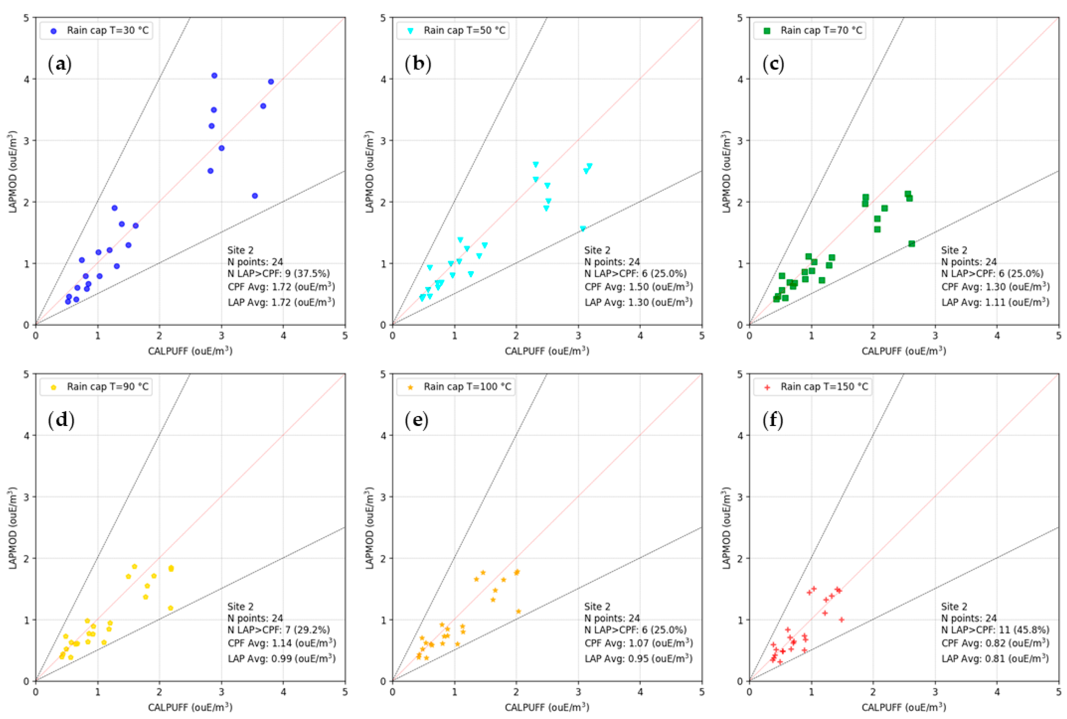
Figure 9.
Site 1. Scatter plot of the 98th percentile of hourly peak concentrations predicted by LAPMOD for different terminal types versus those predicted for a vertical unobstructed stack for different emission temperatures: (a) T=30 °C, (b) T=50 °C; (c) T=70 °C; (d) T=90 °C; (e) T=100 °C; (f) T=150 °C.
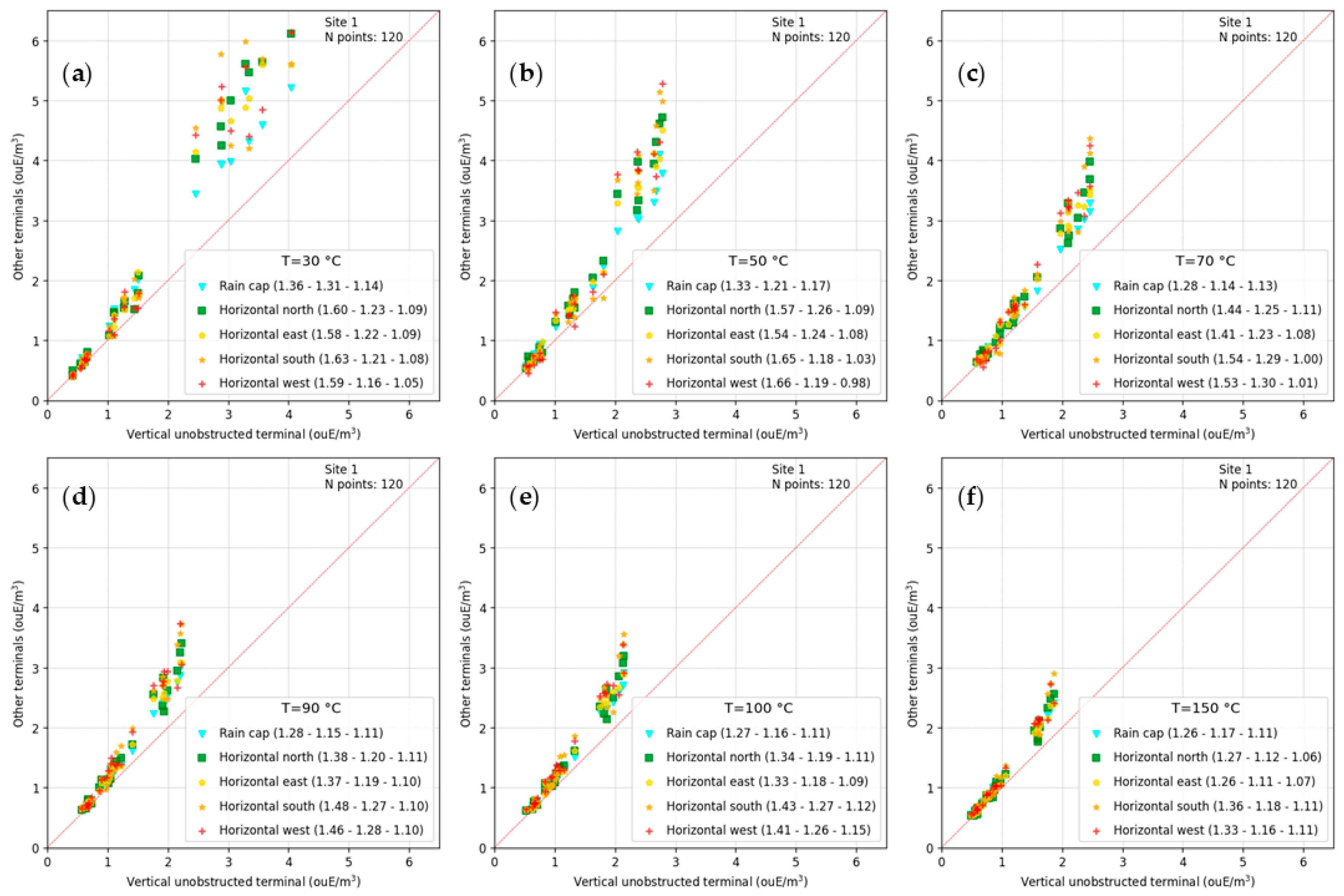
Figure 10.
Site 2. Scatter plot of the 98th percentile of hourly peak concentrations predicted by LAPMOD for different terminal types versus those predicted for a vertical unobstructed stack for different emission temperatures: (a) T=30 °C, (b) T=50 °C; (c) T=70 °C; (d) T=90 °C; (e) T=100 °C; (f) T=150 °C.
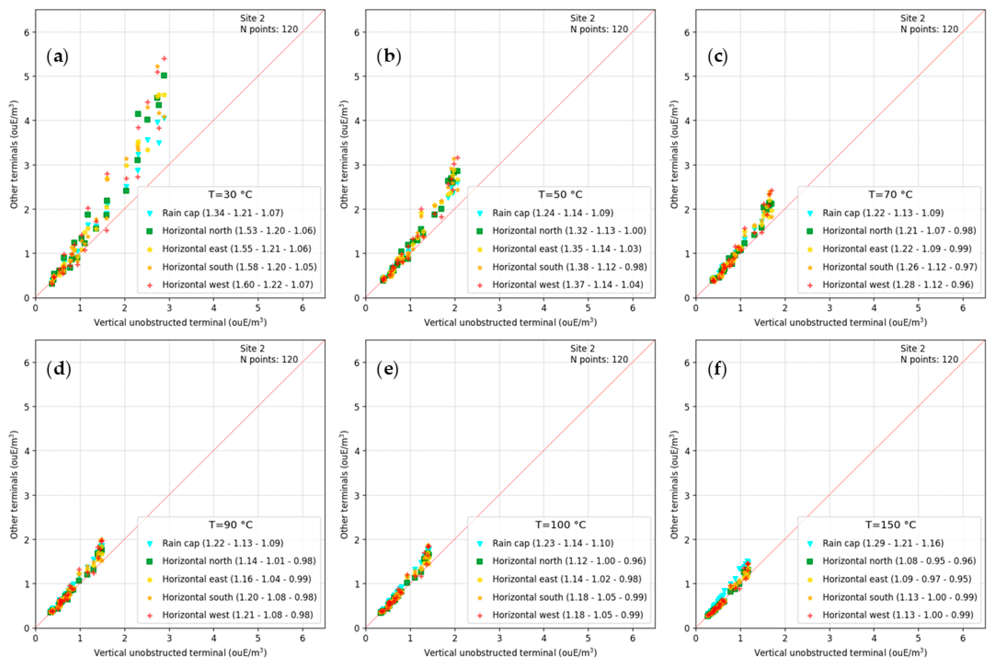
Figure 11.
Site 1. Examples of plume shapes in cold environment for an emission temperature of 30 °C and different terminal types: (a) vertical unobstructed; (b) rain capped; (c) horizontal pointing north; (d) horizontal pointing east; (e) horizontal pointing south; (f) horizontal pointing west.
Figure 11.
Site 1. Examples of plume shapes in cold environment for an emission temperature of 30 °C and different terminal types: (a) vertical unobstructed; (b) rain capped; (c) horizontal pointing north; (d) horizontal pointing east; (e) horizontal pointing south; (f) horizontal pointing west.
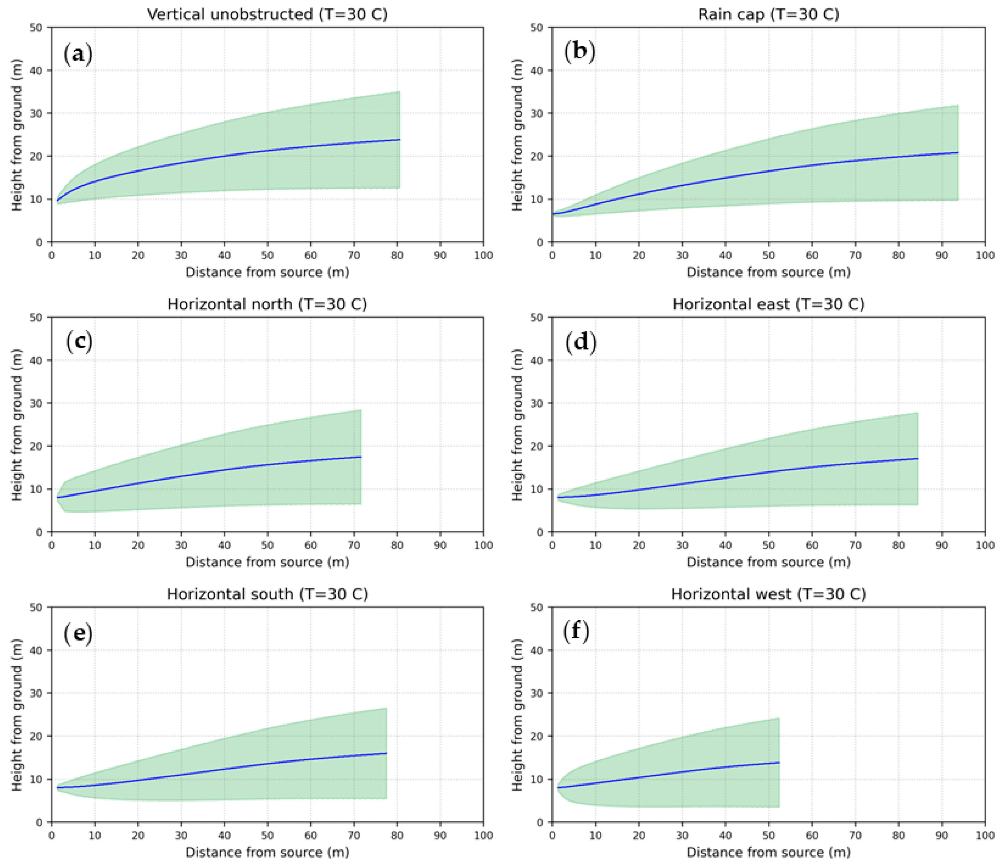
Figure 12.
Site 1. Examples of plume shapes in hot environment for an emission temperature of 30 °C and different terminal types: (a) vertical unobstructed; (b) rain capped; (c) horizontal pointing north; (d) horizontal pointing east; (e) horizontal pointing south; (f) horizontal pointing west.
Figure 12.
Site 1. Examples of plume shapes in hot environment for an emission temperature of 30 °C and different terminal types: (a) vertical unobstructed; (b) rain capped; (c) horizontal pointing north; (d) horizontal pointing east; (e) horizontal pointing south; (f) horizontal pointing west.
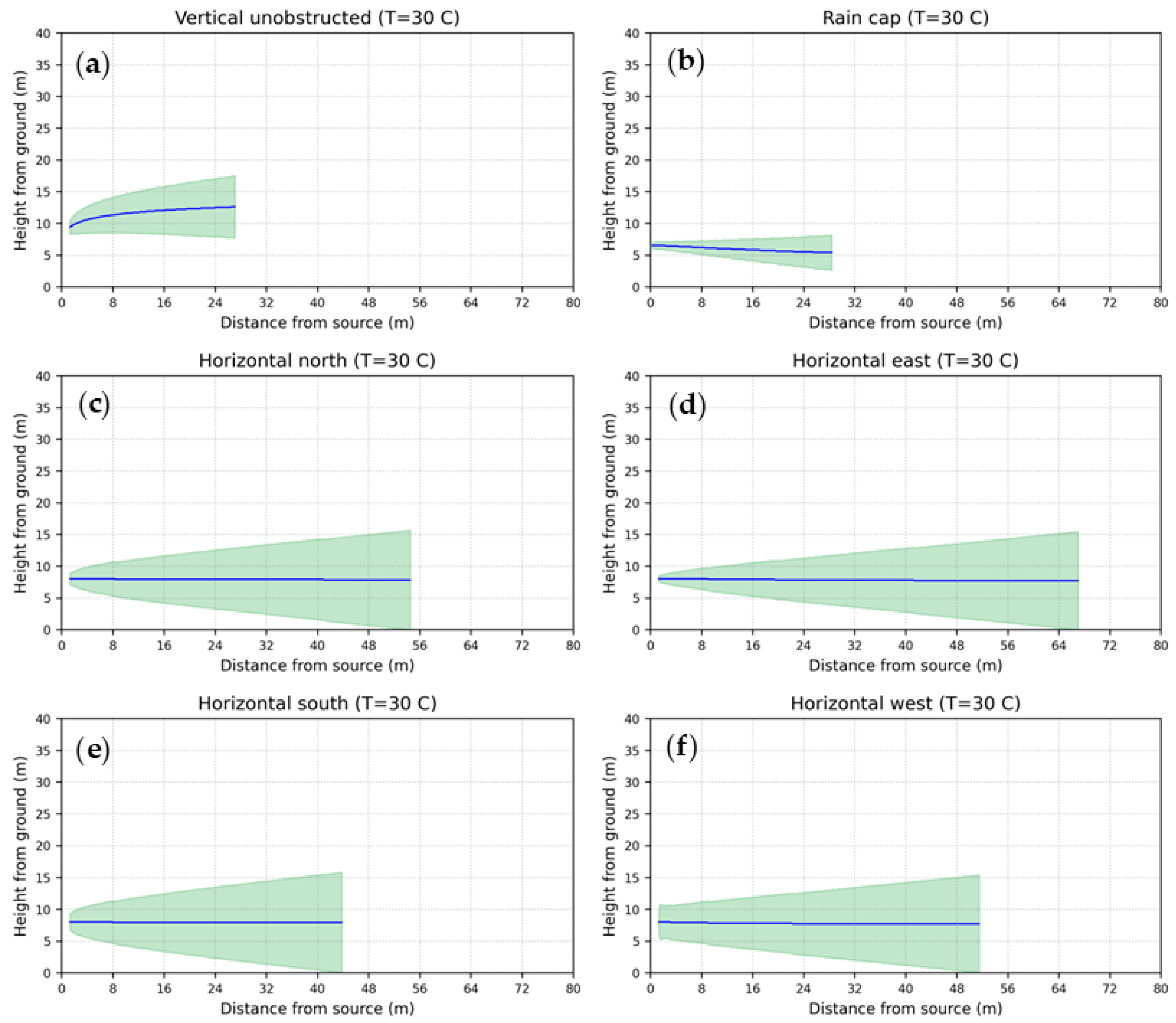
Figure 13.
Site 1. Examples of plume shapes in hot environment for a vertical unobstructed stack with different emission temperatures: (a) 30 °C; (b) 50 °C; (c) 70 °C; (d) 90 °C; (e) 100 °C; (f) 150 °C.
Figure 13.
Site 1. Examples of plume shapes in hot environment for a vertical unobstructed stack with different emission temperatures: (a) 30 °C; (b) 50 °C; (c) 70 °C; (d) 90 °C; (e) 100 °C; (f) 150 °C.
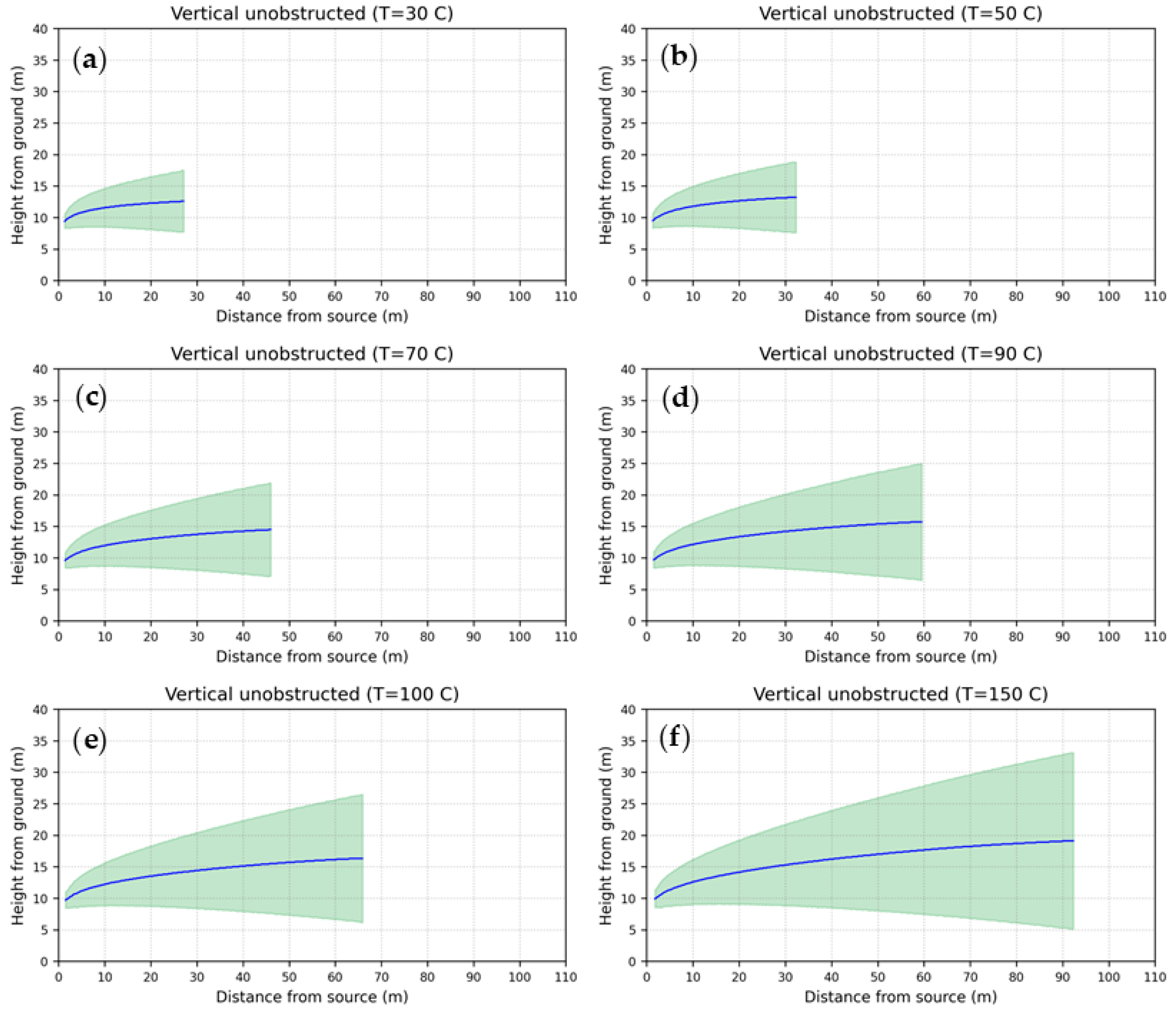
Figure 14.
Site 1. Examples of plume shapes in hot environment for a vertical rain capped stack with different emission temperatures: (a) 30 °C; (b) 50 °C; (c) 70 °C; (d) 90 °C; (e) 100 °C; (f) 150 °C.
Figure 14.
Site 1. Examples of plume shapes in hot environment for a vertical rain capped stack with different emission temperatures: (a) 30 °C; (b) 50 °C; (c) 70 °C; (d) 90 °C; (e) 100 °C; (f) 150 °C.
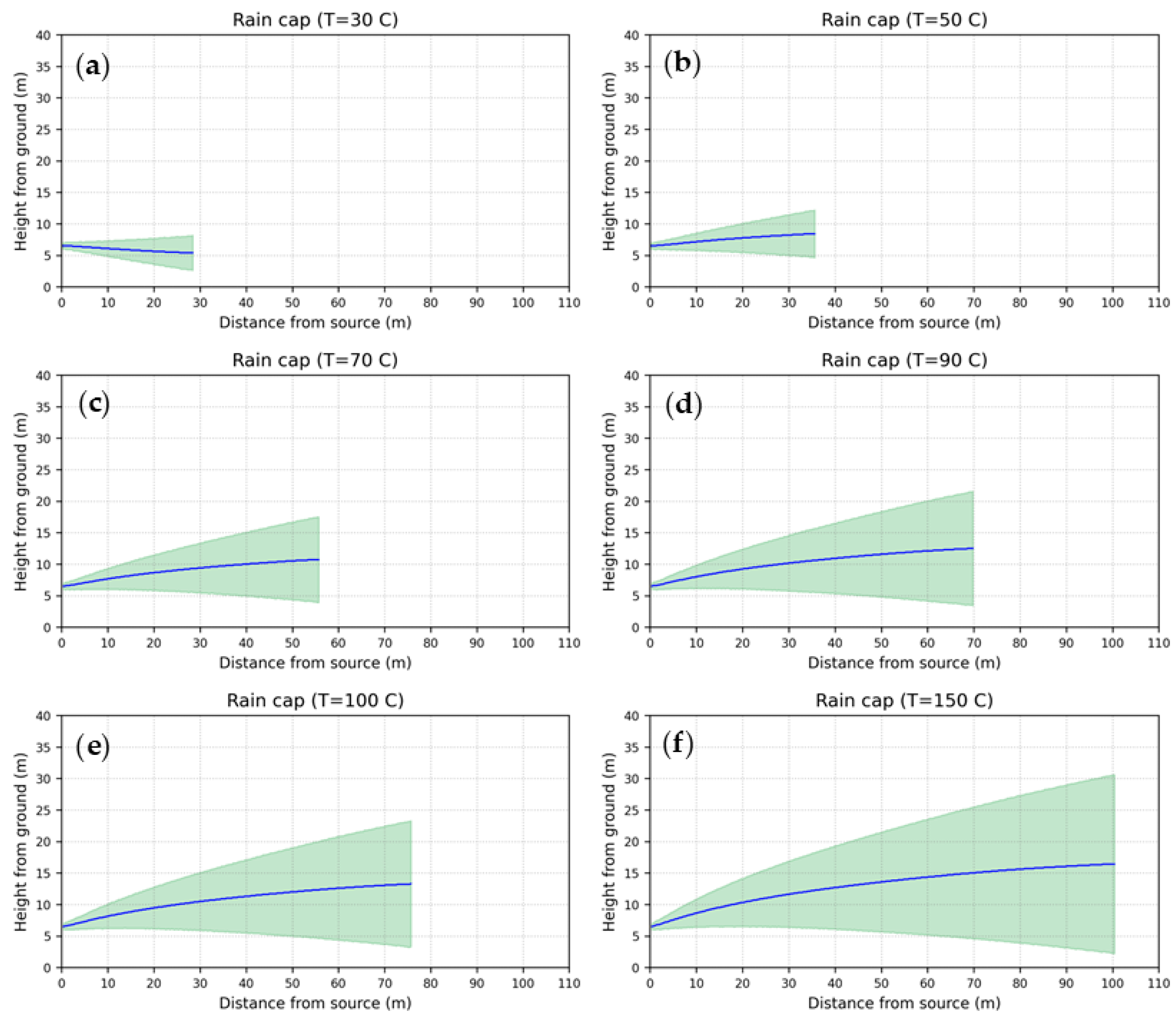

Table 1.
Source parameters.
| Parameter | Value | Units |
|---|---|---|
| Height | 8.0 | m |
| Diameter | 0.5 | m |
| Volumetric flow | 8000 | Nm3/h |
| Odor concentration | 4000 | ouE/m3 |
| OER | 9540 | ouE/s |
Table 2.
Exit temperatures and speeds.
| Temperature (°C) | Speed (m/s) |
|---|---|
| 30 | 12.6 |
| 50 | 13.4 |
| 70 | 14.2 |
| 90 | 15.0 |
| 100 | 15.5 |
| 150 | 17.5 |
Disclaimer/Publisher’s Note: The statements, opinions and data contained in all publications are solely those of the individual author(s) and contributor(s) and not of MDPI and/or the editor(s). MDPI and/or the editor(s) disclaim responsibility for any injury to people or property resulting from any ideas, methods, instructions or products referred to in the content. |
© 2025 by the authors. Licensee MDPI, Basel, Switzerland. This article is an open access article distributed under the terms and conditions of the Creative Commons Attribution (CC BY) license (http://creativecommons.org/licenses/by/4.0/).
Copyright: This open access article is published under a Creative Commons CC BY 4.0 license, which permit the free download, distribution, and reuse, provided that the author and preprint are cited in any reuse.


