
Submitted:
10 September 2025
Posted:
11 September 2025
You are already at the latest version
Abstract
The primary aim of this study is to develop an effective decision-support system for managing crises involving the release of hazardous airborne substances. Such scenarios often result from industrial accidents or intentional releases and require rapid contaminant source identification to facilitate timely response measures. This work focuses on a novel approach that integrates a modified Sandpile model with advection with the (1+1) Evolution Strategy to solve the inverse problem of source localisation. The initial part of the paper reviews existing methods for simulating atmospheric dispersion and reconstructing the source location. In the subsequent sections, we describe the proposed system architecture, modelling assumptions, and the experimental framework. A key feature of the presented method is that it relies solely on concentration measurements reported by a distributed network of sensors and does not require any prior knowledge about the source location, release time, or emission strength. The system was validated through a two-stage process using synthetic data generated by a Gaussian dispersion model. Preliminary experiments supported model calibration and refinement, followed by formal tests to evaluate localisation accuracy and robustness. Each test case was completed in under 20 minutes on a standard laptop, demonstrating the algorithm’s high computational efficiency. The results confirm that the proposed (1+1)-ES Sandpile model can effectively reconstruct source parameters within the resolution limits of the sensor grid. The system’s speed, simplicity, and exclusive reliance on sensor data make it a promising solution for real-time environmental monitoring and emergency response applications.
Keywords:
Sandpile model
; evolution strategy (1+1)
; optimisation process
; airborne contaminant source
; inverse methods
1. Introduction
The emission and storage of toxic substances pose a continuous risk of accidental or intentional release into the atmosphere, with potentially severe consequences for human health and the environment. Airborne pollution remains a key area of research due to its ability to affect large geographic areas and dense urban populations, especially when released materials are hazardous or difficult to detect. Such releases often result from uncontrolled leaks in industrial storage or transport systems. In other scenarios, they may be intentional and aimed at causing harm or public disruption. Regardless of the cause, early detection and characterisation of such events are critical to a timely and effective response. Sensor systems play a central role in the detection of airborne contaminants. Modern sensor networks, capable of measuring chemical concentrations in real time, are essential to identify the presence of toxic substances in the atmosphere. When integrated with atmospheric dispersion models, sensor data enable accurate tracking of contamination plumes and support source term estimation, namely identifying the release location, timing, and intensity. The most challenging and dangerous situations occur when elevated concentrations of an unknown contaminant are detected without prior information about its source. In such scenarios, rapid sensor data analysis combined with model-based inference can help estimate the release coordinates and emission rate. This capability is vital for initiating containment measures, issuing public safety alerts, and preventing the spread of hazardous materials.
The literature includes numerous papers focused on the location of the source of atmospheric contamination based on data collected from distributed sensors. The existing algorithms for this task can be categorised into two main types. The first type employs a backwards approach and is designed for open areas or continental-scale problems. The second type utilises a forward approach, where various parameters of a dispersion model, including the source location, are sampled to identify the one that minimises the distance between the model outputs and the measurements from the sensors within the specified spatial domain. This inverse problem does not have a unique analytical solution, but it can be analysed within probabilistic frameworks, such as the Bayesian approach, which treats all variables of interest as random variables (e.g., [1,2,3]). A comprehensive literature review of previous work that addresses the inverse problem of atmospheric contaminant releases can be found in sources such as [4].
Identifying the source of an atmospheric contaminant release is a computationally demanding task. Conventional methods require multiple simulations using complex dispersion models, where a single run can last from minutes to days. This computational burden is a significant obstacle in emergency scenarios that demand rapid source localisation based on sensor network data. Artificial neural networks have been proposed as an alternative to circumvent these long computation times, particularly in urban settings (e.g., [5,6]). However, successful source reconstruction depends not only on the dispersion model but also on an efficient algorithm for searching the parameter space to match model outputs with sensor measurements.
Various optimisation algorithms, including nature-inspired approaches, have been applied to this source reconstruction problem. Among recent developments is the Layered Algorithm, which employs a two-dimensional, three-state Cellular Automaton (CA) for classification [7]. This method categorises sensor measurements by magnitude into distinct data layers, enabling the CA to effectively identify the probable source location [8,9].
The Sandpile algorithm has also been explored for this application. A preliminary study proposed a simple model coupled with the Generalised Extremal Optimisation algorithm but crucially omitted the advection mechanism, limiting its physical realism [10].
In this paper, we continue this research by significantly expanding upon it and, most importantly, by introducing the advection mechanism. This enhancement allows our proposed model to more accurately represent real-world data. This study introduces a novel tool to identify the source of airborne contamination, using data collected from a distributed network of sensors. The proposed approach leverages the Sandpile model, traditionally used to simulate self-organised criticality, by adapting it to represent the transport and dispersion of airborne pollutants within a bounded spatial domain. The central aim is to explore the feasibility of applying the Sandpile model as a simplified yet effective method for simulating the movement of contaminants through the atmosphere.
The remainder of this paper is structured as follows. Section 2 presents the fundamentals of the Sandpile model and outlines the rationale for its application in the modelling of atmospheric pollution. Section 3 introduces the use of cellular automata to implement the simulation framework. Section 4 describes the (1+1)-Evolution Strategy ((1+1)-ES) algorithm, which is employed to optimise the source prediction process. Section 5 briefly discusses the concept of advection as a relevant transport mechanism. Section 6 provides an overview of the Gaussian dispersion model used to generate synthetic reference data for validation. Section 7 presents the simulation results and performance evaluation of the proposed method. Finally, Section 8 concludes the paper and outlines directions for future research.
2. Characteristic of the Sandpile Model
The Sandpile model is a well-known deterministic framework for studying self-organizing criticality. This model was proposed by Bak, Tang, and Wiesenfeld in 1987 (see, [11,12,13]). In this model, the steady-state (or critical state) eventually collapses at a certain point in time. The simplest version of the Sandpile model begins with a single column configuration. At each step, if a column contains at least two more grains than its right-hand neighbour, it will pass one grain to that neighbour. It has been proven (in [14,15]) that this model converges to a single configuration in which the evolution rule can no longer be applied to any column. This configuration is referred to as a fixed point. All possible arrangements that emerge from the initial column configuration through the application of the evolution rule can be characterised in the space of a two-dimensional grid [16].
To describe the Sandpile model, we can use a simple mental image involving rice [17]. Imagine a pile of sand on a small table. Dropping an additional grain onto the pile may trigger avalanches, causing grains to slide down the slopes. The dynamics of these avalanches depend on the steepness of the slope. As the avalanche occurs, the sand settles somewhere on the table. If the avalanche continues, some grains may fall off the edge of the table. On average, adding one grain to the pile will increase the slope. Over time, as the grains spread, the slope will evolve into a critical state. At this point, dropping a single grain into the pile can result in a large avalanche. This thought experiment illustrates that the critical condition is highly sensitive to stimuli; even a small change (whether internal or external) can lead to significant effects [18].
In the initial stage, we define a class of graphs on which the model is based. The graph G must be finite, undirected, connected, and loopless. It may contain multiple edges and include a distinctive terminal vertex. The set of graphs is denoted as G. The notation indicates adjacency in G, meaning .
The configuration of the Sandpile G model is represented by the vector . The number indicates the number of sand grains at the vertex in the configuration . When this number exceeds a certain threshold, the vertex is considered unstable and will distribute one grain of sand to each of its neighbours (see, Figure 1). The probability of a neighbouring vertex receiving a grain from an unstable vertex is drawn from the interval . The terminal vertex plays a special role, as it can accept an infinite number of grains and will never become unstable [12].
When the local slope of the stack—resulting from the height difference between the top and the adjacent vertex—exceeds a certain threshold, the grains will redistribute. This process allows one grain to fall onto another pile. It occurs by reducing one pile’s height while increasing adjacent piles’ height. In the subsequent iteration of pouring sand, the local threshold is recalibrated. This procedure continues until all vertices reach a stable configuration. At this point, a new grain is introduced from the left side. The configuration is considered stable when , where represents the degree of vertex in graph G [12,19].
In our study, we adopted an asynchronous sequential approach because seeds dropping at a single point can trigger an avalanche, which in turn induces changes at multiple points, ultimately leading to a stable state in the Sandpile Model in cellular automata (CA). During the avalanche, the sand seeds move down towards the base of the pile. However, if the seeds can fall in multiple directions, the direction is chosen with a probability proportional to the slope’s height in that direction.
The Sandpile Model is versatile and can be readily adapted to various research problems. It can exist in one or two dimensions with open, closed, or infinite boundaries. This model is widely employed in fields such as physics, economics, mathematics, and theoretical computer science [20,21,22,23,24]. Its applications range from cellular automata and information systems to earthquake calculations [25], studies of river sediments [26], the spread of forest fires [27], investigations of the Earth’s magnetosphere [28], studies of precipitation distribution [19], and diffusion problems (such as those involving Lattice-Gas and Lattice-Boltzmann models) [29].
3. Two-Dimensional CA Approach for Localisation Model
CAs and their potential for efficiently performing complex computations were described by S. Wolfram in [30]. This paper focuses on two-dimensional CA. A cellular automaton is represented as a rectangular grid of cells, where each cell can assume one of k possible states. After establishing the initial states of all cells (that is, the initial configuration of the cellular automaton), each cell updates its state according to a transition function , which is based on the states of neighbouring cells.
In this study, a finite cellular automaton with stable boundary conditions is utilised. The transitions between states of the CA occur asynchronously. The transition function employed in this paper is derived from the Sandpile model, applied to the cellular automaton grid. In this context, the cellular automaton cells simulate the sand grains’ evolution in the Sandpile model.
Assuming that the contaminant distribution domain extends over the region (in meters), the data space must be mapped from to the grid of cells. For simplicity, this paper assumes a square grid with (see, also [10]).
4. Localisation Model Based-on the (1+1)-ES-Sandpile Model
Evolution strategies (ES) are one of the four main categories of evolutionary algorithms. A distinctive feature of ES is its specific approach to adapting the mutation step size. If new solutions do not improve upon previous ones, the algorithm dynamically adjusts the mutation range. Another characteristic of ES is that a well-adapted individual can pass on to the next generation without modification.
Evolution strategies are divided into several types (see, [31,32,33,34,35]). One example is the (1+1)-ES, which creates a single offspring from one parent, selecting the better-adapted individual to proceed to the next generation, as shown in Algorithm 1. Over time, new variants of evolution strategies have emerged, such as the () and () strategies. These types are primarily used for problems where the encoding can be easily represented as a vector of floating-point numbers.
The Algorithm 1 presents the for the Evolution strategy (1+1) procedure. The is the mutation range parameter and is the normal distribution. The is the self-adaptive mutation range algorithm shown in Algorithm 2.
| Algorithm 1 Evolutionary strategy (1+1) |
|
| Algorithm 2 Self-adaptive mutation range algorithm for evolutionary strategy (1+1) |
|
The , in Algorithm 2 are parameters having values: and . The success rule, denoted as , and its corresponding value were first proposed by Rechenberg following his studies on multidimensional functions. The scaling factors used to adjust the size of the mutation step—specifically to increase () or decrease () the step—were experimentally derived and are standard recommendations by Schwefel (see [36]).
In the (1 + 1) Evolution Strategy algorithm, the fitness function is computed as the sum of the relative differences between the results of the Sandpile model and the contaminant concentrations at sensor locations. The difference at each point is calculated using the following formula (based on [10,37]):
where: is the concentration value at the j-th sensor location, is the concentration value estimated by the Sandpile model at the j-th sensor location, N is the total number of sensors.
If the output of the Sandpile model is equal to 0, it is assumed to be to facilitate the logarithm calculation. The final evaluation function is the sum of the differences from all sensor positions considered. The evaluation function tends toward a minimum; thus, a smaller value of the obtained difference indicates a better match between the Sandpile model and the target concentrations at the sensors.
The (1+1) evolution strategy is quite sensitive to local minima, which has prompted the search for more effective solutions. This search has led to the development of various strategies, including , , and .
In all these strategies, individuals are represented by a pair of vectors: X and . The solution vector represents an individual within an n-dimensional solution space. The mutation step-size vector contains values where is used to mutate the gene , with j ranging from 1 to n.
In each strategy, the mutation process affects both vectors. First, the step-size vector is mutated using the parameters and (as detailed in Algorithm 2). After this adjustment, the solution vector X is mutated using the newly modified step-size (as outlined in Algorithm 1).
5. Advection in the Sandpile Model
In the basic Sandpile model, a point is selected for the addition of successive grains of sand. When a grain falls from a certain height, its trajectory is a straight line from the release point to the top of the grain column located directly beneath it.
In this enhanced version proposed in the paper, wind advection emerges as a significant factor influencing the trajectory of falling grain. The ultimate landing position of the grain is precisely determined by mathematical equations that capture the dynamics of particle movement in the air. In this context, the speed and direction of the wind are pivotal, underscoring their critical role in shaping the grain’s descent and relocation.
Figure 2 presents a conceptual diagram of a sand grain’s trajectory as it falls under the influence of wind. A red dot indicates the release point, while the green path and cell show where the grain would land without wind. The blue line represents the wind flow, and the yellow path illustrates the grain’s trajectory influenced by the wind, along with the final target cell.
Our model, developed within our system, utilises a cellular automaton approach. Each cell in the grid represents the height of a grain pile, which is determined by the number and size of the grains it contains. When a grain falls onto the peak of a column at coordinates , we check its four neighbouring cells: , , , and .
If the height difference between the selected peak and any of its neighbours is no more than three grains, the grain remains at the current peak, and its height increases by the size of the new grain. However, if the height difference between the selected peak and a neighbouring cell equals the height of four grains, a neighbouring peak is randomly chosen for the grain to slide onto. During this process, neighbouring peaks that are the same height or higher are excluded from selection. The probability of a grain sliding onto a selected neighbour increases with the height difference. This cascading movement continues recursively until all grain columns reach a stable state.
The model’s parameters include the coordinates of the grid’s starting point and height, as well as the direction and speed of the wind, which influence the movement of the falling grains. The formula used to calculate the height of a grain at given coordinates, taking into account the wind direction and speed, is as follows:
where:
- z — the height of a grain at coordinates ,
- h — the height of the grain release point,
- g — acceleration due to gravity (),
- — cell coordinates,
- — the scale of the cellular automaton with respect to coordinates X and Y,
- — wind gradient as a vector , where ,
- — wind speed in .
During the simulation, the altitude of a grain particle is determined using the wind direction gradient for cells within the particle’s trajectory. If the particle’s altitude in the next cell is lower than or equal to the altitude of existing grain vertices in that cell, or if it falls below the grid (i.e., ), the particle is deposited onto the vertex in the current cell. For example, if a particle is over cell and the wind gradient indicates that it will move to cell , we calculate the particle’s altitude above this new location. If this altitude is less than or equal to the vertex height at , or if it is below zero, the particle will be deposited at the vertex of the current cell . A typical outcome from our model is shown in the left panel of Figure 4.
6. Assessing the Suitability of the (1+1)-ES Sandpile Model for Airborne Contaminant Source Localization
6.1. Generation of Synthetic Data for Model Evaluation
This chapter examines the applicability of the (1+1)-ES-Sandpile model to the problem of airborne contaminant source localisation. To assess the performance of the proposed approach, synthetic concentration data were generated over the simulation domain using the well-established Gaussian dispersion model (e.g., [39]). This controlled setup enables a systematic evaluation of the algorithm’s ability to identify the source location under simplified yet representative atmospheric conditions.
The Gaussian plume model remains one of the most widely used approaches in air pollution studies. It provides a simplified analytical representation of the three-dimensional concentration field produced by a continuous point source under stationary meteorological and emission conditions. Although it relies on several simplifying assumptions, the model is still commonly applied due to its robustness and ease of use. Under uniform and steady wind conditions, the concentration of a contaminant (in ) at a location defined by meters downwind of the source, meters laterally from the plume centerline, and z meters above ground level can be expressed as:
where U denotes the wind speed along the x-axis, Q is the source strength or emission rate, and H is the effective release height, defined as the sum of the physical release height and the plume rise h (). The dispersion parameters and , representing the standard deviations of the concentration distribution in the crosswind and vertical directions, respectively, are empirical functions of and depend on atmospheric stability conditions as defined by Pasquill and Gifford (e.g., [39]).
A Gaussian dispersion plume model was used to generate a map of the spread of the contaminant in a specific area. We limited the diffusion to stability class C for the urban environment (using Pasquill type stability for rural areas). The release rate was assumed to vary over time within the range , which caused changes in the concentration recorded by the sensors in subsequent time intervals. The wind was directed along the x-axis, with an average speed of .
The spatial distribution of the contaminant within the simulation domain is shown in Figure 3. A corresponding sample of the contaminant field, mapped onto the computational grid, is presented in the right panel of Figure 4. For this purpose, the physical domain m was discretised into a grid, which served as the input representation for the (1+1)-ES-Sandpile model.
Figure 4 shows that the contaminant distributions generated by both the Gaussian plume model and the Sandpile model with the right parameter configuration are nearly identical. This similarity is consistent with the expected behaviour of the Sandpile model when advection properties are applied with the same parameters. The results suggest that the Sandpile model is a promising tool for estimating Gaussian distributions and, by extension, for modelling airborne contaminant dispersion. Furthermore, subsequent experiments demonstrate the effectiveness of our advection-enhanced Sandpile model in reconstructing the source location of the substance’s release.
6.2. Testing Framework and Assumptions
The (1+1)-Evolution Strategy (ES) Sandpile model, described in detail in Section ??, was evaluated for its efficiency in localising a contamination source using synthetic sensor data generated by the Gaussian plume model (Section 3).
The concentrations reported by the sensor grid were fed into the (1+1)-ES algorithm to determine whether it could accurately identify an airborne contaminant source within the specified domain. The (1+1)-ES algorithm was applied to the Sandpile model, utilising a two-dimensional cellular automaton (CA) of size . A larger CA size is expected to produce more accurate results, contingent upon a denser data grid. The number of sand grains () used in this model ranged from 0 to grains, while the grain size () varied from 0 to 1 meter. Wind direction and speed were represented by the vector . The algorithm ran for 200 generations.
In this context, an individual is represented by a pair of vectors . The solution vector X is defined as , while represents the mutation step-size vector of the (1+1)-ES algorithm. Here, and Z denote the positions where grains of sand are dropped, and indicate the wind parameters, is the number of grains, and is the grain size. Each value of falls within the range . Each experiment was conducted with 10 restarts.
7. Evaluation Results of the (1+1)-ES Sandpile Source Localization Model
Our research was structured in two sequential stages to address the problem’s complexity. The initial stage focused on an inverse problem: fitting the Sandpile model’s parameters to match the contaminant distributions reported by a network of sensors. This calibration process was essential to validate the model’s ability to accurately simulate real-world plumes. The second stage then leveraged this validated model to pinpoint the source characteristics, testing its efficacy by using the simulated plumes to reconstruct the original release location.
7.1. Adjusting the parameters of the Sandpile model to align with sensor data.
The first and most crucial stage involves experimentally adjusting the parameters of the Sandpile model to match the contaminant spread reported by the sensor network. A well-fitted Sandpile model will enable the identification of the release point in the second stage of the process.
Two groups of testing data were utilised. The first set was employed for preliminary tests (the first stage of experiments). This set comprises readings of contaminant concentration measured across a regular grid of sensors, with one sensor allocated to each square kilometer. The test domain was a square measuring 10 km by 10 km, containing 100 regularly spaced sensors arranged in a 1 km grid, positioned 2.5 m above the ground. The contaminant source was situated within the domain at the coordinates (0 m, 5000 m) and was 28.75 m above the ground. The emission rate was set at , with the wind blowing parallel to the x-axis at a speed of . A visualisation of the simulation results from the Gaussian model contained in this data set is shown in Figure 5.
In line with the assumptions and experimental plan, it was necessary to estimate the appropriate grain size and the correct number of grains to be dispensed. The results of the tests are presented in the tables below, considering all parameters of the Sandpile model.
The (1+1)-ES Sandpile model was executed to estimate the number of grains and the grain size , while keeping the other parameters at the following levels: , , and . The number of generations applied in the algorithm was equal to 200. The results presented in Table 1 are sorted from the best fit to the worst.
The objective is to minimise the function , where a value of 0 indicates a perfect fit of the Sandpile model to the contaminant spread reported by the sensor network. As shown in Table 1, the best score was obtained with a grain size and a large number of grains (the first row in Table 1), yielding an evaluation function . The last row of the table indicates that with a grain size that is too large, specifically , only a small number of grains were dispensed to fit the model, resulting in a poor fit (high evaluation function).
Despite these results, the high value of the evaluation function suggests that the models did not achieve a good fit. Therefore, tests were conducted on the Z-coordinate, which had not been previously mapped to the simulation coordinates, such as the CA grid in the Sandpile model. Subsequent experiments were carried out to determine the optimal height from which to pour the sand grains. In these experiments, we analysed and identified as the selected value, with an evaluation function of .
The goal of the first step of the experiments was to fit the Sandpile model to the sensor data, to propose a dispersion model that matches the registrations as much as possible. As a result, we selected the parameters that yielded the best results using the (1+1)-ES algorithm, which approximated the Sandpile parameters as follows: height of dropping seeds , grain size , and number of grains .
7.2. Determining the Location of an Airborne Contaminant Source
The parameters of the Sandpile model selected in the previous stage of the algorithm were used to conduct tests on five different datasets. These datasets represented the concentration of the released substance in a sensor grid, with random source locations within the specified domain (see, Figure 6).
In the datasets used in this section to evaluate the effectiveness of the proposed algorithm for contaminant source localisation, the release height varied across scenarios (see, Figure 6). As a result, the previously fixed sand-dumping height parameter, (see, Section 7.1), was treated as a variable to be estimated alongside the horizontal source coordinates . The (1+1)-ES algorithm was employed in the following experiments to estimate the contaminant source position within the domain. The algorithm’s constant parameters were set as follows: grain size , number of scattered grains , and wind conditions . The objective was to accurately determine the source location . The results of these experiments are summarised in Table 2.
Table 2 presents a comparison between the true coordinates of the source of the contaminant and those estimated by the (1+1) ES Sandpile algorithm in five test cases. The algorithm demonstrates strong performance in estimating the horizontal source location, with most predicted X and Y values closely matching the true coordinates. Although some larger deviations appear, particularly in Cases 4 and 5, these fall within the expected accuracy range of approximately 1000 meters, which corresponds to the sensor spacing in the input grid. This suggests that the observed horizontal errors are largely attributable to grid resolution rather than algorithmic limitations. For vertical estimation, the algorithm shows a tendency to overestimate the release height. This behaviour can be explained by the intrinsic characteristics of the sandpile model. In the sandpile analogy, sand particles are released from a specific height, with their size and number directly influencing the resulting distribution pattern. In contrast, when generating testing datasets of airborne contaminants using the Gaussian model, the physical weight of the particles is not explicitly considered in the same way. As a result, the analogy between the two processes introduces a systematic bias in the estimated release height, making the Z coordinate slightly less precise compared to the horizontal ones. Nevertheless, this tendency is consistent across test cases, which suggests that it can be accounted for and potentially corrected in future refinements of the approach.
Overall, the (1+1)-ES Sandpile algorithm provides reliable and practically meaningful estimates of contaminant source locations, particularly in the horizontal plane, making it a promising approach for environmental monitoring applications.The absolute errors for each coordinate are summarized in Table 3, supporting these observations.
It is important to highlight the computational efficiency of the proposed algorithm. Each test case run on a standard laptop configuration was completed in under 20 minutes, which is significantly faster than many traditional inverse modeling approaches. This level of responsiveness is crucial in practical applications, where timely information is essential for effective decision-making. In emergency scenarios involving hazardous releases or environmental contamination, generating accurate source estimates within such short time frames can greatly improve the speed and effectiveness of response efforts. These results demonstrate the algorithm’s strong potential as a near-real-time solution for operational use in emergency management and environmental monitoring.
8. Conclusions
In a world facing the ongoing threat of airborne contaminants, this study introduces a novel approach to a critical issue: the rapid localisation of an unknown source. By adapting the well-established Sandpile model, which is traditionally used to simulate self-organised criticality, we have demonstrated its potential as a computationally efficient tool for modelling atmospheric dispersion. This work successfully integrates the Sandpile model with the (1+1) Evolution Strategy (ES), creating a robust framework for solving the inverse problem of source term estimation. Using synthetic data generated by the well-established Gaussian dispersion model, our two-stage validation process yielded highly promising results.
- Model Accuracy: We demonstrated that our advection-enhanced Sandpile model accurately reproduces the contaminant concentration fields generated by the Gaussian model. This finding confirms that the simplified Sandpile approach can effectively capture the complex physics of atmospheric transport and dispersion. As shown in Figure 7, the heat maps of contaminant distribution from both models are nearly identical, validating the Sandpile model as a viable alternative to more complex simulations.
- Localisation Performance: The (1+1)-ES Sandpile model proved to be highly effective at solving the inverse problem of source localisation. Using only the sensor data as input, our proposed framework identified the source coordinates with acceptable accuracy. The algorithm’s ability to converge on the correct solution with minimal computational overhead highlights its superiority for emergency response applications, where time is critical. Our experiments demonstrated that the model can accurately pinpoint the source, showcasing its practical utility for crisis management.
- Computational Efficiency: A key outcome of this research is the significant reduction in computational time compared to traditional multi-run dispersion models. Using the Sandpile model as a fast-forward simulator, we quickly iterated through potential solutions with the (1+1)-ES. This approach is well-suited for real-time applications, where a rapid and accurate response is essential for public safety.
Future work should focus on incorporating more complex meteorological and environmental factors, such as atmospheric turbulence, wind shear, and variable terrain, to further enhance the model’s accuracy.
References
- Kopka, P.; Wawrzynczak, A. Framework for stochastic identification of atmospheric contamination source in an urban area. Atmos. Environ. 2018. [Google Scholar]
- Wawrzynczak, A.; Kopka, P.; Borysiewicz, M. Sequential Monte Carlo in Bayesian assessment of contaminant source localization based on the distributed sensors measurements. Lecture Notes in Computer Sciences, 2014. [Google Scholar]
- Borysiewicz, M.; Wawrzynczak, A.; Kopka, P. Stochastic algorithm for estimation of the model’s unknown parameters via Bayesian inference. In Proceedings of the Federated Conference on Computer Science and Information Systems, Wroclaw, Poland, 9-12 September 2012; IEEE Press: Wroclaw, Poland, , 501–-508, 2012. [Google Scholar]
- Hutchinson, M.; Oh, H.; Chen, W. H. A review of source term estimation methods for atmospheric dispersion events using static or mobile sensors. Inf. Fusion.
- Wawrzynczak, A.; Berendt-Marchel, M. Can the artificial neural network be applied to estimate the atmospheric contaminant transport? Advances in High Performance Computing: Results of the International Conference on High Performance Computing Borovets, Bulgaria, 2019; Dimov, I., Fidanova, S., Eds.; Springer Nature: Cham, Switzerland, 2021. [Google Scholar]
- Wawrzynczak, A.; Berendt-Marchel, M. Computation of the airborne contaminant transport in urban area by the artificial neural network. Comput. Sci. ICCS 2020: 20th International Conference, Amsterdam, The Netherlands, June 3-5, 2020, Proceedings, Part II; Krzhizhanovskaya, V. V., et al., Eds.; Springer Nature: Amsterdam, The Netherlands, 2020. [Google Scholar]
- Szaban, M.; Wawrzynczak, A. 2022; -9.
- Szaban, M.; Wawrzynczak, A. , The Algorithm of Area Optimization by Layers and Binary Classification with Use of Three State 2D Cellular Automata, Proceedings of the International Conference on Control, Artificial Intelligence, Robotics and Optimization, ICCAIRO 2018, 283 - 288.
- Szaban, M.; Wawrzynczak, A. , Testing the Algorithm of Area Optimization by Binary Classification with Use of Three State 2D Cellular Automata in Layers, Annals of Computer Science And Information Systems, Proceedings of the 2018 Federated Conference on Computer Science and Information Systems, 15, 2018, 81 – 84.
- Szaban, M.; Wawrzynczak, A.; Berendt-Marchel, M.; Marchel, L. Application of the Generalized Extremal Optimization and Sandpile Model in Search for the Airborne Contaminant Source, In: Malyshkin, V. (eds) Parallel Computing Technologies, PaCT 2021, LNCS 12942, Springer, Cham. 2021. [Google Scholar]
- Bak, P.; Tang, C.; Wiesenfeld, K. Self-organized criticality: An explanation of the 1/f noise. Phys. Rev. Lett. 59(B11).
- Chan, Y.; Marckert, J. F.; Selig, T. A natural stochastic extension of the sandpile model on a graph. J. Comb. Theory Ser. A, 2013. [Google Scholar]
- Himangsu, B.; Santra, S. B. Stochastic sandpile model on small-world networks: Scaling and crossover. Physica A, 2018. [Google Scholar]
- Goles, E.; Morvan, M.; Phan, H. D. Sandpiles and order structure of integer partitions, Discrete Appl. Math., 117, 2002, 51–64.
- Latapy, M.; Mataci, R.; Morvan, M.; Phan, H. D. Structure of some sandpiles model. Theoret. Comput. Sci. 2001. [Google Scholar]
- Formenti, E.; Pham, T. V.; Duong Phan, T. H.; Thu, T. Fixed-point forms of the paralel symmetric sandpile model. Theoret. Comput. Sci. 2014. [Google Scholar]
- Frette, V.; Christensen, K.; Malthe-Sørenssen, A.; Feder, J.; Jøssang, T.; Meakin, P. Avalanche dynamics in a pile of rice. Nature, 1996. [Google Scholar]
- Hesse, J.; Gross, T. Self-organized criticality as a fundamental property of neural systems. Front. Syst. Neurosci.
- Aegerter, C. M. A sandpile model for the distribution of rainfall? Physica A 2003, 319, 1–10. [Google Scholar] [CrossRef]
- Parsaeifard, B.; Moghimi-Araghi, S. Controlling cost in sandpile models through local adjustment of drive. Physica A, 2019. [Google Scholar]
- Bjorner, A.; Lovasz, L.; Shor, W. Chip-firing games on graphs. European J. Combin. 12.
- Bak, P. How Nature Works: The Science of Self-Organized Criticality, 1st ed.; Springer: New York, NY, USA, 1999. [Google Scholar]
- Latapy, M.; Phan, H. D. The lattice structure of chip firing games. Physica D, 2000. [Google Scholar]
- Rossin, D.; Cori, R. On the sandpile group of dual graphs. European J. Combin.
- Bak, P.; Tang, C. Earthquakes as a self-organized critical phenomenon. J. Geophys. Res. 1989, 94, 15635–15637. [Google Scholar] [CrossRef]
- Rothman, D.; Grotzinger, J.; Flemings, P. Scaling in turbidite deposition. J. Sediment. Res.
- Ricotta, C.; Avena, G.; Marchetti, M. The flaming sandpile: self-organized criticality and wildfires. Ecol. Model. 1999. [Google Scholar]
- Chapman, S. C.; Dendy, R. O.; Rowlands, G. A sandpile model with dual scaling regimes for laboratory, space and astrophysical plasmas. Phys. Plasmas, 4169. [Google Scholar]
- Déserable, D.; Dupont, P.; Hellou, M.; Kamali-Bernard, S. Cellular Automata in Complex Matter. Complex Syst.
- Wolfram, S. A New Kind of Science; Wolfram Media: Champaign, IL, USA, 2002. [Google Scholar]
- Rechenberg, I. Cybernetic Solution Path of an Experimental Problem. In Royal Aircraft Establishment, Farnborough, Library Translation, 1122, 1965.
- Rechenberg, I. Evolutionsstrategie: Optimierung technisher Systeme nach Prinzipien der biologischen Evolution; Frommann-Holzboog Verlag: Stuttgart, Germany, 1973. [Google Scholar]
- Schwefel, H.-P. Kybernetische Evolution als Strategie der experimentellen Forschung in der Strömungstechnik. Diploma Thesis, Technical University of Berlin, Berlin, Germany, 1965. [Google Scholar]
- Schwefel, H.-P. Numerical Optimization of Computer Models; Wiley: Chichester, UK, 1981. [Google Scholar]
- Brabazon, A.; O’Neill, M.; McGarraghy, S. Evolution Strategies and Evolutionary Programming, Natural Computing Algorithms. Natural Computing Series, Springer, Berlin, Heidelberg, 2015, 73–82.
- Beyer H. G. The Theory of Evolution Strategies, Springer Science & Business Media, 2001.
- Wawrzynczak, A.; Danko, J.; Borysiewicz, M. Lokalizacja zrodla zanieczyszczen atmosferycznych za pomoca algorytmu roju czastek. Acta Scientiarum Polonorum, Administratio Locorum, 2014; -91. [Google Scholar]
- Wolski, P. Lokalizacja źródła atmosferycznego uwolnienia substancji z wykorzystaniem modelu Sandpile uwzględniającego adwekcję. Master’s Thesis, supervisor: Szaban M. 2020. [Google Scholar]
- Zannetti, P. Gaussian Models. In Air Pollution Modeling; Springer: Boston, MA, USA, 1990. [Google Scholar]
Figure 1.
The avalanche operation of the Sandpile model. Dropping seeds creates a slope; after crossing the threshold equal to 3, the slope falls (avalanche effect) [16].
Figure 1.
The avalanche operation of the Sandpile model. Dropping seeds creates a slope; after crossing the threshold equal to 3, the slope falls (avalanche effect) [16].
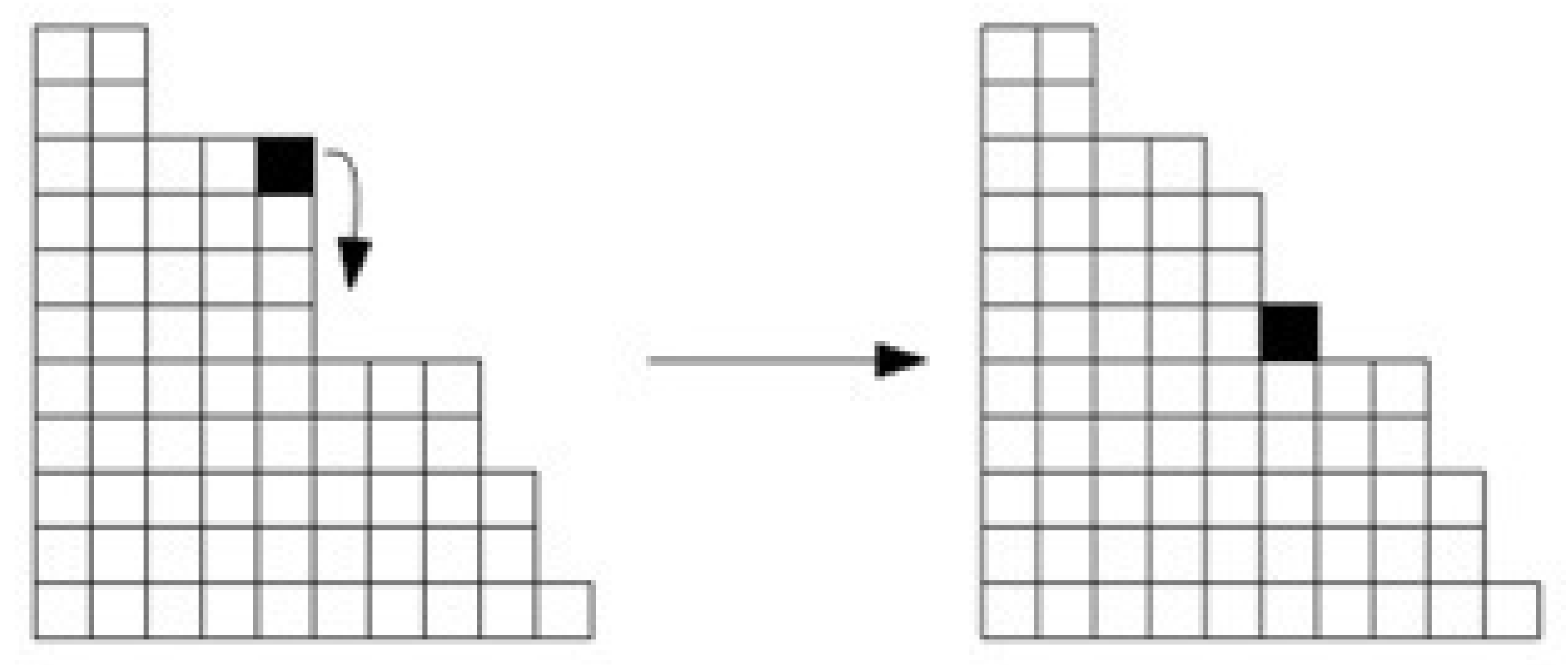
Figure 2.
A schematic diagram illustrating the falling trajectory of a sand grain influenced by wind. Source: [38].
Figure 2.
A schematic diagram illustrating the falling trajectory of a sand grain influenced by wind. Source: [38].
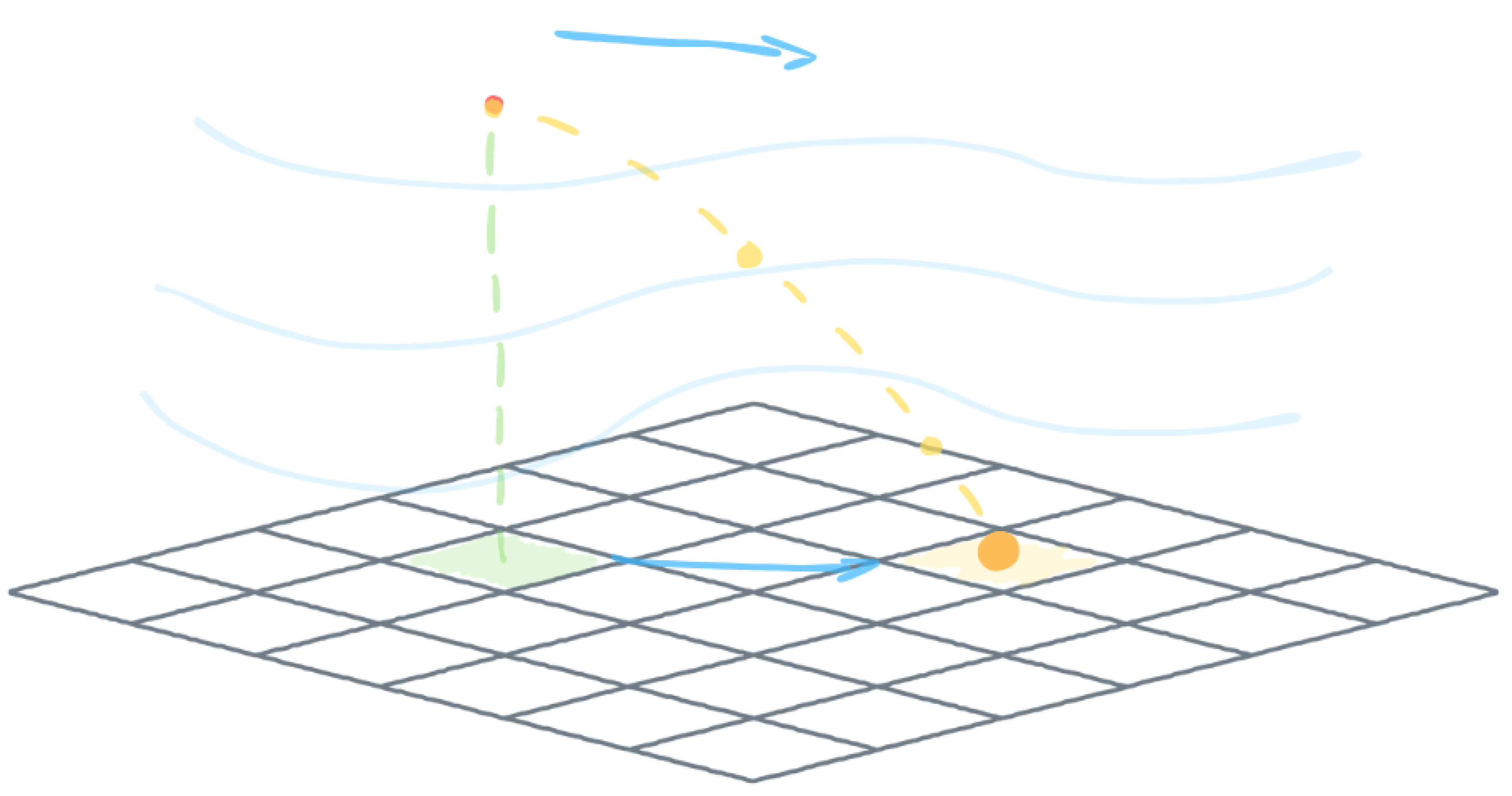
Figure 3.
The source location of the sample release and the spatial distribution of concentrations at ten sensor positions within the sample domain for the Gaussian model.
Figure 3.
The source location of the sample release and the spatial distribution of concentrations at ten sensor positions within the sample domain for the Gaussian model.
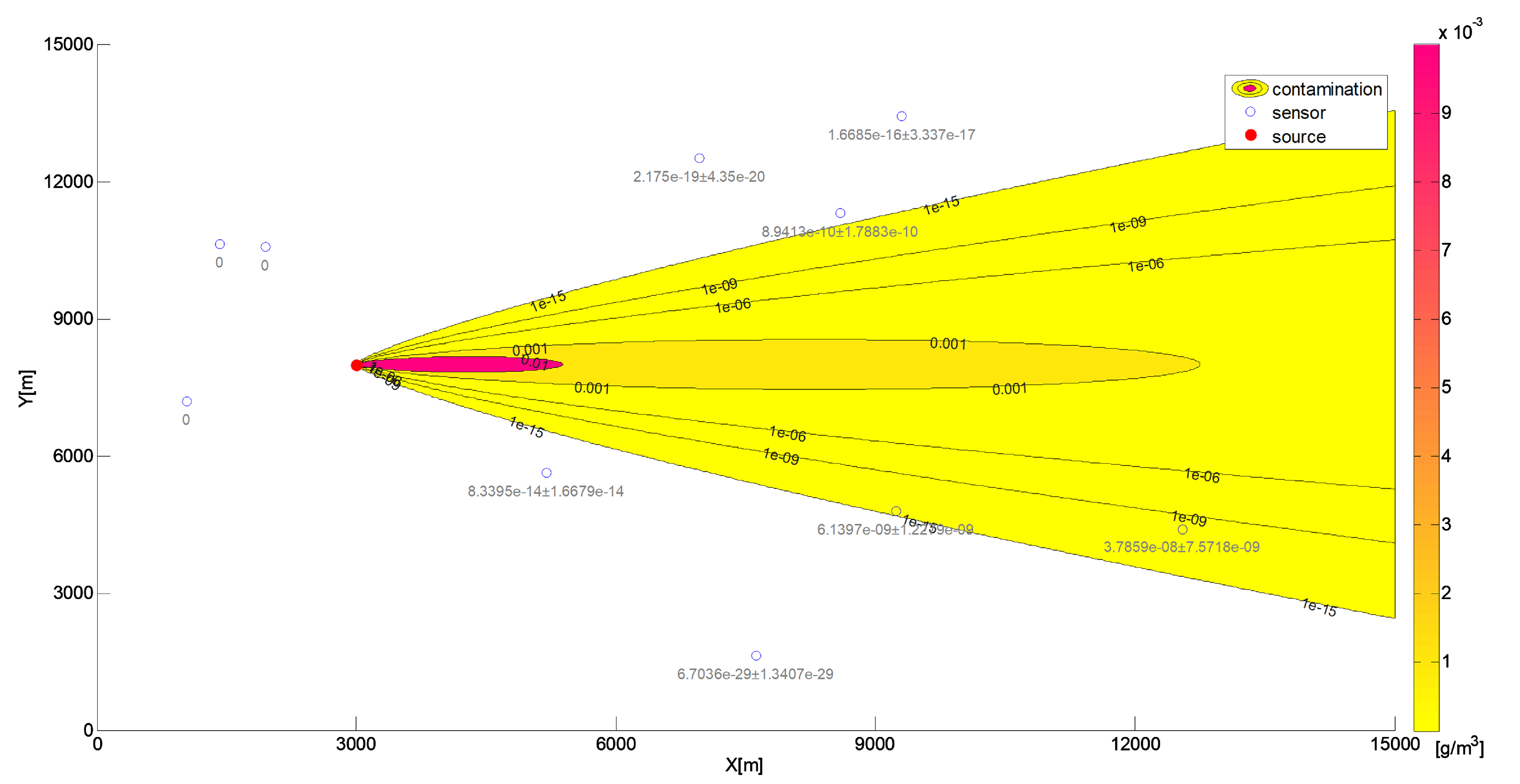
Figure 4.
Heat maps illustrating (left) the typical distribution of 1000 sand grains in the Sandpile model with advection and (right) the contaminant concentration field obtained from the Gaussian dispersion model with an emission rate of . In both cases, the setup assumes a wind speed of directed along the x-axis and a source located at .
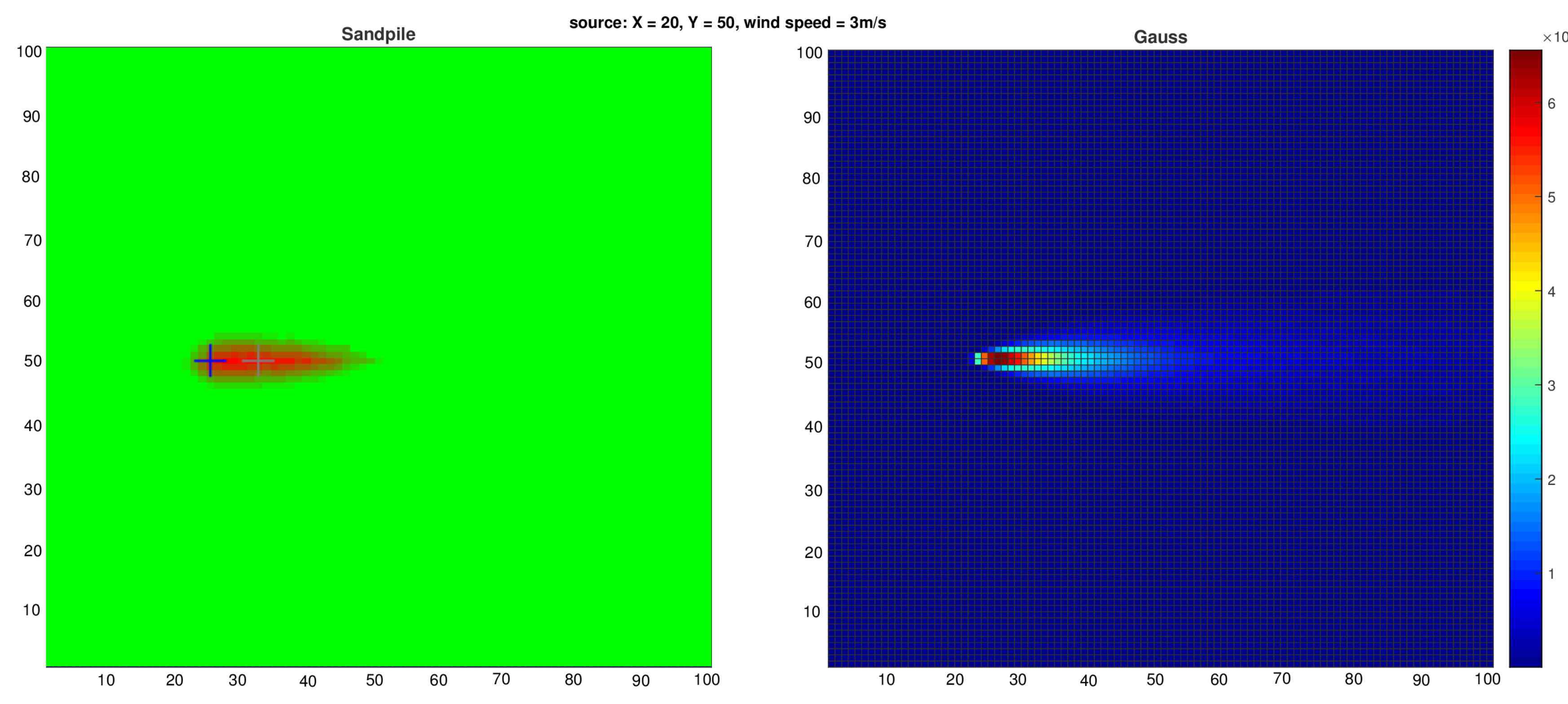
Figure 5.
Three-dimensional distribution of the contaminant concentration for the first testing set with the following parameters: source position , emission rate of , and wind directed along the x-axis.
Figure 5.
Three-dimensional distribution of the contaminant concentration for the first testing set with the following parameters: source position , emission rate of , and wind directed along the x-axis.
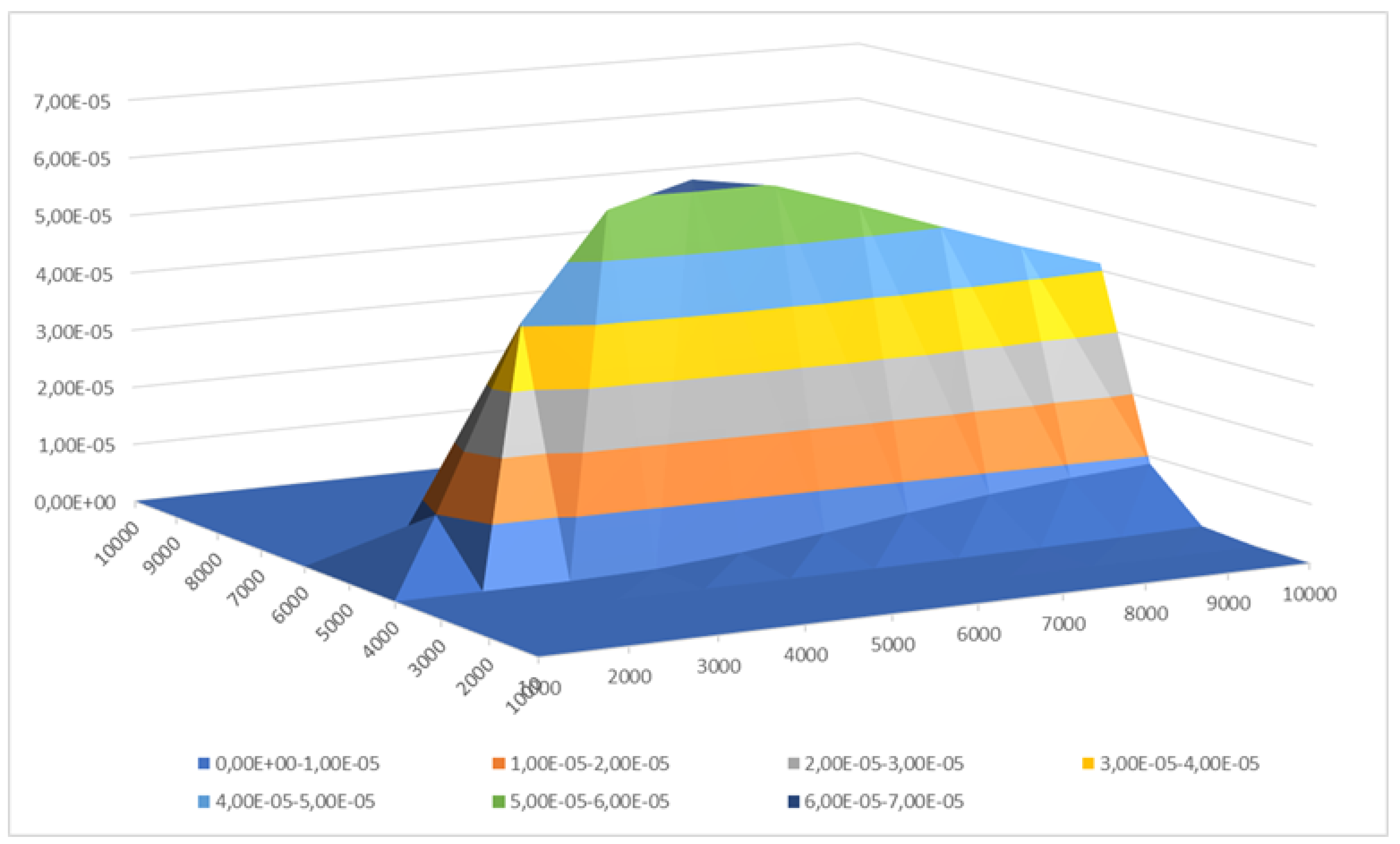
Figure 6.
Contaminant distributions for five datasets used to evaluate the (1+1)-ES Sandpile algorithm in the context of contaminant source identification. Each subfigure (a–e) represents a different scenario modelled with a Gaussian distribution centered at the true source coordinates (in meters) : a) , b) , c) , d) and e) .
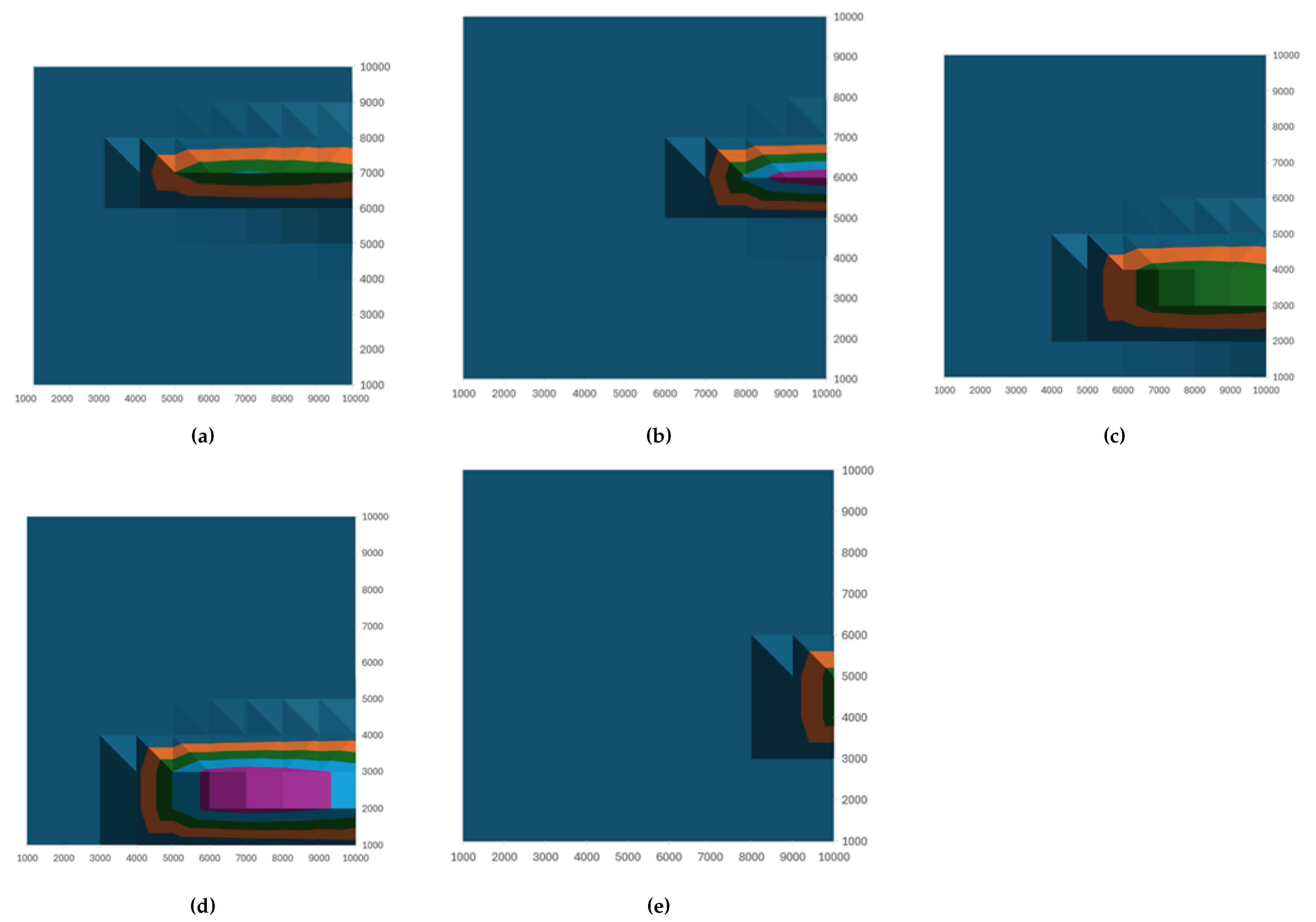

Table 1.
Summary of the optimal configurations for the grain number and grain size , as determined by the (1+1)-ES Sandpile algorithm. The results were obtained under the following constants: , , , and a total of 200 generations.
Table 1.
Summary of the optimal configurations for the grain number and grain size , as determined by the (1+1)-ES Sandpile algorithm. The results were obtained under the following constants: , , , and a total of 200 generations.
| Lp. | X | Y | Z | ||||
|---|---|---|---|---|---|---|---|
| 1 | 0 | 50 | 28.76 | 1,0 | 0.21 | 99540 | 2727.47 |
| 2 | 0 | 50 | 28.76 | 1,0 | 0.19 | 96956 | 2727.52 |
| 3 | 0 | 50 | 28.76 | 1,0 | 0.05 | 77044 | 2737.96 |
| 4 | 0 | 50 | 28.76 | 1,0 | 0.01 | 72947 | 2763.87 |
| 5 | 0 | 50 | 28.76 | 1,0 | 0.05 | 67179 | 2825.11 |
| 6 | 0 | 50 | 28.76 | 1,0 | 0.06 | 50064 | 2903.14 |
| 7 | 0 | 50 | 28.76 | 1,0 | 0.24 | 42460 | 2978.77 |
| 8 | 0 | 50 | 28.76 | 1,0 | 0.28 | 22985 | 3093.93 |
| 9 | 0 | 50 | 28.76 | 1,0 | 0.01 | 11976 | 3106.10 |
| 10 | 0 | 50 | 28.76 | 1,0 | 16.72 | 517 | 3325.24 |
Table 2.
Comparison of the true release source coordinates within the domain for the testing datasets, along with the corresponding source coordinates estimated by the Sandpile model and the (1+1)-ES algorithm.
Table 2.
Comparison of the true release source coordinates within the domain for the testing datasets, along with the corresponding source coordinates estimated by the Sandpile model and the (1+1)-ES algorithm.
| Lp | True source coordinates | Source coordinates indicated by the (1+1)-ES Sandpile algorithm |
||||
|---|---|---|---|---|---|---|
| X | Y | Z | ||||
| 1 | 2946 | 6824 | 29 | 3000 | 6900 | 365 |
| 2 | 5744 | 6075 | 12 | 5800 | 5900 | 201 |
| 3 | 3407 | 4119 | 25 | 3400 | 3900 | 295 |
| 4 | 2455 | 2324 | 16 | 2900 | 3600 | 507 |
| 5 | 7878 | 4633 | 4 | 7800 | 3700 | 21 |
Table 3.
Absolute errors between true source coordinates and those estimated by the (1+1)-ES Sandpile algorithm.
Table 3.
Absolute errors between true source coordinates and those estimated by the (1+1)-ES Sandpile algorithm.
| Lp | True Coordinates | Absolute Errors | ||||
|---|---|---|---|---|---|---|
| X | Y | Z | ||||
| 1 | 2946 | 6824 | 29 | 54 | 76 | 336 |
| 2 | 5744 | 6075 | 12 | 56 | 175 | 189 |
| 3 | 3407 | 4119 | 25 | 7 | 219 | 270 |
| 4 | 2455 | 2324 | 16 | 445 | 1276 | 491 |
| 5 | 7878 | 4633 | 4 | 78 | 933 | 17 |
Disclaimer/Publisher’s Note: The statements, opinions and data contained in all publications are solely those of the individual author(s) and contributor(s) and not of MDPI and/or the editor(s). MDPI and/or the editor(s) disclaim responsibility for any injury to people or property resulting from any ideas, methods, instructions or products referred to in the content. |
© 2025 by the authors. Licensee MDPI, Basel, Switzerland. This article is an open access article distributed under the terms and conditions of the Creative Commons Attribution (CC BY) license (http://creativecommons.org/licenses/by/4.0/).
Copyright: This open access article is published under a Creative Commons CC BY 4.0 license, which permit the free download, distribution, and reuse, provided that the author and preprint are cited in any reuse.


