Submitted:
22 September 2023
Posted:
25 September 2023
You are already at the latest version
Abstract
In the land use planning framework in the neighbourhood of industrial facilities, the current approach to predicting the consequences of massive toxic gas releases is generally based on Gaussian or integral models. For many years, CFD models have been more and more used in this context, in accordance with the development of High-Performance Computing (HPC). The present paper focuses on harmonizing input data for Atmospheric Transport and Dispersion (AT&D) modelling between the widely used approaches. First, a synthesis of the practice’s harmonization for atmospheric dispersion modelling within the framework of risk assessment is presented. Then, these practices are applied to a large-scale INERIS ammonia experimental release. For illustration purposes, the impact of the proposed harmonization will be evaluated using different approaches: the SLAB model, the FDS model and the Code_Saturne model. The two main focuses of this paper are the adaptation of the source term dealing with a massive release and the wind flow modelling performance using an experimental signal for CFD models inflow. Finally, comparisons between the modelling and experimental results enable checking the consistency of these approaches and reinforce the importance of the input data harmonization for each AT&D modelling approach.
Keywords:
atmospheric dispersion models
; atmospheric dispersion of pollutants
; toxic release
; regulatory purposes
; emergency response
1. Introduction
1.1. Toxic gas atmospheric dispersion accidents
Several major accidents occurred in the last decades due to the atmospheric release of dangerous substances. While the most known one is probably the Seveso in 1976 accident [1] with a large release of dioxins since its name was given to the European regulation, others like Bhopal in 1984 [2] with a massive release of methyl isocyanate, the massive release of carbon dioxide in Nyos, Cameroun in 1986 [3] or, more recently in 2022, a large ammonia release in Donaldsonville in the USA [4]. The number of such accidents is important and being able to predict consequences is a huge challenge to protect citizens.
Considering a general point of view in terms of citizens' protection against industrial hazards, following the huge explosion that occurred in Toulouse, France, at the AZF factory [5] causing 31 deaths and thousands (~ 2500) of injured people on September 21, 2001, a dedicated regulation was built. Two years after this major industrial accident, a new regulation was introduced on July 30, 2003, which described both prevention and repair of the damage caused by industrial and natural disasters. This regulation was the beginning of a general change of mind for environmental consequences evaluations, then regulations were made considerably tighter and the entire approach towards risk assessment changed [5] in France. The Technological Risk Prevention Plan (“PPRT” in French, standing for Plan de Prévention des Risques Technologiques) is the new legislation tool aiming to protect people by acting on the existing urbanization and by controlling the future land-use planning in the vicinity of the existing Seveso establishments. The identification of potential scenarios is the first stage of the numerous ones required along the process of the PPRT elaboration. For a scenario that is not demonstrated as physically impossible, this analysis is then followed by the prediction of potential consequences of the associated dangerous phenomena. The prediction of the impact area (thermal, overpressure and toxic effects), which is generated by a dangerous phenomenon, is another required stage. The prediction of consequences is always performed using computational tools. Atmospheric dispersion models are then required to predict distances resulting from toxic or flammable product releases.
Several atmospheric modelling techniques are used in the framework of land use planning, based on a large variety of nature and complexity. For an identical accidental toxic or flammable material release in the atmosphere, within the context of a regulatory study, discrepancies could appear in computed distances, meaning major differences in impacted zones. Those variations can be observed either between atmospheric CFD models or with conventional approaches such as Gaussian or shallow layer approach models. There are numerous reasons behind these disparities, stemming from various sources, and they underscore the clear necessity for harmonization. In the paper, the term “harmonization” is employed to describe the process of constructing and employing AT&D models. This harmonization is essential to guarantee that, regardless of the specific model employed within its designated scope, the results remain highly comparable. Among these disparities, three primary categories can be distinguished: those attributed to the model itself, those linked to the input data utilized, and those arising from user choices.
The aim of the harmonization process is threefold:
- To offer direction during model development, ensuring consistent representation of physical phenomena, especially concerning the relationship between atmospheric turbulence and the diffusion coefficient for pollutants.
- To offer guidance on constructing input data for the model, including factors like the atmospheric wind and turbulence profile, the appropriate roughness value, and the specification of the source term within the AT&D model.
- To provide users with guidance that constrains potential individual choices, particularly concerning numerical parameters or mesh settings.
As atmospheric dispersion modelling continues to evolve as a research area over time, it becomes evident that certain decisions must be made. These decisions should be of a generic nature, guided by harmonization principles, rather than being tailored individually for each study.
1.2. Context of AT&D Model uses
As discussed in the previous paragraph, atmospheric toxic or flammable releases can occur on several installations. AT&D Model capabilities should be considered following several points of view to meet the objective of citizen protection.
The most obvious one is the capability to predict the worst-case situation in the land use planning context. In such an application, all potential scenarios identified during the risk analysis should be modelled crossing the potential release situations with the riskiest atmospheric conditions. The typical result of such an application would be the distances reached by the corresponding thresholds on human beings.
A second application of AT&D Model consists in supporting firefighters in emergency situations by providing information on the potential concentration in the release surrounding. This information is then used either for firefighters’ protection choice or to inform the authorities about the required evacuation as during the above-mentioned Donaldsonville where a school should be evacuated. Having some relevant information about cloud behaviour, in quite real-time is, in such a situation highly valuable.
Finally, AT&D Model should be used to provide more detailed information on a specific case after the emergency phase by detailed modelling of the cloud behaviour or with a research point of view to improve capabilities for the two previous fields of use of such models [6].
It is clear that not the same approach can be used for those different situations since the accident details knowledge differs in-between. In emergency situations typically, in most cases, the source term is just an approximation, during land use planning studies, the source term is a theoretical situation and, in post-accident or research studies, hopefully, the source term is better known. The situation is the same for the wind which is known as a different manner for those different situations.
The scope of application of AT&D Model could be defined in the following six items: release/loss of containment scenario (e.g.: line rupture, catastrophic rupture, vessel burst), material: chemical products involved, hazardous substances/materials, environment, geometry (not targets definition but influencing factors on hazardous phenomena), consequence analysis of hazardous effects, the context of use: risk assessment regulatory study, technical support for a situation of emergency, evaluation of the damage on human health and life, environment or infrastructure.
1.3. Objectives of the Study
The main objective of the present paper consists of breaking down the most common practices in AT&D Modelling for the accidental releases of toxic or flammable gas and putting forward what differences can result from this to provide some thinking about the harmonization of practices between models. From the authors' perspective, this subject is very rarely addressed in the scientific literature. This work represents a new approach to thinking about and illustrating data harmonisation for models.
The harmonization process ensures that the mathematical and theoretical representation of physical phenomena remains consistent, regardless of the level of simplification used by the model. Additionally, harmonization implies that the input data used for modelling are sufficiently well-defined to eliminate any need for interpretation during use.
This paper is structured as follows. In Section 2, an overview is provided of the primary practices in AT&D models for an accidental release, ranging from the simplest models to the most advanced ones. This section also presents descriptions of common models and their utilization, with a specific focus on existing harmonization methods and the introduction of new approaches aimed at enhancing harmonization. In Section 3, the focus shifts to the application of AT&D models to a massive release across various model types. The primary objective of this section is to emphasize the significance of harmonizing each aspect when utilizing AT&D models. This section is then not directly focussed on the application of harmonization practices, since those practices are most relevant for prediction cases within the regulation context. Instead, Section 3 illustrates how each parameter can significantly impact the results, underscoring the importance of harmonizing these practices.
2. Main Steps of AT&D Modelling
The atmospheric dispersion computational models currently used are characterized by a large variety of nature and complexity. For the same analysed hazardous phenomena and physical characteristics, discrepancies appeared in computed distances or impacted zones between models. To provide a better understanding of the origin of these discrepancies, it is important to consider the main physical parameters and the way they are introduced into the different types of models, which will be the objective of the next sections of the chapter.
It's evident that the manner the models deal with physical parameters introduced differences before starting the simulation as typically:
- the representation of the velocity and turbulence profile,
- the description of the emission source term,
- the differences in terms of physical phenomena considered in the model.
A diagram showing the main steps of AT&D modelling within the context of risk assessment is presented in Figure 1. This figure shows the most important topic to be considered in a harmonization process, with the three points of view mentioned in section 1.2, the model, left and right on the figure, input data, in green in the centre, and user, who will run the model and make the choices. In the subsequent section of this chapter and in the following chapter, each element depicted in the figure will be comprehensively explained, outlining its potential impact on dispersion outcomes.
2.1. Background about theoretical approaches
A major issue for risk assessments is the harmonization of input data for the atmospheric modelling between widely used approaches, from simple gaussian or integral model to more complex one as CFD (RANS or LES) approaches which using is continuously increasing due to easier use to High Performance Computing. To the best of the authors' knowledge, other approaches exist but are not yet widely used [6,7] at the microscale scale.
2.1.1. Gaussian models
The simplest and probably the most used approaches are Gaussian models. Such models are rigorously restricted to neutral gas dispersion for releases that do not affect the atmospheric flow, such as low momentum releases, this means that the released gas should have a density close to the air one or have been diluted enough. Such an approach assumes that atmospheric turbulence is the key parameter for gas dispersion that enables assuming a Gaussian-distributed gas concentration following the orthogonal directions of the flow [8]. Characteristics of atmospheric turbulence are then introduced through the standard deviation coefficients, s, in the concentration equation. Among these, two main Gaussian approaches could be distinguished, the first series is designed for free field dispersion the second one includes analytical corrections to take into account obstacles [9]. A typical equation of the gas concentration, C, in space (x,y,z) and time, t, evolution can be written, for a local and instantaneous release, as follows:

with M the discharge product (kg), u the mean wind speed (m/s), t time since the emission of the product, (x0, y0, z0) the discharge location, α a reflection coefficient on the ground. The standard deviation coefficients σx, σy, σz of the Gaussian distribution of the quantity of gas M in relation to its position at the instant t [m], are then based on experimental data and several available sets in the literature are those proposed by [10,11,12].
2.1.2. Integral models
When the discharge is such that it disturbs the atmospheric flow of air, it is inappropriate to use a Gaussian model, at least in the vicinity of this release. Physical mechanisms not considered by Gaussian models must be considered, such as the effects of dynamic turbulence. These concerns typically discharge with a high emission velocity such as a jet; the effects of gravity for heavy gas discharges; the floating effects for light gas discharges. The use of an integral model allows these mechanisms to be represented and it explains the wide use within. This type of model is based on simplified fluid mechanics equations set to provide a quick solution. The scalar conservation is assured by the integration into the volume delimited by the surface of the cloud, from whence comes the “integral approach”. In addition, these models include, in most cases, a calculation module enabling the discharge source term to be determined according to the product’s storage conditions and the type of discharge (full bore-rupture tank rupture, pool evaporation, etc.) [13]. As soon as the release becomes passive, i.e. diluted enough and low enough velocity, integral tools transition to a Gaussian model.
2.1.3. Shallow layer models
A specific family of integral-like models was developed to deal with heavier than air gas dispersion. Such models are based on one-dimensional equations of momentum, conservation of mass, species, and energy, and the equation of state resolution. It can handle release scenarios, instantaneous, continuous or with a finite duration, including ground level and horizontal or vertical elevated jets, liquid pool evaporation, and instantaneous volume sources for the specific case of heavier than air gases since this enables simplifying the equation set resolution. One of the most known shallow layer models is SLAB [14].
2.1.4. CFD modelling
CFD (Computational Fluid Dynamics) approaches consist of solving the full set of Navier-Stokes equations after having discretized the computational domains in cells. During a dispersion process, the key physical phenomenon that governs the gas mixture is turbulence. Solving the turbulence is the heart of those CFD models, and two main approaches can be used in that way, RANS (Reynolds Average Navier Stokes) [15] or LES (Large Eddy Simulation) [16] approaches for industrial application, DNS (Direct Numerical Simulation) is not realistic for such a large domain. One of the main differences between RANS and LES, is the isotropic hypothesis for the turbulence used in most of the RANS approaches while, in LES models, only the modelled small scales are assumed as isotropic, the solved scales, the higher ones, are not, meaning that the turbulence anisotropy could be solved [18,19]. Having in mind that atmospheric turbulence is strongly anisotropic, this is of primary importance. Another way to keep the anisotropic properties in the model is to use Rij models [20].
Obviously, choosing the turbulent model implies considering the main physical parameters to be considered in it. An important aspect of atmospheric turbulence is the important relation between the thermal gradient and the turbulence that leads to the distinction between:
- the neutral atmosphere, where the thermal gradient corresponds to the adiabatic gradient;
- the stable atmosphere, where the gradient is lower than the adiabatic one;
- the unstable atmosphere, where the gradient is higher than the adiabatic one.
Such a gradient would induce some convective displacement and of course influence the turbulence, which means that the thermal gradient influence should be considered in the turbulence model. Once more, natively in the LES approach, the turbulence anisotropy [23] and the density effect on the turbulence are included in the equations since they affect more specifically larger scales. On the opposite, in the RANS approach, an additional term should be added to the transport equation to introduce the density gradient influence on the turbulence. For such a specific application of k-e models, [21] proposed a specific set of constants together with an additional term in the k equation:
where b expresses the floatability, b=g/qv, is the fluctuation of the potential temperature and w’ the fluctuation of the vertical velocity component.
An important constrain of the LES approach however is the mesh criteria, based on the fundamental principle of the LES approach, the resolved part of the turbulent should be important enough [19] with a minimum criterion that consists of a characteristic cutting scale in the inertial zone of the turbulent spectrum [22]. Since the same turbulent intensity can correspond to different turbulent spectrums, producing a reference method to build a representation of atmospheric turbulence from an LES point of view would be a great improvement.
Based on this state of the art, some recommendations should be proposed towards harmonization of CFD practices including:
- the turbulence model should consider the influence of the thermal gradient on the turbulence generation of suppression;
- the atmospheric turbulence anisotropy should be considered as a target when developing atmospheric dispersion models;
- developing of LES harmonized practices to build the input turbulence.
2.1.5. Harmonization between model input data
The objective of harmonization between AT&Model is to achieve input data for each model considering their respective domains of use. Some simplifications describing ABL, particularly in the regulatory context, are sometimes necessary such as the stationary nature of ABL over the modelling period. Indeed, as defined by Stull [25] the atmospheric boundary layer is the part of the troposphere directly influenced by the presence of the Earth's surface such as it responds to surface forcing on time scales of the order of an hour. Starting from a hypothesis of stationary it is necessary to make a choice on the vertical speed gradient and the vertical temperature gradient. These gradients are mainly due to the effects of air friction on the ground and heat exchanges between the ground and the atmosphere. These exchanges vary with the diurnal cycle, weather conditions and the nature of the soil. At the end, a harmonization of meteorological data pre-process means focusing on fundamental values describing ABL, such as Monin-Obukhov Lenght (LMO), friction velocity u*, wind speed (m/s) at an altitude reference, the roughness, and the turbulent sensible heat flux. Meteorological profiles construction will be given in detail in the next section.
2.2. From meteorological conditions to AT&Model flow input data
Depending on the context, the nature and completeness of the flow data are fundamentally different. Mean wind at a reference altitude and information about the atmospheric turbulence stability seems the minimal set of data to characterize the flow. A frequently used characterization of atmospheric turbulence stability is the turbulence classification scheme originally developed by Pasquill [12]. It categorized the atmospheric turbulence into six stability classes named A, B, C, D, E and F with class A corresponding to the extremely unstable cases, and class F to the moderately stable cases. In the context of an emergency, directly observed data by first responders or extraction for meteorological corrected forecast [26] can be scarce. Measured mean wind at a reference altitude and observation in situ, such as daytime insolation or cloudiness during the night, may be sometimes the only valid data available. Then, from [24] it is possible to diagnose a Pasquill turbulence type. For the simpler models such as Gaussian, shallow layer or integral, these Pasquill classes very often constitute a direct input.
However, while this should appear implicit for Gaussian or integral models where wind profiles and standard deviations are given for the whole dispersion zone, in real cases, this is not so obvious. To address this topic, one should consider how these models are built, generally based on experimental observations in a free field zone, with a certain ground roughness as mentioned above in this paper. Then, when considering a real accident that leads to dangerous substance release into the atmosphere, wind and turbulence profiles cannot be constant, these profiles would be modified by buildings, and mainly industrial installations, where the leak originates. An important consequence of this intrinsic hypothesis of the model is that the industrial facilities induced turbulence that is not considered. Having in mind that turbulence is the main physical parameter that governs dispersion, it appears clearly that those models would tend to overestimate distances. Indeed, using variable standard deviation coefficients would require one to evaluate them, which is not so far from the objective of the CFD models since this corresponds to an evaluation of the diffusion coefficient in each zone of the domain. The same limit can be mentioned for integral models since they generally transition to Gaussian dispersion for the passive cloud dispersion. On top of the standard deviation coefficients, most of the Gaussian models also consider a constant ground roughness, such as roughness is also an important parameter for the wind profile and for the dispersion calculation.
In an item from the French circular of 10 May 2010 (sheet 2 and sheet 5), recommendations are given on the choice of meteorological conditions in the context of hazard studies (French regulation). The atmospheric stability conditions generally used for ground-level releases are type D (neutral) and F (highly stable) as defined by Pasquill. These are associated with wind speeds of 5 and 3 m/s respectively. Those conditions were defined to represent the worst-case conditions for land use planning studies. In the end, the Pasquil class and a wind velocity are associated to a roughness value to form the set data for swift model.
Harmonization of input data for flow and boundary layer simulation between the swift models and more sophisticated ones remains a major issue within the context of regulatory studies. For an atmospheric condition defined only with three parameters (Pasquill class, velocity module at reference height, and ground roughness) several profiles are then possible. Gaussian models are commonly using highly simplified mean velocity profiles, 3D models need more sophisticated profiles for different physical quantities such as wind, temperature and turbulence profiles. It is also obvious that, in most industrial cases, not only the surface boundary layer must be modelled but the entire atmospheric boundary layer. For regulatory reasons and consistency with existing computation, it is important to limit the set of input parameters for meteorological data as much as possible.
A roughness length is also required to characterize the environment of the industrial plants. It is obvious that such conditions cannot be translated easily to a 3D model approach.
Having in mind that velocity and turbulent inlet profile is one of the key parameters, the homogenization of the inflow boundary conditions is still an open issue. The relation between Pasquill classes and tridimensional inflow boundary conditions is difficult to establish because the classes of Pasquill represent a broad variety of possible states of the atmosphere, as illustrated by the well-known diagram of Golder [24]). Few approaches have been proposed to make the link between atmospheric flow input data, such as Pasquill class and input data for CFD models. However, it can be mentioned some approaches intended for RANS approach ([27,28]), briefly described as below
In the French guide for atmospheric dispersion modelling [27], a specific method was proposed, mainly for RANS simulations. This method consists in representing the wind profile thanks to the Gryning description [29] that links the velocity profile to the Monin Obukhov length for extending profiles beyond the surface boundary layer. There is, unfortunately, no bijection between Pasquill stability classes and the Monin Obukhov length and a user choice is required [30] for a given roughness, especially for classes A and F. This leads to an iterative calculation to estimate the friction velocity near the ground, u*0 that matches with required wind module at height reference. The hypothesis of local friction velocity [25] was considered consistently with wind profile formulation. Knowing the velocity profile, it is then possible to build the kinetic turbulent energy and dissipation profiles, based on the equilibrium hypothesis [31]. Having built the turbulent profile, turbulent characteristics are known, especially the typical turbulent length scales that made it possible to build the required data for LES profiles. Obviously for experimental comparison when all these parameters are available, the data pre-processing needs less complexity.
Even though wind and turbulence profiles are used as input profiles for CFD codes, they may be modified along a flat, unobstructed domain when the equilibrium state is reached by the code. Indeed, a previous study has demonstrated [32] the difficulties for RANS CFD models to maintain the ABL profiles along a domain longer than ~1000 m [32]. In addition to the difficulties associated with the wall functions model [33], the difficulty of performing an inlet profile consistent with the turbulence model is still an issue open issue when users have to demonstrate the capability of the RANS CFD code to maintain a steady wind and turbulence profile along a flat, unobstructed domain. This demonstration is considered as a requirement by practice guidelines [27]. This unresolved problem for RANS and LES CFD code should drive research.
2.3. From toxic emission assessment to term source implementation
At an industrial scale, substances (raw materials, finished products) can be stored in tanks, spheres, bottles, containers, barrels, etc. They can be stored as compressed gases or as liquid, refrigerated or not or of a liquefied gas. For the last two cases, any accidental release of these products will lead to a two-phase emission that can induce the formation of a pool. Then, the resulting cloud is heavier than air due to aerosols and evaporation phenomena. The assessment of toxic industrial chemical (TIC) emission rates is still a major issue as put forward by Britter [35]. Whereas the implementation of the source term for a Gaussian model can be summarized as a gas flow rate, the added value of a sophisticated source term for CFD models is an issue. Firstly, a massive release generated a lot of complexity to handle phenomena in the near field [21], secondly, a simplification of the setup in a sophisticated model is sometimes desirable to avoid too much study time consuming, particularly in the context of emergency management. Indeed, although work has been continuously done on two-phase discharges jet, for two decades ([36,37,38]), this is still costly in terms of calculation time.
Considering all these factors, it is advisable to employ a simplified source term. Therefore, the use of an equivalent source term [39] at a certain distance from the orifice to bypass limitations mentioned above, thus leading to moderate velocity and a weak liquid fraction which can be readily handled by CFD code is relevant. Such an approach is typically schemed in Figure 2 for massive release studied in Section 3.
The use of a simple approach such as a 1-D or 2-D model to ensure the conservation of parameters from orifice to inlet boundary area is strongly recommended [39].
3. Application to an experimental case
To illustrate the theoretical description made in the previous paragraph and the harmonization requirements, an application to an experimental case is carried out, highlighting the significant stages that were identified before: implementation of source term emission, choice of calculation domain, mesh generation, boundary conditions, choice of physical sub-model. The source term modelling is one of the most important steps. The massive release test case is presented in the next section. This case was targeted because it was deemed as a toxic massive release representative of an unobstructed environment, which is within the application domain of all AT&D model types. Through this result presentation, a special focus is made and the potential improvement of harmonization.
3.1. Description of the experimental dataset
Ammonia dispersion field tests performed by INERIS were presented in a previous paper [40]. INERIS conducted real-scale releases of ammonia on the 950-ha flat testing site of CEA-CESTA. Figure 3 shows the whole measurement area.
During experiments, the atmospheric conditions were analysed using a 10 m height meteorological mast equipped with 3 cup anemometers located at 1.5, 4 and 7 m above the ground, a wind vane at 7 m and an ultrasonic anemometer at 10 m. A weather station was also installed in the vicinity of the testing site. It allowed recording the ambient temperature, the relative humidity, and the solar flux 1.5 m above the ground. Sensors were located in 7 arc shapes centred on the release point. Several release test cases were achieved with a mass flow rate up to 4.2 kg/s and a two-phase release. For the scope of the present paper, case 4 is considered, it corresponds to a free field horizontal 10 min long release. The mean wind direction is indicated in Figure 3 thanks to the blue line. In this study, an enhanced wind flow analysis is carried out to take into account additional measurements provided by an ultrasonic anemometer (see Table 1).
3.2. Atmospheric dispersion modelling by “swift” model
The widely used dense gas dispersion SLAB has been used to simulate the trial case. It is available for free thanks to the Environmental Protection Agency (EPA). The model can handle horizontal jets [41]; in the far field a shallow-layer approach is widely used to disperse a dense gas according to the observed behaviour of the release. This model is well suited for emergency situations; indeed, it allows us to obtain a swift estimation of effects distances and it has been used in many comparisons with heavy dispersion gas dispersion campaigns at large scale [41,42]. The model was run in diagnostic mode with the optimum source release terms knowing the experimental mass flow rate and that experimental observations showed very little rainout deposition on the ground. The flow input is set by the stability Pasquill (see Table 1), according to the sonic anemometer measurements, and a roughness value of z0 = 0.03 m was selected according to the land cover of the experimental site ground (prairie grass).
3.3. Adaptation of the experimental atmospheric signal for CFD model inflow
3.3.1. Turbulent closure and inlet boundary conditions
The RANS CFD simulations were performed using Code_Saturne, which is a general-purpose open source CFD code (www.code-saturne.org) [43]. It has been previously tested on flat terrain [44] and obstructed environment [45]. The governing equations are solved under Boussinesq's hypothesis. Simulations were run with an atmospheric flow adapted k – ε turbulence model [47]. The transport equations for the turbulent kinetic energy k and the scalar dissipation rate, e, consider the wind shear and buoyance effect on the production or dissipation of k. This latter term is formulated by means of potential temperature gradient. Indeed, the transport equation for the potential temperature, q, profile is solved along the domain. The models constants for k – ε turbulence model are those modified for atmospheric flows following [48] where Cµ = 0.03 according to the work of Duynkerke [48] and the value of Cε3 is taken after [49]: Cε3 = 0 for a stably stratified atmosphere and Cε3 =1 for an unstably stratified atmosphere corresponding to the present studied case.
The atmospheric stability class is represented by the inflow boundary condition for the velocity, the turbulent kinetic energy k, dissipation of turbulent kinetic energy ε and temperature profile. The inlet and the top boundary are specified by the Dirichlet condition. The outlet is a free outflow condition. The lateral boundaries are symmetry condition. In previous computational fluid dynamics (CFD) flow simulations [45], it was observed that improved outcomes could be achieved by adjusting the inlet conditions to match measurements for both the mean velocity profile and turbulence intensity. Hence, the formulation for the wind and turbulence profile was selected to achieve a more satisfactory comparison between the CFD inlet conditions and the experimental profile (see Figure 4). A power law velocity, according to the stability class reported by Barrat [46], i.e., n = 0.16 (stability class C). The scalar dissipation rate profile is based on the hypothesis that viscous dissipation balances shear production and buoyancy. The inlet profiles of k, ε and the turbulent viscosity, Km are specified as follows [31]:
The LES CFD simulations were achieved using FDS a freely available CFD code provided by the NIST [50] and initially dedicated to gradient density-based flow modelling. As discussed previously in this paper, the focus for LES is not inside the domain since the main effect of the flow on turbulence is explicitly solved but is for inlet boundary condition. When using LES, defining a representative turbulent flow field as an inflow boundary condition is an issue. The flow should satisfy prescribed spatial correlations and turbulence characteristics as required by the well-known synthetic eddy method (SEM) [51]. The method used in the present study is based on physical assumptions, it consists in generating a synthetic turbulent velocity signal written as a sum over a finite number of eddies with random intensities and positions. It is based on the observation that large-scale coherent structures in turbulent flows carry most of the Reynolds stresses. More precisely, the method involves the generation and superposition of a large number of random eddies (N), with some control on their statistical properties and using the following predefined shape function for the velocity fluctuation (see equation (3) in [51]). These eddies are then transported through an 800 m long rectangular cross-section domain. The resultant, time-dependent, flow field taken from a cross-section of this domain can be extracted and imposed as an inlet condition for LES. This method allows the desired Reynolds stress field to be prescribed. Inflow boundaries for synthetic method available in FDS consists of data given by following experimental results: mean velocity (Umean), Root Mean Square velocity in x-direction matching with mean wind direction (RMSx), Integral time scale (Tx), integral scale in x-direction (Lx). The inflow mean velocity profile follows an exponential law. Integral length scale may be defined by assuming the advection of turbulent structures by the averaged wind such as: Lx = Umean x Tx with Tx the observed integral time scale in x-direction. The atmospheric data used as inflow boundary conditions for LES approach are presented in Table 2. The number of eddies is equal to 1000.
RMS velocity fluctuation set up at inlet is isotropic. In other words, diagonal components of the Reynolds stress are identical, and all others are set to 0. The outlet is a free outflow condition. The lateral boundaries are symmetry condition. No temperature profile is set up at the inlet.
3.3.2. Mesh and numerical set-up
The physical domain used is 1300 m x 600 m x 60 m in the x, y and z directions, for RANS and 800 m x 400 m x 40 m for LES. The computational grid consists of approximately 1.2 million of hexahedral volume elements for RANS (expanded grid with an expansion ratio lower than 1.2) and 2 million hexahedral volume elements for LES. The minimal space length is 0.5 m corresponding to cells located close to the ground, it allows implementing the source term with 4 cells (see Table 3).
3.3.3. Wind and turbulence profile advection
The first step in the whole simulation task consists in checking whether the wind flow is correctly modelled or not to demonstrate that a homogeneous ABL is obtained along the whole domain. For the RANS approach, the results show that the ABL profiles are well sustained, except for the turbulence kinetic energy which decreases downwind the inlet. Difficulties faced in the present atmospheric condition (slightly unstable) were expected and this issue is addressed by previous works [32,55]. However, it turns out that turbulent viscosity profile (see Figure 1) is eventually quite well sustained along the domain close to the ground (z < 5 m). Consequently, it is assumed that the difference between ABL profiles at inlet and at outlet generates a weak impact on dispersion predictions. Moreover, the theoretical profile used to build the input turbulence slightly overestimates the value measured by sonic anemometer at 10 m height (see Figure 4) such the level of turbulence modelled by Code_Saturne could be deemed close to the one observed during the test.
Figure 5 shows the flow characteristics obtained with LES approach at different x-positions and compared against inflow conditions and experimental data.
Mean velocity is well maintained in the domain. However, turbulence decreases rapidly in the first part of the calculation domain, but RMS profiles are sustained in a steady way. This turbulence decrease was expected [52] and explained the underestimation of friction velocity when compared to experimental data. Other strategies exist to set up a LES [56] modelling, but to the best of the authors' knowledge, few studies have been carried out on an industrial site scale. These clear highlights that, while LES offers a theoretically relevant approach for atmospheric dispersion since it enables natively considers the flow properties, the practical use is more complex and challenging due to the large domain to be modelled and the interaction of the flow with the ground to get equilibrate turbulent profile.
3.4. Implementation of a Biphasic Dense Gas Source Term
FDS and Code_Saturne cannot directly deal with high-speed multi-phase releases. Then, an equivalent source term (see Table 3) was implemented at a distance from orifice to bypass this limitation, thus leading to moderate velocity and a weak liquid fraction which can be readily handled by CFD code. Knowing the ammonia experimental mass flow rate, the general properties of the fluid in the very near field are obtained by means of a weighting operation between the gas and the liquid near the orifice within the Homogeneous Model (HEM) [35]. This latter is combined with Papadourakis et al. [57] approach to simulate a biphasic jet to compute a source term and set up a gaseous source term equivalent. It is then implemented as a monophasic equivalent term source in FDS and Code_Saturne simulation. A summary of this latter is given in Table 3.
3.5. Synthesis of model inputs
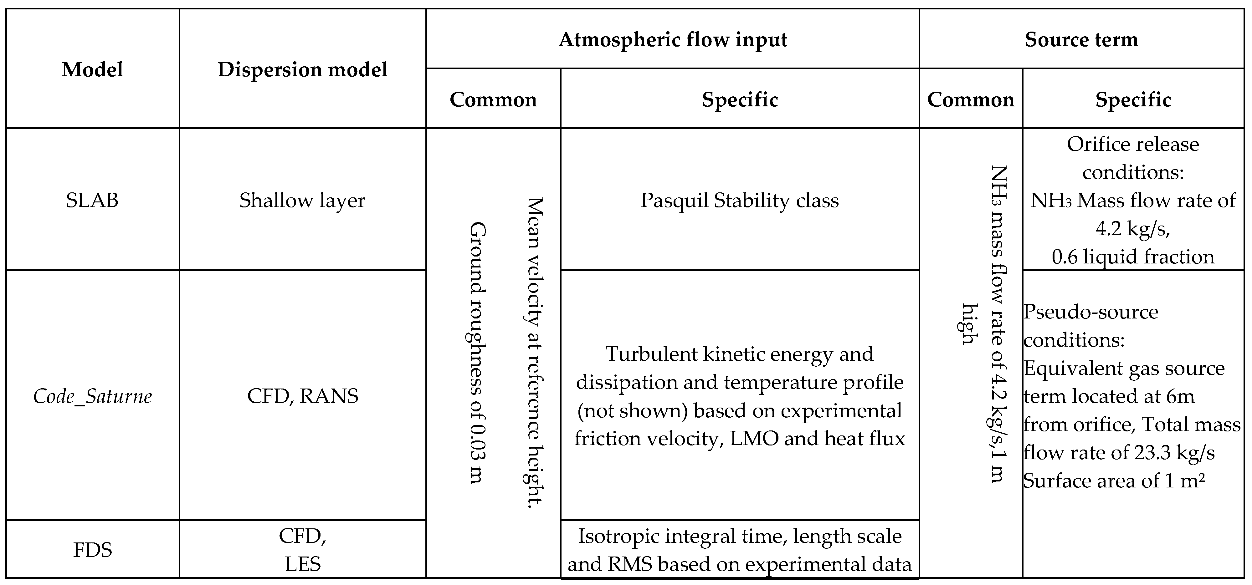
Table 4 summarizes the data used as inflow boundary condition and for emission source term for the three approaches used in this study. This table points out the common input that are used and the discrepancies that appear before running the simulation itself, just due to setting the calculation.
3.6. Comparison of measured concentrations with Atmospheric Dispersion Modelling results
One of the key results provided by AT& D is the concentration profile along the wind axe. Indeed, it allows obtaining a swift estimation of safety distance by cross-referencing the toxic concentration threshold. Comparison between simulation results obtained with the three models and experimental concentration data at z=1m along the main wind axis is presented in Figure 6. The set of experimental observations correspond to maxima of mean conditional concentration values (red square in Figure 6, in Figure 7 and in Figure 9) observed by sensors for each arc. According to definition of previous studies [49,50], these concentrations are determined from the mean of non-zero concentrations during the lifetime of the signal. The sensors involved for trial 4 are located on 23, 25 and 25 axes (see Figure 3). The corresponding concentration for CFD model (at z=1m) are presented for a rigorous comparison. The averaging time roughly corresponds to the exposition time period defined by arrival time and departure time of the cloud. SLAB results correspond to concentrations, obtained with an averaging time of 600 s, at a heigh where maxima are obtained (in this case at 0 m < z < 1 m) along the wind axe.
It can be noticed that global tendency is quite well reproduced by all approaches. The concentrations decrease, along the mean wind axis, modelled by SLAB and the observations can be deemed in good accordance, particularly in the near field (x < 200 m). This is to be put in relief with the easy use of this kind of model, particularly when it is needed to obtain an order of magnitude in emergency situation. However, in the far field (x >200 m) (see Figure 7), this swift model underestimates the level of concentration illustrated by the threshold of toxicity for 10 min exposure (866 ppm). It results that corresponding distance is roughly underestimated by a factor ~ 1.5.
For RANS and LES approaches these results are promising regarding the complexity to describe both the release in the near field and the far field. However, the model slightly over-predicts the measurements respectively in the near field (50 m < x < 200 m) for the RANS model and in the far-field (x > 200 m) for the LES model. An explanation could be the insufficient level of mixing due to the atmospheric flow. Indeed, previous studies [60,61] demonstrated this possible k- ε and LES turbulence model's weakness.
Visual observations show clearly that the ammonia cloud (see Figure 8 (a)) is dense and moving near the ground far from the source. The amount of initial liquid fraction within the experimental cloud is much larger than critical value, estimated between 4 and 8% of the total mass of ammonia for air at 293 K by previous studies [62], such as the cloud remain denser than the surrounding air regardless of the humidity of the air.
The modelled cloud of ammonia by FDS behaves well as a dense gas around several hundred meters. A roughly comparison between FDS modelling results and experimental observations shows that whole shape of the modelled cloud at 500 ppm is in good accordance with experimental observations, (Figure 8) which indicated the plume is visible until approximately until 500 m [40]. This figure typically shows that the modelling tool is able to reproduce with a quite good agreement the typical shape of the cloud. This level of concentration corresponds to toxic threshold (French Acute Toxicity Threshold Values) for irreversible on human health in case of 30 min exposure. That time exposure can be deemed as a representative exposure time for a lot of unintended toxic release scenarios within an industrial risk assessment context.
According to Carruthers et al. [63] it can be considered that the cloud is visible as soon as the liquid water content (rliq) is greater than 10-5 kg/kg. A very simplistic and roughly estimate can be carried out using the method proposed by theses authors. Starting from an initial mixing ratio value at the release point that is around 220 g of NH3 by kg of air (see Table 3), it appears that for a dilution of 500 ppm the mixing ratio value of the cloud, rcl, is around 43 g of NH3 by kg of air. For an ambient humidity of 82% (trial 4), the saturated mixing ratio, rsat, is around 10 g/kg. It results out that rliq = rcl - rsat is >> 10-5 kg/kg, such as the CFD modelling result combined with a simplistic estimate tends to confirm that the cloud is visible at a level of 500 ppm in the trial 4 ambient conditions. Severe difference in terms of plume visibility would be obtained in case of distinct ambient conditions, this issue is put forwarded by recent research projects [64].
Comparison between CFD model results and observations are presented for each arc concentration sensors in Figure 9.
Figure 9.
Comparison between simulation results (FDS: continuous line; Code_Saturne: dotted line) and experimental concentration for each arc (A=20 m, B=50m, C=100m, D=200m, E=500m, F=800m) of receptors.
Figure 9.
Comparison between simulation results (FDS: continuous line; Code_Saturne: dotted line) and experimental concentration for each arc (A=20 m, B=50m, C=100m, D=200m, E=500m, F=800m) of receptors.
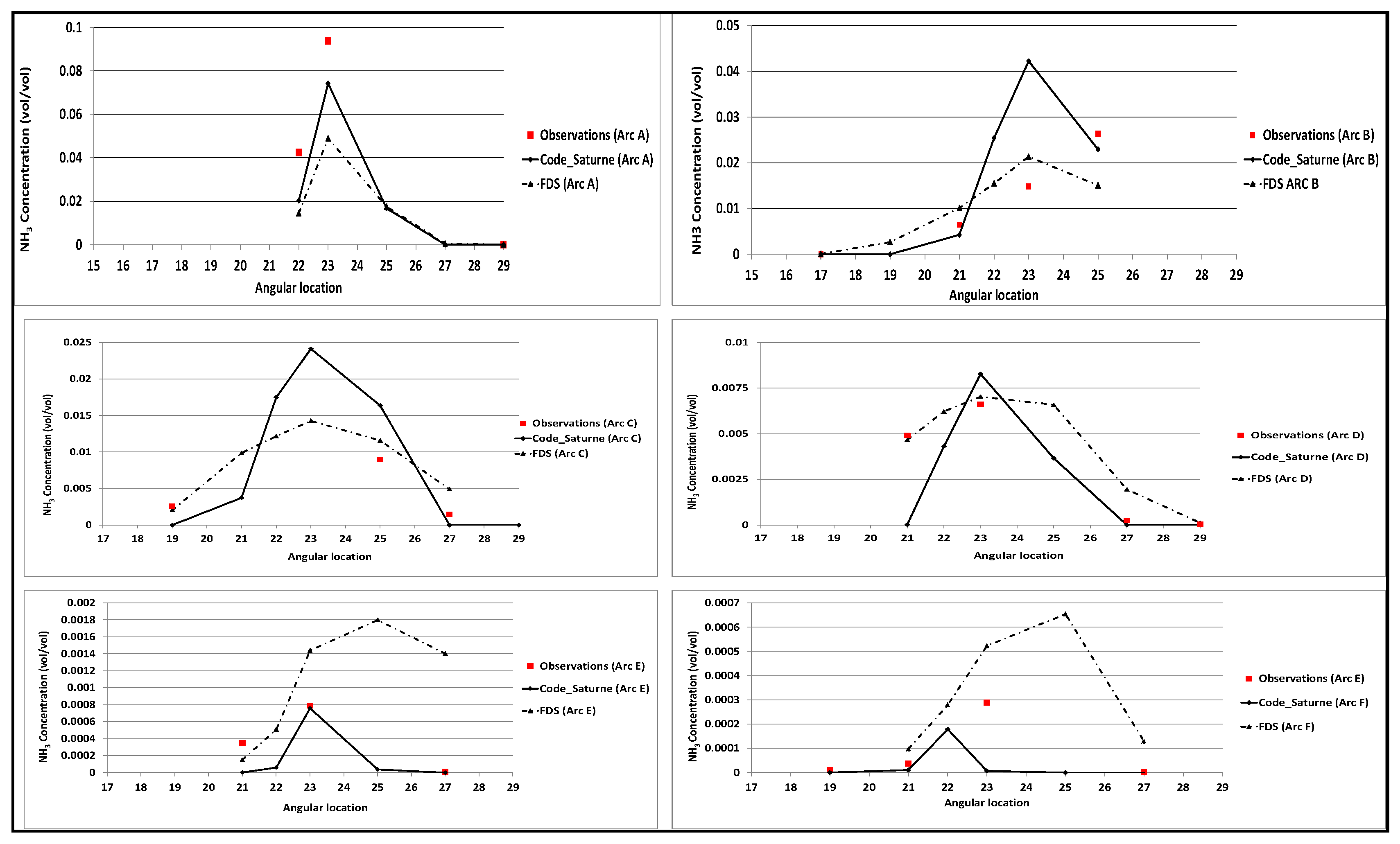
It appears that simulation by FDS overestimates far field concentration while simulation by Code_Saturne underestimates the plume width. This comparison is a good illustration of the difficulty to assess all the phenomena both in the near field and the far field. Bearing in mind the use of an equivalent gas source term, these results are very promising. This study should be considered as an essential stage for validate the use of CFD model in the context of regulatory studies where the need of assess obstructed environment will be of primary importance.
3.7. Outcomes for best practices within regulatory context
Modelling of the experimental massive release has highlighted practices about data processing and sub-model choice and their influence on the results. The main outcomes to bear in mind for regulatory context are synthetised in this sub-chapter.
The turbulence and wind inlet profiles for various stability classes are of such significance that they must be formulated based on consensus-established equations for swift model and CFD codes. Indeed, they directly impact the pollutant atmospheric dispersion by means of turbulence diffusion and advection phenomena. Generating these profiles (see section 3.3.1) is intrinsically related to a unique roughness value, for wind velocity value at heigh reference and friction velocity value. As illustrated in previous section, the two first parameters when combined with Pasquill class are generally a direct input for swift models. Friction velocity value is a sensitive parameter sensitive as it largely influences both turbulence and wind profile. This reinforces the need in regulatory context to propose a common method to estimate its value, starting from the lost simple data set. A single roughness height may characterize the entire area of interest for an accidental release at local scale. An enhanced study, based on a statically wider wind study of the site, would be necessary to assess this value which is generally sensitive for atmospheric dispersion modelling. The choice of inlet profile formulations for RANS CFD should be done consistently with the choice of sub-model turbulence for RANS approach [27, 32] to reach a satisfactory equilibrium state for ABL. For LES CFD approach a more complete turbulence set of data can potentially be assessed as illustrated in table 4. In a regulatory context with a minimum set of data that allows building a turbulent profile for RANS model, it would be possible to assess the typical turbulent length scales that made it possible to build the required data for LES profiles as demonstrated in section 3.3.1. The choice of sub model comes next the crucial choice about the mesh requirements.
The harmonization in CFD codes of an equivalent source term is feasible by means of an implementation of an identical term source fully gaseous.
4. Conclusions
Within the context of industrial risk assessment, the prediction of the impact area (thermal, overpressure and toxic effects) is required. Atmospheric dispersion models are then used to predict distances or impacted zones by toxic or flammable products, for regulatory study, such as land use planning, or for emergency management.
A review of practices for AT&D in regulatory studies within industrial risk assessment context have been discussed within the present study. This review highlights the reasons that can explain these discrepancies between computation approaches to assess toxic consequences in the neighbourhood of industrial facilities.
Several AT&D models of different nature, shallow-layer, CFD-RANS and CFD-LES, have been used to model a large-scale experimental ammonia release. This experimental ammonia case was targeted because of representative of an unobstructed environment, which is within the application domain of all AT&D model types. Based on experimental observations analysis, flow input data and source term of different level of complexity have been set up for each approach. The same equivalent gas source term located has been set for LES and RANS approaches to harmonize practices. Expected difficulties to maintain the turbulence level along the flat domain have been encountered for CFD approaches. Considering the inherent complexity to model and simulate the atmospheric turbulence, predicted concentration is in good agreement with experimental data for both RANS and LES approach.
Harmonization of input data for flow and boundary layer simulation between swift model and more sophisticated remains a major issue within the context of regulatory studies. The authors of the present study promote research and development to support this objective, particularly for LES approach.
References
- Cavallaro, A., G. Tebaldi, et R. Gualdi. « Analysis of Transport and Ground Deposition of the TCDD Emitted on 10 July 1976 from the ICMESA Factory (Seveso, Italy) ». Atmospheric Environment (1967) 16, no 4 (janvier 1982): 731-40. [CrossRef]
- Havens, Jerry, Heather Walker, and Tom Spicer. “Bhopal Atmospheric Dispersion Revisited.” Journal of Hazardous Materials 233 (2012): 33–40. [CrossRef]
- Folch, Arnau, Jordi Barcons, Tomofumi Kozono, et Antonio Costa. « High-Resolution Modelling of Atmospheric Dispersion of Dense Gas Using TWODEE-2.1: Application to the 1986 Lake Nyos Limnic Eruption ». Natural Hazards and Earth System Sciences 17, nᵒ 6 (13 juin 2017): 861-79. [CrossRef]
- Al-shanini, Ali, Arshad Ahmad, et Faisal Khan. « Accident Modelling and Analysis in Process Industries ». Journal of Loss Prevention in the Process Industries 32 (novembre 2014): 319-34. [CrossRef]
- C. Lenoble and C. Durand, ‘Introduction of frequency in France following the AZF accident’, Journal of Loss Prevention in the Process Industries, vol. 24, no. 3, pp. 227–236, May 2011. [CrossRef]
- Carissimo, B., S. Trini Castelli, et G. Tinarelli. « JRII Special Sonic Anemometer Study: A First Comparison of Building Wakes Measurements with Different Levels of Numerical Modelling Approaches ». Atmospheric Environment 244 (janvier 2021): 117798. [CrossRef]
- Jacob, J., Merlier, L., Marlow, F., Sagaut, P., Lattice Boltzmann Method-Based Simulations of Pollutant Dispersion and Urban Physics, Atmosphere 2021, 12(7). [CrossRef]
- Feng, Y., Miranda-Fuentes, J., Gua. S., Jacob, J., Sagaut, P., ProLB: A Lattice Boltzmann Solver of Large-Eddy Simulation for Atmospheric Boundary Layer Flows, Journal of advances in Modelling Earth Systems, 2020. [CrossRef]
- Turner, D.B., Workbook of atmospheric dispersion estimates, Public Health Service publication, n°999-Ap-26, 1970.
- Copelli Sabrina, Barozzi Marco, Fumagalli Anna, et Derudi Marco. « Application of a Gaussian Model to Simulate Contaminants Dispersion in Industrial Accidents ». Chemical Engineering Transactions 77 (septembre 2019): 799-804. [CrossRef]
- Doury, Vade-mecum des transferts atmosphériques, DSN report n°440, Year.
- Hanna S.R. et. al. (1982b). « Handbook on atmospheric diffusion ». Technical Information Center U.S. Department of Energy.
- Pasquill, F. (1961). The estimation of the dispersion of windborne material. Meteorol. Mag., 90:33–49.
- Witlox H.W.M. (2000). « PHAST 6.0 - Unified Dispersion Model - Consequence Modelling Documentation » DNV.
- Ermak, D.L. 1990. User’s manual for SLAB: An atmospheric dispersion model for denser than air releases, Lawrence Livermore National Laboratory, UCRL-MA-105607.
- Yusof, S., Asako, Y., Sidik, N., Mohamed, S., Japar, W., A Short Review on RANS Turbulence Models, CFD Letters12, Issue 11 (2020). [CrossRef]
- Garnier, E., Adams, N. and Sagaut, P., Large Eddy Simulation for Compressible Flows, Springer, 2009. [CrossRef]
- Evaluation of local-scale models for accidental releases in built environments –results of the “Michelstadt exercise” in COST Action ES1006. Baumann-Stanzer K., Leitl B., Trini Castelli S., Milliez C.M., Berbekar E. , Rakai A., Fuka V., Hellsten A., Petrov A., Efthimiou G., Andronopoulos S., Tinarelli G., Tavares R., Armand P., Gariazzo C. and all COST ES1006 Members. 16th International Conference on Harmonisation within Atmospheric Dispersion Modelling for Regulatory Purposes. Varna (Bulgarie).
- Pope, S., Ten questions concerning the large-eddy simulation of turbulent flows, New Journal of physics, 6 (2004). [CrossRef]
- Detering, H. and Etling, D. (1985). Application of the turbulence model to the atmospheric boundary layer. Boundary-Layer Meteorology, 33:113-133. [CrossRef]
- Duynkerke, P. (1988). Application of the k-ε turbulence closure model to the neutral and stable atmospheric boundary layer. Journal of the Atmospheric Sciences, 45:865–880. [CrossRef]
- Smagorinsky, J., General circulation experiments with the primitive equations, Monthly Weather Review, 1963.
- Rodi, W. 1993. Turbulence Models and their Application in Hydraulics. A State-of-the-Art. Review, third ed. 42.
- Golder, D. (1972). Relations among stability parameters in the surface layer. Boundary-Layer Meteorology, 3:47–58. [CrossRef]
- Stull, Roland B. An Introduction to Boundary Layer Meteorology.
- Montero, Gustavo, Eduardo Rodríguez, Albert Oliver, Javier Calvo, José M. Escobar, et Rafael Montenegro. « Optimisation Technique for Improving Wind Downscaling Results by Estimating Roughness Parameters ». Journal of Wind Engineering and Industrial Aerodynamics 174 (mars 2018): 411-23. [CrossRef]
- Guide de Bonnes Pratiques pour la réalisation de modélisations 3D pour des scénarios de dispersion atmosphérique en situation accidentelle. Rapport de synthèse des travaux du Groupe de Travail National. https://aida.ineris.fr/sites/default/files/gesdoc/86009/Guide_Bonnes_Pratiques.pdf.
- Lacome J.-M., Truchot B., 2013, Harmonization of practices for atmospheric dispersion modelling within the framework of risk assessment, 15th conference on “Harmonisation within Atmospheric Dispersion Modelling for Regulatory Purposes”, Madrid, Spain, 6-9 May 2013.
- Gryning, S., Batchvarova, E., Brümmer, B., Jorgensen, H. and Larsen, S., “On the extension of the wind profile over homogeneous terrain beyond the surface boundary layer”, Boundary-Layer Meteorol (2007) 124:251–268. [CrossRef]
- TNO – Yellow Book”: “Methods for calculation of physical effects”, published by CPR 14E. Commission for the Prevention of Disasters caused by Hazardous Materials.
- Vendel, F., “Modélisation de la dispersion atmosphérique en présence d’obstacles complexes : application à l’étude de sites industriels”, PhD 2011.
- Batt, Rachel, Gant, Simon, Lacome, Jean-Marc, et Truchot, Benjamin. « Modelling of Stably-Stratified Atmospheric Boundary Layers with Commercial Cfd Software for Use in Risk Assessment ». Chemical Engineering Transactions 48 (juin 2016): 61-66. [CrossRef]
- Blocken, B., Stathopoulos, T and Carmeliet, J., 2007, CFD simulation of the atmospheric boundary layer: Wall function problems, Atmos. Env., 41, 238 – 252. [CrossRef]
- Gifford, F. A., Jr., 1976: Turbulent diffusion-typing schemes: A review. Nucl. Saf., 17, 68–86.
- Britter, Rex, Jeffrey Weil, Joseph Leung, et Steven Hanna. « Toxic Industrial Chemical (TIC) Source Emissions Modeling for Pressurized Liquefied Gases ». Atmospheric Environment 45, nᵒ 1 (janvier 2011): 1-25. [CrossRef]
- Calay, R.K., et A.E. Holdo. « Modelling the Dispersion of Flashing Jets Using CFD ». Journal of Hazardous Materials 154, nᵒ 1-3 (juin 2008): 1198-1209. [CrossRef]
- Jean-marc Lacome, Cédric Lemofack, Didier Jamois, Julien Reveillon, Benjamin Duret, et al.. Experimental data and numerical modeling of flashing jets of pressure liquefied gases. Process Safety Progress, 2020, 40 (1), prs12151. 10.1002/prs.12151. hal-02558237. [CrossRef]
- Kelsey, CFD Modeling of propane flashing jets: Simulation of flashing propane jets. Health & Safety Laboratory, 2002.
- Britter, R.E. « Dispersion of two-phase flashing releases ». CERC Ltd, novembre 1995.
- Bouet R., Duplantier S. and Salvi O., “Ammonia large scale atmospheric dispersion experiments in industrial configurations”, Journal of Loss Prevention in the Process Industries, vol. 18, pg 512 - 519, 2005. [CrossRef]
- D.L. Ermak, Users Manual for SLAB: An Atmospheric Dispersion Model for Denser-than-Air Releases, UCRL-MA-105607, Lawrence Livermore Nat Lab, Livermore, CA,1990.
- Comparison of some commercial dispersion models for heavy gas releases. John A Tørnes and Thomas Vik, 18th International Conference on Harmonisation within Atmospheric Dispersion Modelling for Regulatory Purposes 9-12 October 2017, Bologna, Italy.
- Archambeau, F., Mechitoua, N., Sakiz, M., 2004. Code_Saturne : a finite volume code for the computation of turbulent incompressible flows - industrial applications. Int J Finite Volumes 1, 1–62.
- Demael, E., and B. Carissimo. “Comparative Evaluation of an Eulerian CFD and Gaussian Plume Models Based on Prairie Grass Dispersion Experiment.” Journal of Applied Meteorology and Climatology 47, no. 3 (2008): 888–900. [CrossRef]
- Milliez, Maya, and Bertrand Carissimo. “Numerical Simulations of Pollutant Dispersion in an Idealized Urban Area, for Different Meteorological Conditions.” Boundary-Layer Meteorology 122, no. 2 (January 29, 2007): 321–42. [CrossRef]
- Barrat, R. (2001). Atmospheric dispersion modelling. London: Earthscan Publications Limited.
- Xiao Wei. Experimental and numerical study of atmospheric turbulence and dispersion in stable conditions and in near field at a complex site. , PhD Thesis. 2016.
- Duynkerke, P. (1988). Application of the k-ε turbulence closure model to the neutral and stable atmospheric boundary layer. Journal of the Atmospheric Sciences, 45:865–880. [CrossRef]
- P. L. Viollet, “On the numerical modeling of stratified flows,” in:Physical Processes in Estuaries, Springer-Verlag, Berlin (1988), pp. 257–277. [CrossRef]
- McGrattan, K. B. (2005). Fire Dynamics Simulator (Version 4). Technical Reference Guide NIST Special Publication 1018.
- Jarrin, N., Synthetic Inflow Boundary Conditions for the Numerical Simulation of Turbulence, PhD Thesis (2008).
- Hanna, Steven, et Joseph Chang. « Dependence of Maximum Concentration from Chemical Accidents on Release Duration ». Atmospheric Environment 148 (janvier 2017): 1-7. [CrossRef]
- Barratt, R., (2001). Atmospheric Dispersion Modelling: A Practical Introduction. (Business & Environmental Practitioner).
- Dyer, A. J.: 1974, ‘A Review of Flux-Profile Relationships’, Boundary-Layer Meteorol. 7, 363-372. [CrossRef]
- Gorlé, C., J. van Beeck, P. Rambaud, and G. Van Tendeloo. “CFD Modelling of Small Particle Dispersion: The Influence of the Turbulence Kinetic Energy in the Atmospheric Boundary Layer.” Atmospheric Environment 43, no. 3 (January 2009): 673–81. [CrossRef]
- Jheyson Mejia Estrada. Numerical simulation of atmospheric dispersion: application for interpretation and data assimilation of pollution optical measurements. PhD Thesis.
- Papadourakis A., Caram H.S., Barner C.L.(1993). Upper and lower bounds of droplet evaporation in two-phase jets J. Loss Prev. Ind., Vol. 4, p. 93-101. [CrossRef]
- Yee, E., Biltoft, C.A. Concentration Fluctuation Measurements in a Plume Dispersing Through a Regular Array of Obstacles. Boundary-Layer Meteorology 111, 363–415 (2004). [CrossRef]
- David J. Wilson, Concentration Fluctuations and Averaging Time in Vapor Clouds, 1995.
- Demael, E., and B. Carissimo. “Comparative Evaluation of an Eulerian CFD and Gaussian Plume Models Based on Prairie Grass Dispersion Experiment.” Journal of Applied Meteorology and Climatology 47, no. 3 (2008): 888–900. [CrossRef]
- Hanna, S. R., S. Tehranian, B. Carissimo, R. W. Macdonald, and R. Lohner. “Comparisons of Model Simulations with Observations of Mean Flow and Turbulence within Simple Obstacle Arrays.” Atmospheric Environment 36, no. 32 (2002): 5067–79. [CrossRef]
- Haddock, S. R., et R. J. Williams. « The Density of an Ammonia Cloud in the Early Stages of Atmospheric Dispersion ». Journal of Chemical Technology and Biotechnology 29, nᵒ 11 (24 avril 2007): 655-72. [CrossRef]
- ADMS 3. Plume visibility by DJ Carruthers, SJ Dysters and KL Ellis, CERC.
- Fox, Shannon, Steven Hanna, Thomas Mazzola, Thomas Spicer, Joseph Chang, et Simon Gant. « Overview of the Jack Rabbit II (JR II) Field Experiments and Summary of the Methods Used in the Dispersion Model Comparisons ». Atmospheric Environment 269 (janvier 2022): 118783. [CrossRef]
Figure 1.
Main stages to simulate atmospheric dispersion of an accidental release (toxic or flammable release) on an industrial site for regulatory studies and emergency management.
Figure 1.
Main stages to simulate atmospheric dispersion of an accidental release (toxic or flammable release) on an industrial site for regulatory studies and emergency management.
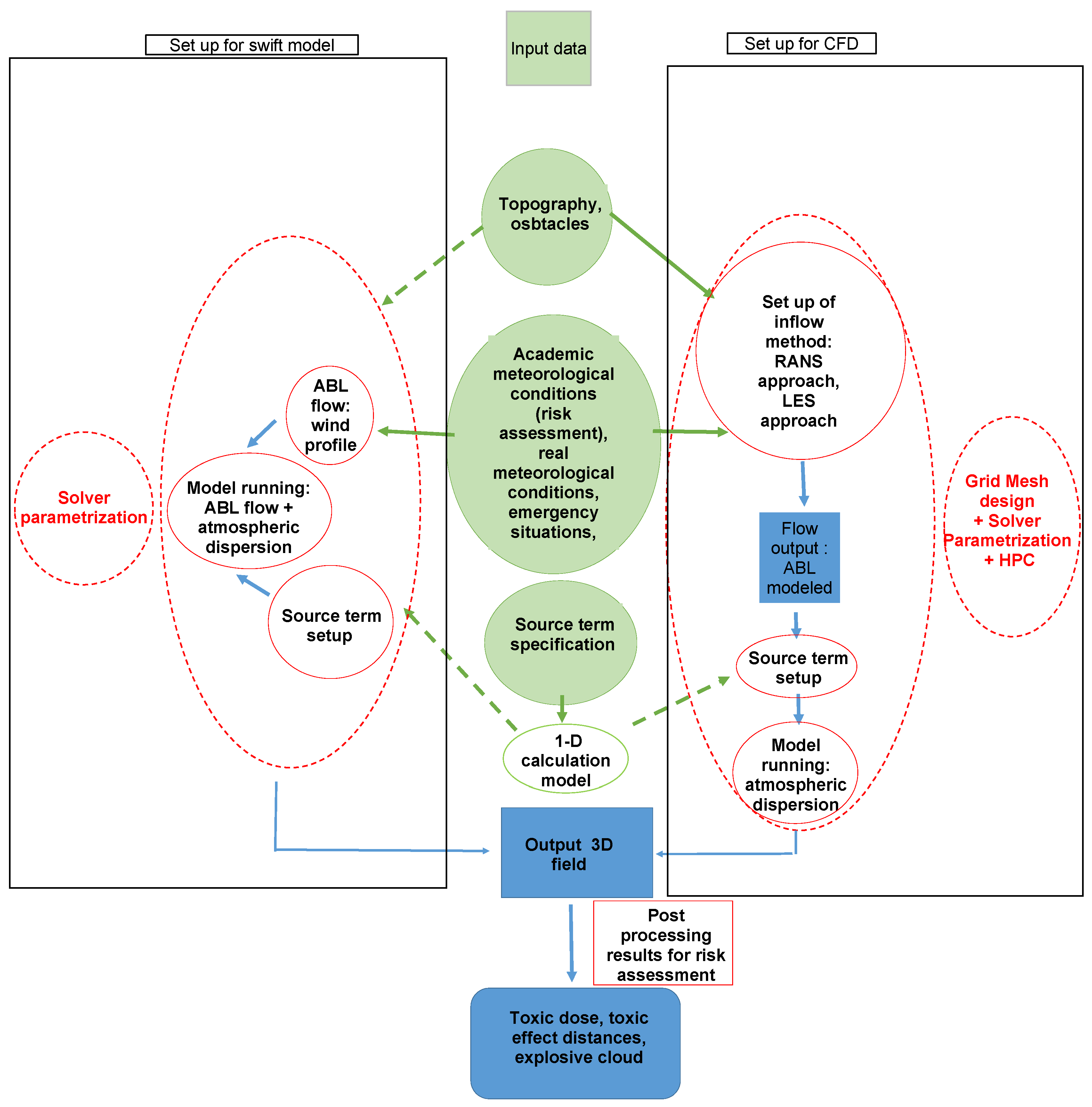
Figure 2.
Schematic view of the simplified source term for CFD approach for massive release studied in Section 3.
Figure 2.
Schematic view of the simplified source term for CFD approach for massive release studied in Section 3.
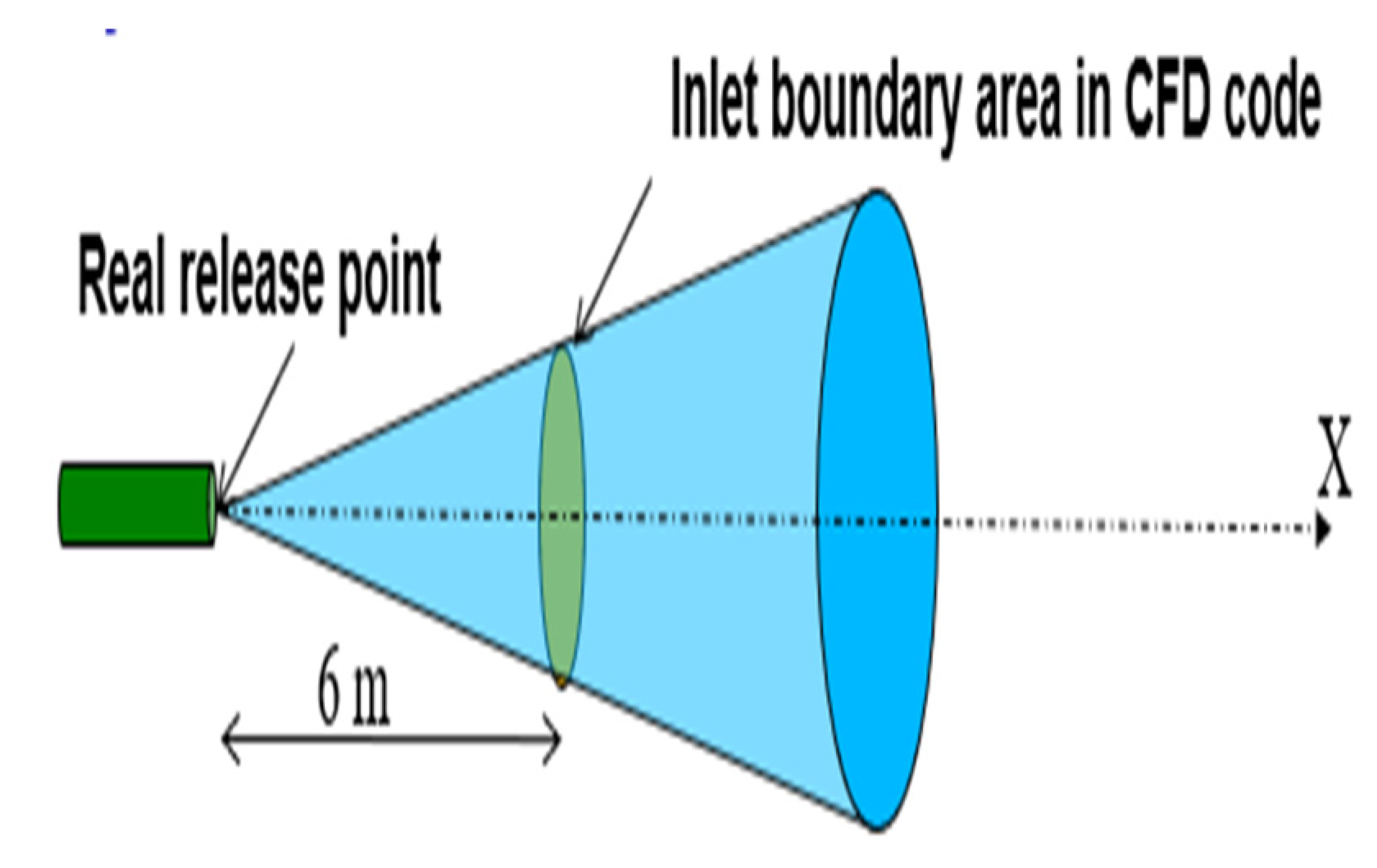
Figure 3.
The whole measurement area in CEA-CESTA for the ammonia experimental test cases; sensor arcs locations (distances from the release system: 20 m, 50 m, 100 m, 200 m, 500 m, 800 m and 1700 m for corresponding referenced letters A, B, C, D, E, F, G); mean wind direction of trial 4 is indicated by the blue arrow.
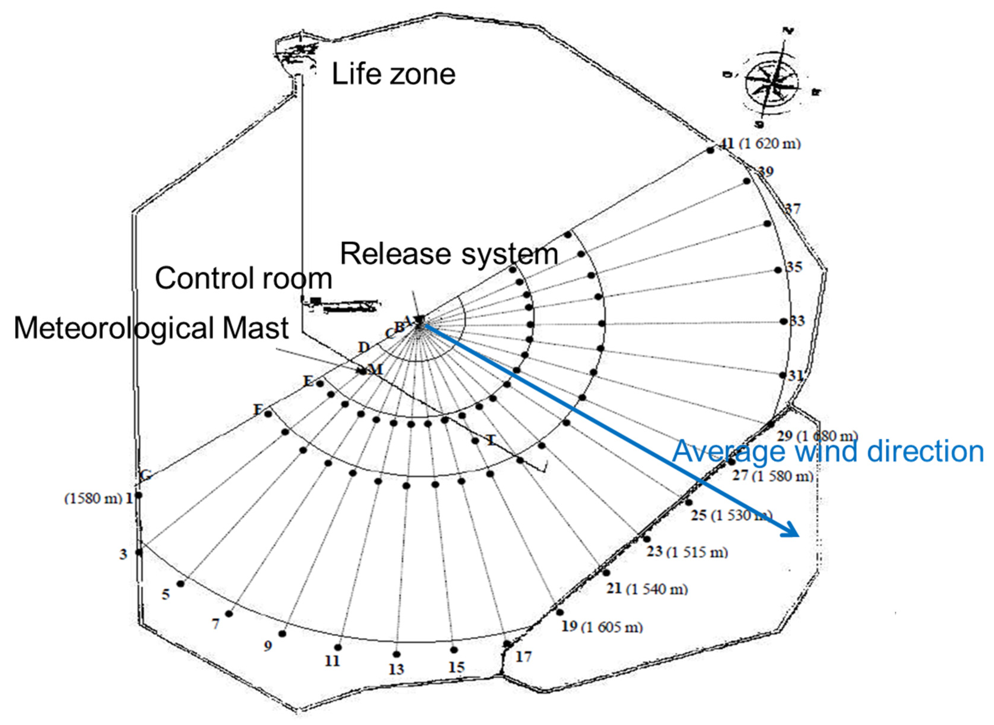
Figure 4.
Predicted results for the flow ABL profiles at the inlet (x=-100m), center and outlet of the domain with RANS CFD code.
Figure 4.
Predicted results for the flow ABL profiles at the inlet (x=-100m), center and outlet of the domain with RANS CFD code.
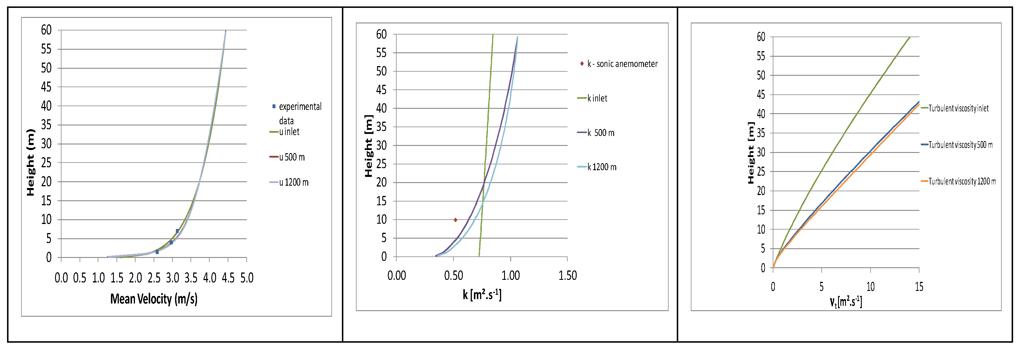
Figure 5.
Flow characteristics against inflow conditions (x=-100m) and experimental data - LES approach.
Figure 5.
Flow characteristics against inflow conditions (x=-100m) and experimental data - LES approach.
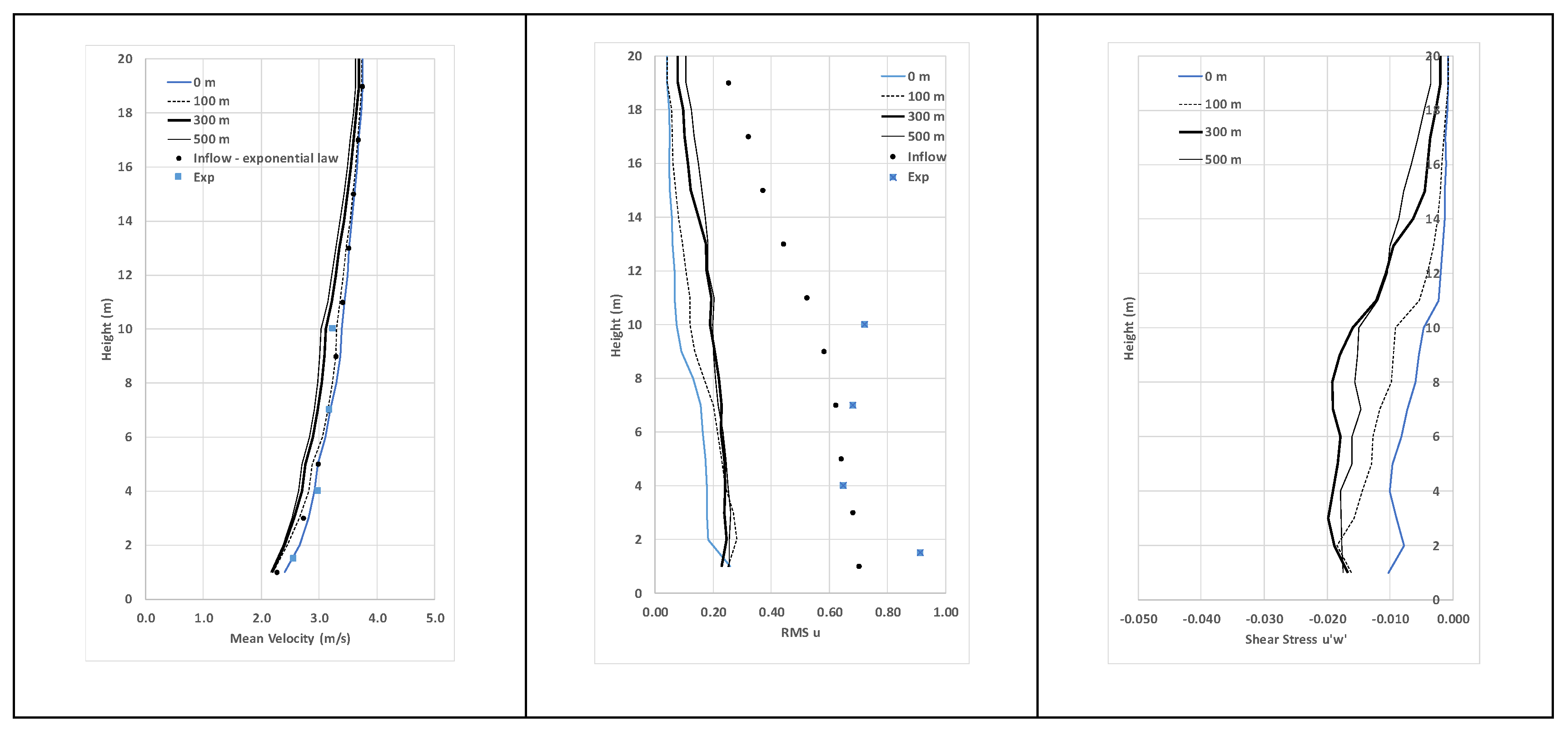
Figure 6.
Comparison between simulation results and maxima of experimental concentration for each sensors arc data.
Figure 6.
Comparison between simulation results and maxima of experimental concentration for each sensors arc data.
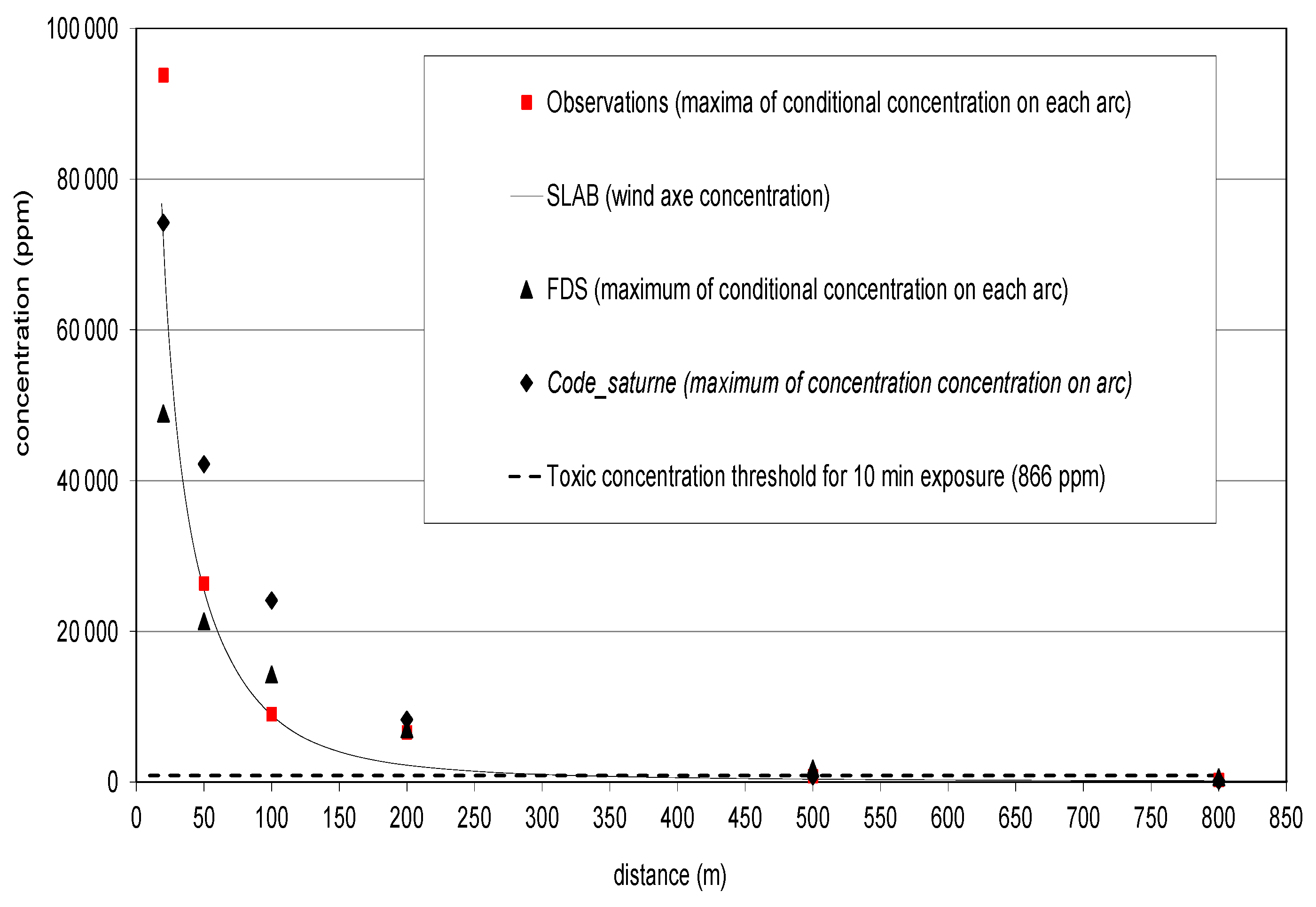
Figure 7.
Comparison between simulation results and experimental concentration data in the far field.
Figure 7.
Comparison between simulation results and experimental concentration data in the far field.
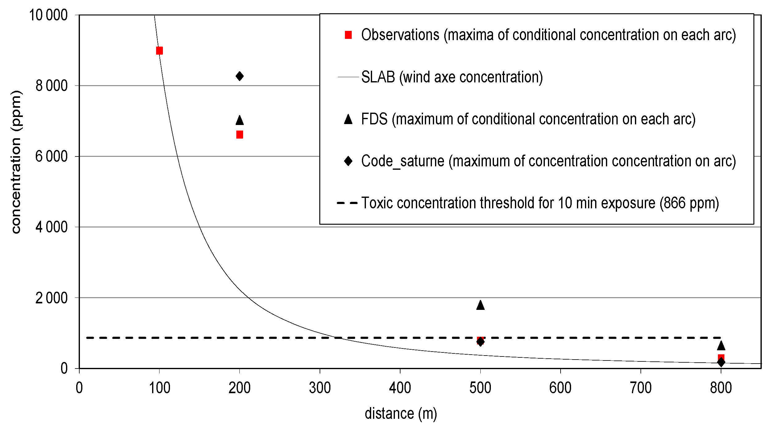
Figure 8.
comparison between the overall form of the experimental cloud shape and FDS simulation results: (a) photography of ammoniac cloud during trial 4 release; (b) iso-surface of ammonia simulated concentration (500 ppm).
Figure 8.
comparison between the overall form of the experimental cloud shape and FDS simulation results: (a) photography of ammoniac cloud during trial 4 release; (b) iso-surface of ammonia simulated concentration (500 ppm).
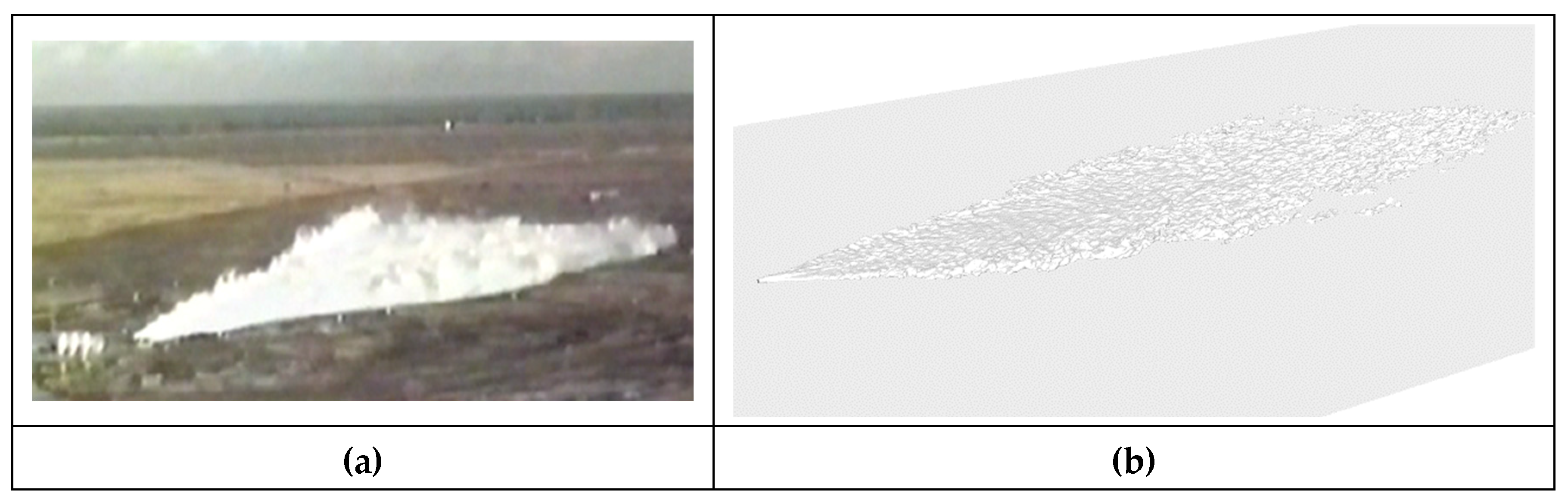

Table 1.
ultrasonic anemometer (10 Hz) measurements (over first 5 mins of the release) for trial case 4.
Table 1.
ultrasonic anemometer (10 Hz) measurements (over first 5 mins of the release) for trial case 4.
| Ambient temperature | wind speed (m/s) at 10 m | Friction velocity: u* (m/s) | Pasquill stability class by determined by the standard deviations of the wind direction |
Monin-Obukhov Lenght (LMO) (-) | |||
|---|---|---|---|---|---|---|---|
| 14.82°C | 3.24 | 0.36 | C | -166 |
Table 2.
Atmospheric input data for LES approach.
| Anemometer altitude (m) | Umean (m/s) | Tx (s) | Lx | RMSx |
| 1.5 | 2.59 | 12 | 31.0 | 0.72 |
| 4 | 2.94 | 14 | 41.1 | 0.68 |
| 7 | 3.18 | 20 | 63.6 | 0.64 |
| 10 | 3.24 | 17 | 55 | 0.9 |
Table 3.
Implementation of a Biphasic Dense Gas Source Term in CFD code: inlet boundary for CD code (a); characteristics of source term (b) determined by 1-D approach.
Table 3.
Implementation of a Biphasic Dense Gas Source Term in CFD code: inlet boundary for CD code (a); characteristics of source term (b) determined by 1-D approach.
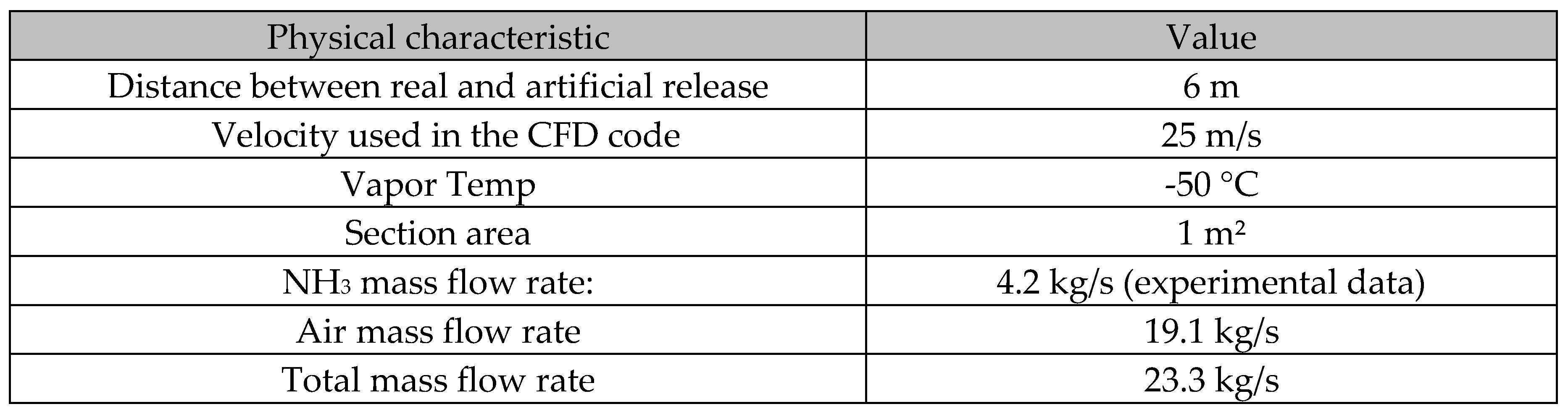 |
Table 4.
Harmonized and specific input data for SLAB model and CFD approach.
 |
Disclaimer/Publisher’s Note: The statements, opinions and data contained in all publications are solely those of the individual author(s) and contributor(s) and not of MDPI and/or the editor(s). MDPI and/or the editor(s) disclaim responsibility for any injury to people or property resulting from any ideas, methods, instructions or products referred to in the content. |
© 2023 by the authors. Licensee MDPI, Basel, Switzerland. This article is an open access article distributed under the terms and conditions of the Creative Commons Attribution (CC BY) license (http://creativecommons.org/licenses/by/4.0/).
Copyright: This open access article is published under a Creative Commons CC BY 4.0 license, which permit the free download, distribution, and reuse, provided that the author and preprint are cited in any reuse.


