Submitted:
03 January 2025
Posted:
07 January 2025
You are already at the latest version
Abstract
The Brazilian Forest Code regulates Permanent Preservation Areas (PPA) and Legal Reserves (LR) in all federation states. These areas support the maintenance of ecological functions and are essential for biodiversity conservation and environmental balance. However, their implementation faces significant challenges, especially in supporting agribusiness expansion, and their management is required for economic development while preserving natural habitats. Our study relies on data from the Rural Environmental Registry (RER), managed by the Brazilian Federal Government, to assess PPA and LR in São Paulo. We apply the geometric metrics Circularity Index, Edge Factor, Fractal Dimension, and Compactness Index to evaluate these protected areas’ shape and physical characteristics per singular and group of areas. The results highlight the correlation between the shape of these areas and their ecological functions, including their vulnerability to edge effects and habitat degradation. Moreover, the large-scale analysis correlating several areas revealed the complexity of these landscapes with different degrees of connectivity, vulnerability, and ecological efficiencies, assessing 645 districts. In conclusion, the results provide a framework for implementing protected areas that support ecosystem management and biodiversity conservation, particularly for enhancing agricultural productivity.
Keywords:
Brazilian Forest Code
; Protected Areas
; Geometric Metrics
; Biodiversity Conservation
; Sustainable Ecosystem
; Sustainable Agriculture
1. Introduction
Vegetation cover is critical in evaluating environmental quality and conserving ecosystems and habitats, enabling the sustainability of agricultural activities. Analyzing native vegetation, particularly its density and diversity, provides direct and reliable indicators of these aspects. Advanced technologies, likely remote sensing, have improved our understanding of ecosystem dynamics [1]. At the same time, approaches that leverage advanced computational tools offer deeper insights and customized solutions to complex environmental challenges. These methods facilitate continuous, large-scale monitoring, as emphasized by Forman (1995) [2] and corroborated by recent studies [3,4,5,31,32,33,34,35,37,38,41,42,43,46,47,53,55,56]. Therefore, these methods are a way to support the sustainability of agricultural and environmental management.
1.1. Protected Areas
Brazil’s Permanent Preservation Areas (PPA) and Legal Reserves (LR), established by the 2012 Forest Code (and updated in 2023), are essential to preserve vegetation cover and maintain environmental equilibrium 1. These areas ensure the protection of natural resources while supporting sustainable development for present and future generations. PPA protects vital natural features such as springs, riverbanks, and hillsides [4], whereas LR conserves native vegetation [4,5]. The Forest Code requires properties exceeding four fiscal modules to maintain LR and preserve vegetation in rural areas 2. This obligation can cover 35% of the property in the Cerrado-Savanna biome, 80% in the Legal Amazon Forest, and 20% in other areas specified by the Code.
Despite the robust conservation principles embedded in legislation, implementing and managing these areas, particularly within the agribusiness sector (a cornerstone of the Brazilian economy). With its continental dimensions and growing agricultural expansion, the country faces the challenge of balancing environmental conservation with economic development [5,6,7,8]. This scenario requires adopting strategies to safeguard biodiversity and promote the sustainability of agribusiness, especially in the continued expansion of agricultural activities. To address it, Brazil established the Rural Environmental Registry (RER) 3 platform to support the management and regularization of PPA and LR. This initiative marks a significant milestone in environmental management by integrating data on vegetation cover and land use, aiming to promote sustainability and the conservation of natural resources. Consistent with the principles of sustainable environmental planning outlined by Forman [2], the RER facilitates the environmental regularization of rural properties, ensuring legal compliance and supporting strategic decision-making.
The RER has become Brazil’s ecosystem management system, promoting biogeographic sustainability, enhancing environmental conservation, and supporting economic planning. By providing transparency and access to detailed information about rural properties, the platform enables monitoring of rural activities and identifies priority areas for conservation. This approach improves Brazil’s capacity to balance environmental stewardship with economic development. Moreover, the RER operates under Brazilian environmental legislation, establishing principles, rules, and standards for information registration. The Brazilian Ministry of the Environment stores the recorded data in the Rural Registry System (RER) 4, a centralized database. The public accessibility of this system ensures transparency for individuals, businesses, and researchers, providing vital information about rural properties and the surrounding environment. This openness promotes social accountability, supports scientific research, and enables decision-making for environmental conservation, positioning RER as a tool for participatory environmental management in Brazil.
Additionally, studies have emphasized specific methodologies for assessing protected areas using tailored metrics derived from RER data to analyze the functionality and effectiveness of these environments [9,10]. These approaches underscore the RER’s role in advancing conservation strategies, spatialization of legislation, and sustainable land management.
1.2. Related Works
Previous studies, like Laurance (2008) and Metzger (2013), have highlighted methodologies focused on analyzing protected areas [11,12]. However, applying these approaches in PPA and LR in Brazil has limitations, such as a lack of suitable metrics for Brazilian biomes. Moreover, Feng and Liu (2015) present a method to overcome these problems by providing a detailed analysis of these areas through geometric metrics [13]. It includes relevant information about environmental characteristics and their relationship with biodiversity conservation, translating it into mathematical models capable of quantifying values relevant to these issues. Analyzing the shape of these areas, for instance, enables the creation of indices and metrics to assess vulnerability to disturbances and compare different patterns across areas.
For example, elongated or irregularly shaped areas have a higher ratio of edge to interior, making them more susceptible to disturbances, known as the edge effect. This interaction can lead to negative consequences, like habitat degradation and the loss of species that depend on stable and undisturbed environments [14]. These conditions arise from changes in environmental factors at the edges of forest fragments, including increased sunlight exposure, wind, and temperature, as well as heightened vulnerability to invasive species and even fire events [15]. In Brazil, the edge effect may be intensified by the fragmentation of native ecosystems due to agricultural expansion and urban development, increasing the pressure on PPA and LR [16]. Analyzing the shape of PPA and LR contributes to understanding environmental dynamics and developing preservation strategies for these areas, facilitating the identification and implementation of management practices.
We can explore the complexity of PPA and LR shapes using the Area-Weighted Mean Patch Fractal Dimension (AWMPFD) [9,17]. This methodology, which will be utilized in this study, quantifies the diversity in the shape of vegetation fragments within a given area by considering the Area and Perimeter of each fragment. The complexity of these shapes, ranging from simple geometric forms to highly irregular ones, provides broader insights into the various landscapes found in Brazilian flora. This complexity impacts species movement and habitat connectivity [3,18].
Therefore, a set of metrics, including the Circularity Index (), Edge Factor (), Fractal Dimension (), and Compactness Index (), can be used for meeting functional expectations and assessing PPA and LR fragments. Together, these metrics allow for a quantitative analysis of the geometry of protected areas, providing relevant information about their physical characteristics and how these might affect biodiversity within habitats [9,17].
1.3. Geoprocessing Techniques
Geospatial analysis tools, like Geographic Information Systems (GIS), are employed to interpret data focusing on the Earth’s surface and physical aspects. GIS allows for collecting, organizing, analyzing, and visualizing geographic locations and environmental concerns. These systems enable a detailed understanding of the environment by connecting maps and coordinates with information such as population data, climate, and environmental balance [17,33]. GIS systems integrate various concepts into a single platform, providing a pathway to investigate relationships between local spaces and phenomena such as environmental changes, species movement, and geometric metrics. GIS facilitates analyses that reveal patterns and effectively support decision-making processes, clarifying complex issues.
Thus, GIS tools are suited for analyzing PPA and LR available on the Rural Registry System platform. The data is provided in “.shp” format, or Shapefile, and is used in GIS technologies employing vector geospatial data. This vector data is represented as Points for locating specific positions, Lines for features like rivers and access roads, and Polygons to define areas such as forests, fields, or plantations, representing the geometry of a specific region [33]. Within this classification, two or more polygons are one multi-polygon. The difference lies in the structure and type of area each represents:
- A polygon is a single closed area formed by a sequence of connected points (edges) that form its contour. The starting and ending points must coincide to close the shape. Polygons can have holes within them, defining empty areas, such as islands within a lake.
- A multi-polygon combines multiple polygons representing complex areas composed of several distinct polygons [34].
Therefore, GIS tools and data are useful for analyzing PPA and LR, offering capabilities to understand and manage these protected areas.
1.4. Objectives and Hypothesis
The increasing pressure from agricultural and urban expansion on Brazilian ecosystems makes the conservation of biodiversity and the maintenance of ecosystem services an urgent priority. PPA and LR are fundamental for safeguarding habitats, protecting water resources, and mitigating climate change. Assessing these protected areas’ complexity is essential to understanding their spatial configuration and ensuring the long-term integrity of these ecosystems. Using metrics provides insights into these areas’ complexity and spatial organization, enabling the identification of distribution patterns and vulnerabilities. Thus, we proposed an approach to manage these areas effectively, providing an understanding of their spatial dynamics. This research seeks to improve strategies for sustainable development in Brazil, offering insights that can benefit other nations facing similar challenges.
In this context, our approach employs environmental metrics and RER’s data to analyze the spatial configuration of PPA and LR in São Paulo State, providing a quantitative foundation for monitoring and management strategies to support decision-making processes. Additionally, the research aims to develop a methodology for geospatial processing and analysis of PPA and LR, contributing to improving computational prototypes and their representation. The long-term goal is to enhance public policies, promote sustainable management, and position Brazil as a global leader in biodiversity conservation. We hypothesize that geometric metrics and the RER dataset can support the management of PPA and LR by identifying the complexity of the behavior of these areas in space and time dynamics.
Thus, this paper follows a standard structure. The Introduction provides context, emphasizing the importance of spatial analysis in environmental management using RER (Rural Environmental Registry) data. The Materials and Methods (Section 2) describe the datasets and the metrics applied. The Results and Discussion (Section 3) highlight key spatial patterns and their implications. The Conclusions and Further Work (Section 4) summarize the contributions and propose future research directions to refine methods and expand datasets.
2. Materials and Methods
This study evaluates the effectiveness of the Brazilian Forest Code in protecting native vegetation by analyzing the spatial organization of PPA and LR using quantitative methods. Our methodology used RER (Rural Environmental Registry) data, incorporating key categories such as Consolidated Area, Hydrography, Polygon Map, Permanent Preservation, and Legal Reserve. To assess spatial characteristics, we apply metrics including the Circularity Index (), Edge Factor (), Fractal Dimension (), and Compactness Index (). These metrics are used to evaluate both individual areas and groups of areas, enabling the identification of individual and overall patterns. Our approach provides insights into spatial organization, structural characteristics, and the relationships between areas within the specified categories. Also, we use the numerical data generated for statistical analysis and computational modeling to assess the shape and fragmentation of the areas [35].
2.1. Circularity Index ()
The Circularity Index () is used to quantify the shape of the area. The geometric relationships of these areas contain valuable information for interpreting their effects. The compactness of an area is often related to its ability to protect its interior from external influences. Circular-shaped fragments are considered ideal in environmental terms as they minimize edge effects, which amplify external influences such as strong winds, invasive species, and microclimatic changes [19]. is a widely used metric for measuring the geometric regularity of an area, with a circle being the most compact shape possible. Areas with more elongated or irregular shapes tend to have a higher edge-to-interior ratio, making them more susceptible to environmental disturbances and the loss of interior-dependent species [20,21].
The Equation (Equation 2.1) correlates the area of the observed shape with that of a corresponding circle, indicating how closely the shape of an area aligns with a perfect circle. Values range from 0 to 1, where values near 1 indicate more circular shapes, while values closer to 0 indicate more irregular or elongated shapes. Equation 2.1 expresses the circularity () measured between the area of the shape and the area of a circle with the same perimeter, as given by Equation 2.1:
Where:
- is a Real Area representing the shape’s area under analysis. It is the total surface area of the shape, typically expressed in square units (e.g., square meters for physical areas).
- is the area of the ideal circle with the same perimeter as the analyzed shape (e.g., meters).
- is the actual Real Perimeter of the shape, i.e., the total measurement along the real boundary of the analyzed area. This perimeter is measured in linear units (e.g., meters) and reflects the true extent of the shape’s edge, including any irregularities or fragmentations.
2.2. Patton Diversity or Edge Factor ()
The Edge Factor (), also known as Patton Diversity, is another metric used to quantify the irregularity of the edges of a protected area. Areas with more irregular edges tend to have greater exposure to edge effects, which can hinder habitat connectivity and increase the ecosystem’s vulnerability to external disturbances [22]. This index is used to assess the irregularity of the boundaries of a geographic area, such as a conservation unit or any other region [23]. Areas with more irregular, curved, or thinner boundaries tend to exhibit higher Patton Diversity values, indicating that the shape is less efficient in terms of perimeter relative to the area it occupies. The higher the value, the more complex the evaluated area. quantifies the perimeter’s irregularity relative to the shape’s area. It is calculated as the ratio between the actual perimeter () and the expected perimeter for an ideal geometric shape with the same area (). A value of greater than 1 indicates a more irregular or fragmented edge, while values close to 1 indicate a more regular and smooth edge. The formula is represented in Equation 2.2:
2.3. Fractal Dimension ()
A detailed analysis of fractal sets can provide a quantitative measure of the geometric complexity of natural area boundaries [17,24,25]. Fractal Dimension refers to the ability to evaluate an area’s spatial characteristics, such as vegetation patches, and how they behave regarding potential irregularities or complexities [21,26]. A fractal is related to the measurement of the geometric complexity of an area. Areas with high fractal complexity are more fragmented and exhibit more irregular shapes, which can hinder species movement and the maintenance of habitat connectivity [21,27]. It allows for analyzing spatial patterns at multiple scales, providing valuable insights into geospatial resilience and the long-term impacts of fragmentation [9]. This metric can reveal necessary information about the relationship between the shape of areas and their habitat resilience. For instance, areas with higher fractal dimensions may have more irregular edges, affecting species distribution and ecosystem dynamics. In other words, higher fractal dimension values may indicate complex structures that suggest increased vulnerability [21].
The fractal dimension measures how the perimeter of a shape increases relative to its area. The logarithmic function used to capture this relationship is suitable for linearizing the nonlinear relationship between perimeter and area, enabling the calculation of fractal complexity. A higher fractal dimension indicates greater complexity or irregularity. Values range from 1 to 2, with values closer to 2 indicating more complex shapes and those closer to 1 indicating simpler shapes. Equation 2.3 relates the fractal dimension to the perimeter and its area:
2.4. Compactness Index ()
The Compactness Index is similar to the Circularity Index but provides a more precise measurement by analyzing the relationship between the perimeter of an area and its spatial efficiency [28]. The closer the Compactness Index is to 1, the more compact the area is, indicating less exposure to external influences such as invasive species or microclimates, which are more intense along the edges of fragmented areas [17,29,30], and more recent studies [31,32]. When approaches 1, the shape has a more efficient configuration with less irregularity in space along its perimeter, indicating more compact shapes and closer to a circle.
In the Compactness Index (), the following variables are represented in Equation 2.4:
This index effectively highlights the spatial efficiency of a shape, with higher values indicating more compact configurations, reducing exposure to edge effects and enhancing ecological resilience. It is important to note that the results of the Metric calculations are obtained based on the Real Perimeter (PR) and Real Area (AR), whose values are collected in the data acquisition process performed during the processing of the shapefiles. In this way, the transversal calculations are eliminated, and the metrics are determined by convolution.
Table 1 summarizes key metrics used in evaluating geospatial forms, highlighting their purpose in environmental analysis. The Circularity Index () measures shape compactness, with values near 1, indicating minimal edge effects and enhanced suitability for biodiversity conservation, while irregular shapes are more prone to external disturbances. The Edge Factor () assesses edge irregularity, with higher values signaling fragmented shapes that may require targeted conservation efforts. The Fractal Dimension () quantifies geometric complexity, enabling multi-scale analysis of spatial patterns to understand ecosystem resilience and dynamics. Finally, the Compactness Index () evaluates an area’s exposure to edge effects, where shapes approximating a circle demonstrate superior ecological efficiency by protecting their interiors. These metrics provide a comprehensive toolkit for spatial analysis, aiding in identifying vulnerabilities and conservation priorities.
2.5. Dataset Source
The state of São Paulo was selected as the study area because its intense agricultural and industrial activity provides a context for analyzing the implementation of the Brazilian Forest Code. This characteristic makes the state relevant, especially in balancing agricultural production and environmental conservation challenges. As mentioned, this study will utilize RER data, focusing on PPA and LR’s spatial characteristics. São Paulo has approximately 439 thousand rural properties registered in RER. The vector data (.shp) required for the analysis were sourced from RER. Among the areas registered in RER in São Paulo, 7 thousand PPA polygons totaling approximately ha and 100 thousand LR totaling ha were analyzed, as described in Table 2. Each polygon represents a PPA or LR area associated with a rural property registered in RER.
The areas associated with PPA are often registered in the RER in a segmented manner, consisting of small parts that, when combined, form the Total PPA. The Total PPA represents the total area of permanent preservation associated with a rural property consisting of one or more segments. We chose this structure to avoid generating trends in the indicators, as analyzing each segment could lead to biased results due to its small area and irregular shape. The PPA registry contains approximately million segments across 90 thousand total PPA, from which we selected 7 thousand Shapes for analysis. The coordinate system was the EPSG:31983 - SIRGAS 2000 / UTM zone 23S. This spatial reference system uses the SIRGAS 2000 datum, officially adopted in Brazil, and is particularly suitable for representing geospatial data in a large part of the state of São Paulo. This study focuses primarily on analyzing all selected areas of the polygon type to avoid creating trends in the data sample. Data processing was performed using the Python programming language in conjunction with some specific geoprocessing libraries (GeoPandas 5, Shapely 6), to obtain the results inherent to the processing of specific data, like the use of shapefiles, which the system can easily manipulate and analyze the spatial geometry in greater depth and visualize the results. The QGIS tool was also used to view maps, geospatial information, point extraction, and feature selection.
2.6. Data Collection, Geometric and Spatial Analysis
This study used vector data from the Brazilian Institute of Geography and Statistics (IBGE) 7, the Brazilian Forest Service (SFB) 8, and local environmental agencies, which were also surveyed for information on tropical forests [36]. As mentioned, the primary data source was shapefiles from the Rural Registry System platform. We based the geospatial analysis of the geometric shapes of PPA and LR on these data.
2.7. Data Acquisition Process
The information in the RER shapefiles had to undergo a specific data-cleaning process to address only the issues useful to the applications. It involved a series of steps, as the data for a registered property contains much information about the rural property that was unnecessary for this project. Figure 1 illustrates the steps, from acquiring the information to processing the data.
The following procedure is described in Table 3 for obtaining spectral image shapefile data to perform a quantitative analysis of desired location fragments of the habitat of a region or vegetation of interest.
The shapefiles obtained from the RER were processed using programs developed in Python. It allowed data integration, enabling simulation to calculate spatial metrics applied to the PPA and LR Areas. The processing sequence described in Table 3 details the step-by-step process, from data filtering to the generation of geometric metrics, like area, perimeter, circularity (), edge factor (), fractal dimension (), and compactness index (). After calculating the metric parameters for all fragments, we organized the data to analyze and identify patterns in fragment shapes and their relationships, enabling the exploration of edge effects.
2.8. Geospatial Computational Analysis
We integrate data science and geospatial analysis to investigate the distribution patterns and configurations of Permanent Preservation Areas (PPA) and Legal Reserves (LR) in São Paulo. We processed data using Python with libraries including GeoPandas, Pandas, NumPy, Shapely, Matplotlib, and Scikit-learn. We also used the GeoPandas library to process geospatial data. It expands the functionalities of Pandas, adding support for geographic information, like points, lines, and polygons. GeoPandas introduces the concept of a GeoDataFrame, enabling geographic data to be stored in a specialized column called Geometry. We use the Shapely library to extract information about geographic shapes. It allows for the calculation of areas and distances, the creation of buffers, and the performance of intersections between shapes, just a few functions. In Geopandas, we can work with spatial files, such as shapefiles, GeoJSON, and KML. The MatplotLib library was essential for creating the graphs. The Pandas and NumPy libraries were necessary for working with the data and statistical calculations.
Besides, we used the k-Means algorithm in the exploratory analysis to identify patterns, as the LR and PPA datasets are large. The main objective was to create several clusters to obtain the respective data sets. The most commonly used library to work with the k-Means algorithm in Python is Scikit-learn. The objective is to evolve to use predictive analysis models, which allow the simulation of future scenarios, projecting the development of ecosystems or identifying problems that can be avoided, such as inappropriate land use and other unwanted changes. These models provide strategic support for decision-making aimed at environmental conservation, helping to implement more effective preservation policies and actions.
2.9. Computer Simulation Equipment
This research was supported by the High Performance Computing Center of the Federal University of Pará (CCAD - UFPA). The processing and analysis of the extensive volumes of geospatial data and the execution of the required complex computer simulations were performed using the Apolo 2000 supercomputer, CCAD - UFPA. This equipment is part of the National High-Performance Processing System (SINAPAD), an initiative of Brazil’s Ministry of Science, Technology, and Innovation (MCTI) 9. This equipment, HPE (Hewlett Packard Enterprise), has 31 computing nodes, each equipped with two Intel Xeon 6132 14-core processors, totaling 868 processing cores. In addition, the Apollo 2000 has 3,392 GB of RAM, 156 TB of storage, and an NVIDIA Tesla V100 GPU with 512 GB of dedicated memory, reaching a processing capacity of approximately 8.0 TFlops with 90% efficiency.
Regarding data processing, a high-performance statistical analysis was performed to assess the consistency of the information related to the records using high-performance processing. It is important to highlight that some critical aspects added to the interpretation of the results justify the need for high computational capacity since there is a need to guarantee the reliability of the information. This data reflects the variation in the shape of the fragments with the size of the areas; this quantity encompasses many vector polygons extracted from the RER shapefiles. Each of these polygons underwent geometric refinement. The Apollo supercomputer processing calculated the metrics for a huge set of fragments, each with variations in area, perimeter, circularity, and edge complexity. These calculations are computationally intensive, especially for larger and more complex fragments, which require more processing power due to their complex geometry.
2.10. K-Means for Data Classification
Classification techniques, specifically k-Means, were used to analyze the resulting data. It was done to identify structures and patterns that could be hidden. The reason for grouping and classifying is to look for correlations to identify general patterns between them to simplify the interpretation of the data. Or even to identify redundant variables, in which clusters with high correlation can be indicated in the variables that are essentially measuring the same construct, which is very useful for reducing the dimensionality of the data. Another advantage would be discovering unexpected correlations in the relationships between variables that were not obvious initially, making it possible to generate hypotheses that can suggest new ideas and directions for future research [37,38].
As shown in Figure 2, each subplot highlights the composition and spread of elements within individual clusters. Cluster 2 shows a sparse distribution with a few isolated elements, while Cluster 5 exhibits a denser distribution with a concentration of elements along a primary axis. Cluster 6 demonstrates a balanced spread with distinct groupings, whereas Cluster 7 shows a wider range of element placements with higher variability. Using exponential scaling enables a clear representation of subtle differences in element positions and densities across clusters.
3. Results and Discussion
The results obtained in the analysis of Permanent Preservation Areas (PPA) and Legal Reserves (LR) were analyzed by applying quantitative metrics: (Circularity Index), (Edge Factor), (Fractal Dimension), (Compactness Index) (Section 2). This approach allows a targeted characterization, focusing directly on the quantitative analysis of spatial data and numerically evaluating these protected areas’ degree of fragmentation and spatial integrity.
3.1. Sample Size
In São Paulo, properties used for agricultural activities were registered, covering ha. Of this area, ha are earmarked for preservation and represent approximately of the total area of rural properties in the state [42]. In the state of São Paulo, legislation requires that of the area of each rural property be set aside for LR. According to the state’s Rural Registry System data, around LRs and PPAs are registered. This research used approximately LRs and PPAs, analyzing around ha of PPA and LR. Table 4 provides more detailed information on using this data.
For the LR studied, the average is ha compared to for the PPA. This difference in size is mainly due to federal environmental legislation (by the Brazilian Forest Code), which defines LR as a higher mandatory percentage of the total area of rural properties than PPA. PPA, however, are delimited by specific criteria, such as a preservation area relating to watercourses, springs, and hilltops, and are not directly linked to the property’s total area. This pattern highlights the predominance of smaller areas among PPA. According to Schober (2018) [43], the differences and variations reported in the quantity and size of areas can have significant geospatial implications. In environmental terms, smaller areas suggest a lower concentration of vegetation and are potentially vulnerable regarding their ecological functionality. Preserved areas of small size generally show less resilience to disturbance and less effectiveness in conserving biodiversity, especially for species that require extensive and connected habitats.
Figure 3 (a) shows the size distribution of the PPA. One highlight is the asymmetrical distribution to the left in the corresponding histogram, indicating a greater concentration of smaller fragments. In particular, the peak of the histogram reveals that most of the fragments have areas of less than 5 ha. This pattern suggests that areas with more irregular configurations could benefit from specific management interventions, such as implementing buffer zones to reduce edge effects. The asymmetry observed in the distribution of LR in Figure 3 (b) is similar to the pattern found in PPAs, suggesting that these areas are larger. The histogram shows a higher concentration in fragments of up to 11 ha. Larger fragments, over ha, are fewer in number, with decreasing frequencies as they increase in size. The logarithmic scale in the frequency highlights the contrast between the number of small and large fragments, reinforcing the predominance of the smaller ones.
3.2. Results on Information of PPA and LR Data
Table 4 describes the two datasets, which include vector polygons obtained from the Rural Registry System (Section 1). This universe corresponds to PPA and LR.
It is possible to observe a high variability in the sizes of these areas, especially in LR. The initial analysis identifies an average area of ha per PPA and ha per LR, which reflects the differences in regulations and specific conservation objectives. The histograms in Figure 3 (a, b) show the distribution of the areas studied in PPA and LR. They reveal a significant difference between the sizes present in these areas. PPA mostly presents smaller fragments, while LR exhibits high variability with continuous fragments, as observed in the concentration of fragments of different sizes.
The histograms illustrate the distribution of areas for PPA and LR on a logarithmic scale. PPA are predominantly small, with most areas under 20 ha and a sharp decline in frequency as area increases, indicating rare occurrences of larger PPA (up to 100 ha). In contrast, LR exhibits high variability, with most areas below ha and some extending to . The skewed distributions of PPA and LR highlight the dominance of smaller areas, while larger ones are less frequent. This pattern reflects the distinct spatial characteristics of these areas, with PPA generally being smaller and more uniform. In contrast, LR shows a broader range, offering insights into their ecological functions and informing conservation efforts [17].
3.3. Geospatial Data Sample Results
Figure 4 presents examples of PPA and LR geospatial fragments, highlighted in Figure 3 (a, b). They illustrate the spatial distribution of areas in São Paulo, highlighting the differences in shapes and sizes between PPA and LR. This spatial characterization is essential for the analysis and interpretation of the results. Computational refinement eliminated small redundant areas and corrected topological errors to ensure integrity and accuracy. We randomly selected all areas from this set. This process removed overlaps, corrected gaps, and eliminated invalid polygons, significantly reducing geometric inconsistencies. In this way, we improved the quality of the input data for mathematical modeling and subsequent metrics calculations. This preprocessing aimed to ensure the accuracy of the geometric complexity of the areas studied. The fragments of the selected study areas are presented in Tables Table 4 and Table 5, subdivided into two main categories (PPA and LR) so that we could monitor the procedures carried out during the information collection stage.
Table 5 presents two fragments of selected PPA (forms A and B), while Table Table 5 shows two LR (forms C and D), displaying the geometric differences between the fragments. Each fragment presents its corresponding metrics and indexes, (), (), (), and (), to characterize the degree of fragmentation and spatial configuration of these sites.
Fragment A, Table 5, has a total area of ha and a perimeter of meters. We can observe a highly regular shape, with a Circularity Index () close to 1, suggesting an almost circular appearance. This regularity is confirmed by the Edge Factor (), indicating well-defined and simple edges, and by the Fractal Dimension (), which reflects the average geometric complexity. The Compactness Index () also presents a geometry close to a circle with a value close to 1.
However, Fragment B, Table 5, presents a less regular shape, with a total area of ha and a perimeter of meters, with a Circularity Index (), suggesting a more irregular shape. The Edge Factor () and the Fractal Dimension () indicate a more complex edge and a more fragmented geometric configuration than Fragment A, as also shown by the Compactness Index (). It is interesting to observe large differences in the shapes of these fragments and how they are reflected in the metric values. In Table 5, two fragments of selected LR can be observed. Similarly, the images highlight each fragment’s shape and perimeter, representing the geometric variability in the analyzed areas and their metrics.
The first fragment analyzed is an LR (Fragment C), with a total area of ha and a perimeter of meters (Table 6). It is characterized by a highly irregular shape, with a Circularity Index (), indicating low circularity and a more elongated shape. The Edge Factor () suggests a complex and fragmented edge, while the Fractal Dimension () reveals high geometric complexity, reflecting the irregularities of the edges and shape (). Fragment D, Table 6, in turn, is also an LR with a total area of ha and a perimeter of meters and has a more compact shape, with a Circularity Index (), presenting a slightly more regular shape than Fragment C. However, there are still irregularities, such as the edge factor (), the fractal dimension (), and the compactness index (), indicating moderate complexity and less complexity at the edges.
The data generated by the computational extractions and applied to the selected fragments were compiled and summarized in Table 7. It presents a comparative relationship between the fragments considered and their diversity in sizes and shapes, revealing numbers related to their characteristics. Correlations can be observed between the contours and outlines of shapes and the quantitative representation of their geometric attributes. For instance, as in , values approaching correspond to shapes with circular characteristics.
Table 7 compares measured factors (area and perimeter) and calculated parameters (Circularity Index, Edge Factor, Fractal Dimension, and Compactness Index) for four fragments categorized as Permanent Preservation Areas (PPA) and Legal Reserves (LR). PPA generally exhibits higher circularity and compactness, with Fragment A being the most circular and compact (, ) despite having a large perimeter relative to its small area. In contrast, LR shows greater variability in shape and complexity, as evidenced by their lower circularity and compactness indices but higher edge factors and fractal dimensions, with Fragment C being the most irregular. These differences highlight distinct spatial characteristics between PPA and LR, which are critical for understanding their ecological functions and guiding conservation efforts [17].
3.4. Data Obtained from Shape Refinement in PPA and LR Metrics
The volume of data obtained and the geometric complexity of these areas justify the need for larger segmentations to ensure that the calculated metrics reflect the spatial characteristics of the set. Regarding PPA, of the fragments, as shown in the histogram in Figure 3 (a), are located below areas with around to 5 ha. Since the histogram shows a logarithmic relationship, approximately 6 thousand properties (approximately ) are in this range. Therefore, Table 8 shows the results of the area segments of these groups of fragments in three distinct size classes: (S) small fragments in the range up to ha, (M) medium fragments of to 20 ha and (L) large fragments equal to or greater than 20 ha, according to the histogram in Figure 3 (a). In this way, it was possible to reconcile the distribution of areas to assess this set’s distribution better.
The segmentation results for the PPA are reproduced in Table 9, which presents the statistical values of the metrics studied (, , , and ), distributed according to the segmentation in Table 9. The mean values, median, mode, variance, standard deviation, standard error, and other statistics for each set of classes are briefly demonstrated.
The segmentation of PPA areas into distinct size classes aimed to facilitate the analysis of their spatial distribution and associated metrics. Based on the histogram in Figure 3 (a), the majority (approximately ) of PPA fragments have areas smaller than ha (classified as small, S). A smaller proportion of fragments (about ) fall within the range of to 20 hectares (medium, M), and only are larger than 20 ha (large, L), as detailed in Table 8. This classification allows for a more precise examination of how fragment size correlates with geometric metrics (, , , and ). For instance, smaller fragments (S) typically exhibit lower compactness () and higher edge factors (), reflecting their susceptibility to external pressures such as edge effects and microclimatic variations. In contrast, larger fragments (L) tend to have greater compactness and lower edge factors, suggesting better interior habitat conditions.
Table 9 provides statistical summaries of these metrics, including the mean, median, and variance across the three size categories. The segmentation and resulting metrics underscore the ecological importance of addressing the vulnerabilities of smaller fragments. Restoration efforts and the creation of ecological corridors could mitigate their exposure to edge effects, while large fragments should be prioritized for strict preservation to maintain their ecological integrity. It should also be recognized that the high proportion of smaller and irregular PPA fragments (those with sizes ( ha) highlights significant ecological challenges. These areas, characterized by low compaction () and high edge factors (), are more susceptible to edge effects, such as increased exposure to sunlight, wind penetration, and temperature fluctuations. These conditions can degrade habitat quality, reduce biodiversity, and increase vulnerability to invasive species. In contrast, larger and more compact fragments ( ha) demonstrate greater ecological stability, as indicated by their higher compactness () and lower edge factors (). These fragments are more suitable for interior-dependent species and more resilient to external pressures. However, the small number of these larger fragments () highlights the need for targeted conservation efforts to protect and expand these critical areas.
Moreover, the LR segmentation follows the same organization and the order of the values proposed for the PPA areas. In this case, the histogram in Figure 3 (b) contains approximately properties, corresponding to of the total, within the range of up to 15 ha, and a smaller range indicated in the histogram contains properties of approximately 200 ha. Table 10 shows the area segments in 3 distinct size classes: (S) small fragments in the range of up to 11 ha, (M) medium fragments from 11 to 70 ha, and (L) large fragments equal to or greater than 70 ha, according to the histogram in Figure 3 (b).
Similarly, the results of the refinements for the LR are in Table 10. The statistical results of the metrics studied (, , , and ) are subdivided into classes, as described in Table 10. Table 11 presents the mean values, median, mode, variance, standard deviation, standard error, and other statistics for each set of classes.
The analysis of the LR dataset highlights significant ecological patterns across the 3 size classes: Small (S), Medium (M), and Large (L), Table 10. For the , small fragments (mean ) exhibit higher variability, as reflected by their standard deviation , indicating that these fragments are more prone to fragmentation effects. As shown in Table 11, medium fragments mean show intermediate compactness, while large fragments mean maintain slightly lower compactness. Despite this, larger fragments benefit from their size, offering better ecological stability.
The reveals heightened vulnerability for all size classes, with small fragments showing a mean of . This suggests a significant exposure to external pressures such as sunlight, temperature fluctuations, and invasive species. Medium fragments have the highest mean of , indicating they are the most susceptible to edge effects. Large fragments also exhibit considerable edge exposure mean , likely due to irregular shapes or high perimeter-to-area ratios, despite their size advantage. Regarding the , small fragments (mean ) tend to have simpler, less complex boundaries, whereas medium fragments mean and large fragments mean display decreasing boundary complexity. This pattern reflects increasing regularity in shape as fragment size increases, which enhances ecological resilience. The further underscores this trend, with small fragments (mean ) maintaining greater shape regularity. In contrast, medium mean and large mean fragments exhibit slightly lower compactness, possibly due to fragmentation or irregularity in shape. Figure 5 shows the mean of each size and type for metrics.
Ecologically, small fragments are particularly vulnerable due to their high edge factors and moderate compactness, which expose them to habitat degradation, reduced biodiversity, and increased risk of invasive species [17]. Restoration efforts, such as creating ecological corridors, are crucial to mitigate these vulnerabilities. Medium fragments, despite their larger size, face the highest edge-related pressures and require strategic preservation measures to enhance their stability. Large fragments, while relatively more stable due to their size, still experience significant edge effects, emphasizing the need for strict conservation and restoration practices to maintain their ecological integrity. Overall, the LR dataset highlights the critical importance of targeted interventions to preserve and restore habitat quality across all fragment sizes. The implications of these findings suggest that restoration strategies, such as creating buffer zones and ecological corridors, are essential to increase connectivity between smaller fragments and mitigate edge effects. Ecological functionality and landscape resilience can be significantly improved by integrating these approaches.
3.5. Analysis of Connectivity and Fragmentation in PPA and LR
The analysis of PPA revealed that most fragments have high , suggesting the need for interventions to restore or connect these areas. The high fragmentation (many small fragments) indicates that lacking geospatial connectivity may hamper PPA. It could jeopardize their function of protecting biodiversity and ecosystems since smaller fragments tend to be less resilient to environmental disturbances. Despite the limitation of the Fractal Dimension mentioned by Loke & Chisholm (2022) [47], the in our article proved to be a similarity metric for assessing the geometric complexity of fragments. Imre and Bogaert (2004) [21] mentioned complex shapes, , and metrics in fragmented property areas and compared area and perimeter for the geospatial index. serves as a key metric for assessing geometric complexity. Higher values indicate fragmented forms that can impede species movement and connectivity. In our analysis, areas with high are associated with greater geospatial vulnerability, suggesting that intensive management strategies are needed.
Furthermore, smaller fragments may indicate a more dispersed and fragmented implementation of PPA, which may require more specific geospatial restoration policies and linking these areas through corridors or connecting habitats [47]. The high fragmentation revealed in this PPA survey highlights the need for policy and restoration interventions to increase connectivity between fragments, allowing these areas to fulfill their geospatial functions more effectively. Research shows that habitat division disproportionately impacts the ecosystem services provided by conservation areas such as PPA, such as water resource protection, soil stabilization, and biodiversity conservation [49,50]. Smaller habitat fragments tend to lose species more quickly due to the increased edge effect and the reduction in available area, which impairs connectivity between populations of species vulnerable to disturbance and restricts gene flow. This situation results in geospatial degradation on a regional scale, affecting not only local biodiversity but also the resilience of forest and aquatic ecosystems in a broader context [20].
3.6. Data Segmentation Analysis
Cluster segmentation allows for accurately visualizing the structural distribution of PPA and LR. For example, by grouping small fragments into the same cluster, it is possible to evaluate how these fragments share characteristics of geometric irregularity and exposure to edges, which facilitates the identification of critical areas that require restoration. On the other hand, clusters formed by large and compact fragments provide evidence of areas to protect and maintain functional stability. This approach is in line with the citations already reported. Furthermore, applying clusters simplifies complex data sets by condensing thousands of fragments into analyzable groups. It is particularly useful in scenarios where the amount of raw data would make it difficult to identify clear patterns. In the case of PPA and LR, clusters effectively described spatial data variability and highlighted the structural differences between the two types of protected areas.
The k-Means method is an unsupervised learning algorithm for data clustering. The algorithm separates the data into k clusters, where k is the number of user-defined groups. The algorithm groups the elements according to the objective of minimizing the sum of the squared Euclidean distances between the data points and the centroids of the clusters [37]. Because of this, one of the first activities is normalizing the values. We used the metrics area, perimeter, radius, circle area, , , , latitude, longitude, and altitude as features. Also, we evaluate the value of k varying from 2 to 10, as shown in Figure 2. The results demonstrated that adopting a k equal to 5 can group the data set to simplify the analysis without losing quality. Above this value, there were no significant differences in the results. Figure 6 shows the resulting matrix that shows the correlation of the different variables of the system. Geospatial data from PPA and LR can reveal significant patterns in the configuration of these areas and provide insights into structural complexity and vulnerability.
Grouping variables based on their correlations allows for categorizing the fragments of the studied areas based on geometric and spatial attributes. The main idea is to group fragments that share similar patterns, facilitating the interpretation of spatial trends and allowing a targeted analysis of the vulnerabilities and potentialities of each group analyzed based on the metrics applied here. Each matrix cell (Figure 6) represents a correlation coefficient that quantifies the relationship between two specific parameters. The circularity index (), edge factor (), fractal dimension (), and compactness index () are the variables obtained from the parameters rotated in the simulation between the perimeter and area data. The values plotted in the matrix vary from ( to ), according to the color legend indicating the intensity and type of correlation. Values close to () indicate a strong positive correlation between the metrics, which means that as one metric increases, the other tends to increase as well, as shown in the positive correlation between the edge factor and the fractal dimension, which suggests that fragments with more complex edges tend to have more intricate spatial geometry.
Therefore, values close to () indicate a strong negative correlation, where an increase in one metric corresponds to a decrease in the other. The negative correlation between the compactness index and the fractal dimension shows that more compact areas tend to be less geometrically complex. In this case, values close to (0) are null, indicating a weak or non-existent correlation between the metrics, suggesting that one does not directly influence the other. The metrics , , , and have a low correlation with the primary metrics: area, perimeter, radius, and area of the circle. This low correlation between these metrics imposes that the formulas used to calculate the first metrics from the second metrics are independent and can be used to improve the classification into groups.
The metric analyses and geospatial data results highlight relevant patterns in the configuration and distribution of PPA and LR in São Paulo. The application of metrics Circularity Index (), Edge Factor (), Fractal Dimension (), and Compactness Index () provided a quantitative basis for understanding the structural differences between these protected areas, revealing aspects related to fragmentation, geometric irregularity and exposure to external pressures. It allows for exploring the variation in the shapes and sizes of the fragments and evaluating structural differences that impact the functionality and continuity of the analyzed areas. PPA, generally associated with smaller and more irregular fragments, contrasts with LR, which presents larger and more compact fragments. The shape of an area directly influences its vulnerability to external factors and environmental disturbances, such as the invasion of exotic species and microclimatic changes [13,18,39,40].
Furthermore, these analyses of the size distributions between the study areas reveal marked differences in spatial continuity. The application of the metrics highlighted in this work can provide a multidimensional view of the configuration of fragmented forests. As pointed out by Blackman [41], precision in the delimitation of polygonal areas and the use of metrics are essential in large-scale geospatial analyses, especially in scenarios involving high volumes of data and complex shapes, as in this study. The results presented in the structural characterization of PPA and LR also contribute to more detailed analyses that can be used in data-based environmental planning. These findings reinforce the need to integrate quantitative approaches in future studies, using advanced geoprocessing techniques to increase the representativeness and applicability of metrics in protected area management.
Thus, these results align with global efforts to achieve the United Nations Sustainable Development Goals (SDGs) 10, particularly Goal 15 (Life on Land), which emphasizes protecting and restoring terrestrial ecosystems. The methodologies and insights presented in this study can serve as a model for other tropical regions facing similar challenges in balancing agricultural expansion with biodiversity conservation. By applying these metrics, policymakers and researchers can contribute to global strategies for sustainable land use and enhanced ecosystem resilience.
3.7. Geospatial Data and Fragment Analysis in Large Scale
We analyzed statistical information relating to the total dataset. This may affect how the results work since the quantitative values impact the analysis of the metrics in decision-making regarding the spatial configuration, degree of fragmentation, and connectivity of the PPA and LR. These results indicate a significant distribution between the two types of areas studied, reflecting the structural differences imposed by the Brazilian Forest Code. This disparity highlights the challenge of managing smaller areas more susceptible to edge effects and fragmentation, a pattern typical of the Atlantic Forest, which originally covered around of São Paulo’s territory. However, there was a drastic decline in forest cover due to accelerated industrialization and urban sprawl, especially in the 20th century. Forest fragments throughout the Atlantic Rainforest today in the São Paulo region tend to be smaller and not exceed 50 ha [44,45], while in Brazil, the Atlantic Rainforest reaches 100 ha [46]. It poses significant challenges to ecological connectivity and environmental resilience.
Table 8 shows that the segmentation of PPA into small fragments (S) (less than ha) concentrates lower values of Circularity Index () and high values of Edge Factors (), indicating elongated shapes and greater exposure to edge effects in most cases. This combination suggests greater environmental vulnerability for this group of fragments with lower structural resilience. The high standard deviation in these indices for small fragments also reveals significant variability between fragments, indicating the coexistence of even more irregular shapes within this class. Medium-sized fragments (M) of to 20 ha show a transition with a slight increase in and a reduction in , reflecting a worsening geometric regularity. In fragments larger than 20 ha (L), values are higher, and values are lower, indicating more irregular and less compact shapes, which are more susceptible to environmental disturbances. However, the low relative frequency of large fragments limits the functionality of ecological connectivity, perhaps reinforcing specific restoration and connectivity needs to minimize fragmentation. These results reinforce that the predominance of small fragments, representing more than of the PPA, is a structural challenge for preservation, requiring concentrated connectivity and restoration strategies for degraded and altered areas.
Following the same logic, in Table 10, which covers the metrics of the LR specifically, both the small fragments (S), smaller than 11 ha, and the medium fragments (M), intermediate values between 11 and 70 ha, do not seem to alter the metrics described in the cases of the PPA, but for the larger fragments (L), larger than 70 ha, high Fractal Dimension () values stand out, indicating high geometric complexity. This characteristic is generally associated with greater structural diversity within the fragments, which can benefit ecosystem functionality. Table 10 summarizes the relationship between fragment size and spatial metrics, showing how increasing area affects shape metrics. As the size of an irregular fragment increases, there is a decrease in the Index and an increase in and . It indicates that larger areas are more complex and less regular in geometric terms. The average drops from for small areas in the (S) group to for the larger areas in the (L) group, showing that larger areas are less circular and have more irregular edges, as evidenced by the increasing values ( for small areas to for larger areas). This geometric complexity, represented by the values (which range from to ), requires greater computing power to accurately calculate the shape of the fragments, especially in larger areas where the variation in geometry can be significant.
Furthermore, the Compactness Index in the medium and large fragments of the LR reveals more regular shapes than the PPA, contributing to greater structural stability. However, smaller fragments still show significant irregularities, indicating that these fragments may also be vulnerable to environmental disturbances. Moreover, the average value of the Edge Factor, also in the case of the smaller property areas in the group (S), is , and for the larger property areas (L), it is (Table 10). The increase in the Edge factor suggests that the size of the regions is increasing, and the edges are becoming more complex and irregular. Homogeneous areas have values close to 1 and exhibit defined boundaries. However, as the size increases, more fragmentation and complex edges are observed, and fragmented and complex forms are more integrated with topographical features or human activities.
Also, the fractal dimension indicates the complexity of the shape, which is a relationship between perimeter and area. The perimeter increases, and the scale of measurement is reduced. For small property areas of less than 11 ha, the asymmetry for is ; for larger areas (L greater than 70), it is (Table 8). Complex shapes suggest larger areas and lower values, increasing complexity. Irregular property areas or fragmentation along their edges can result in interactions with the environment. The compactness index compares the shape of an area with the most compact shape, similar to a circle. The average for areas smaller than 11 ha is , while for larger areas (), the corresponding average value is . The decrease in indicates that larger areas tend to be less compact and dispersed in shape. The irregularity comes from increasing the shape’s size, Figure 6. This holds regardless of the values found for the compactness index of the PPA.
3.8. Statistical Analysis of the set of Metrics and their Spatial Configuration
The implications of the presented statistical data suggest that PPA faces greater challenges in fulfilling their environmental protection functions due to the high number of small and irregular fragments. LR, on the other hand, shows a more robust spatial configuration, with a higher proportion of large and compact fragments, which favors their ability to contribute to conservation. The mean values, standard deviation, and variance highlighted validate their fragmentation and connectivity patterns. This statistical information improves the foundation and provides a basis for creating public policies that address these areas.
Overall, the calculated metrics (, , , ) for the grouped cases offer a robust overview to support the spatial management of these areas, providing quantitative parameters for ongoing assessment and long-term strategic planning. The distribution of the data, marked by asymmetry and high kurtosis, indicates highly complex fragments and requires robust computational analysis. The presence of outliers, such as fragments with extreme and values, can influence the conclusions and require robust processing to guarantee the integrity of the results. Calculating metrics such as the Circularity Index (), the Edge Factor (), and the Fractal Dimension () requires high computational capacity, especially in larger and more complex areas. The tables show significant variations between the smaller and larger fragments, which indicates that fragmentation potentially affects connectivity due to the size and complexity of the areas. The high statistical variability, such as the asymmetry and kurtosis observed, reinforces the need for computational analysis. The high kurtosis ( for in small areas) indicates the presence of outliers, fragments with circularity, or edge values that are different from the rest of the sample. These discrepant values represent extremely irregular or highly fragmented fragments, as shown in Figure 7.
Assis (2008) [51] describes fractal dimension and edge factor as excellent indicators for abnormal or irregular complex shapes. In these metrics (Edge Factor and Fractal Dimension), the values grow exponentially as the polygon tends to zero (Table 10 and Figure 7). The proposed fractal dimension reduces traditional errors in the data, demonstrating superior performance compared to the polygon. By definition, Mcgarigal & Marks (1995) [9], Fractal Dimension ranges from 0 to 2; values greater than 2 indicate greater complexity, and in our metric data, results between moderate and high complexity ( to ) are observed.
Therefore, the metrics reveal challenges in the PPA in most protected areas, of those with less than 11 ha, such as the Circularity indicator of and the Edge indicator of , which suggests increased edge effects and habitat fragmentation. The compactness index of and the fractal dimension of show moderate complexity and irregularities that affect management and conservation. There is an urgent need to integrate agriculture with environmental, social, and governance aspects to increase positive impacts in the real world [53]. Landscape fragmentation can hinder the movement of species and connectivity between habitats. At the same time, the increase in vegetation patches (forest fragments) can favor the maintenance of viable populations, the provision of ecosystem services, and the recovery of PPA in nearby forest patches. The regular shape approximating a circle minimizes the perimeter relative to the area, thus reducing edge effects and decreasing vulnerability to external disturbances.
Moreover, LR usually has a homogeneous shape and a circularity index () that is consistently higher than the size of the PPA, with an increase of () in LR. However, as the size of the area increases, in LR, there is a drop of approximately in the value of , while for PPA, this drop is . PPA refers to forests that must be preserved on riverbanks, slopes, hilltops, and springs. They protect water resources, geological stability, biodiversity, and soil protection. An interesting dynamic inversion occurs with the PPA, reduced as the area size increases. It should be measured in fragments and not in its entirety. Geoprocessing and spatial analysis of PPA and LR are essential for analyzing the landscape in detail, allowing us to qualify these areas’ fragmentation and connectivity, improving our understanding of geospatial dynamics and conservation needs [54,55].
The scatterplot of Figure 8 visualizes clusters in a two-dimensional space derived from Principal Component Analysis (PCA), plotting both axes on a logarithmic scale. Each cluster, represented by a distinct color, highlights patterns of separation among data points based on their PCA-transformed features. Cluster 1 (green) appears to dominate the lower-left region, spreading widely along the horizontal axis, indicating a high density of points with smaller principal component values. Clusters 2 (blue) and 3 (purple) gradually transition toward higher values along both components, showing a clear progression. Cluster 4 (red) demonstrates significant concentration in the upper-right region, indicating a distinct group with higher principal component values, possibly outliers or a unique subset of the data. Clusters 5 (orange) and 6 (yellow) scatter in the higher principal component range, with fewer data points, suggesting sparse but distinct patterns. The logarithmic scale amplifies subtle variations, making this separation across clusters more pronounced. This plot effectively highlights the clustering results and their alignment with PCA dimensions.
3.9. Correlation Matrix and Clustering Results
The results obtained from the clustering revealed patterns in the fragments of the PPAs and LRs according to their metrics. The correlation matrix (Figure 6) highlights important structural relationships between the spatial variables, area and perimeter, and the geometric metrics. It contains a lot of useful information about the attributes of the data sets related to each other in terms of direction and intensity. The metrics presented in the matrix have been duplicated on each axis (vertical and horizontal). The possible values range from to 1. It indicates the different degrees of correlation. A value of 1 means that two variables are positively correlated, i.e., when one increases, the other also increases proportionally. On the other hand, a value of 0 indicates no linear correlation between the variables, suggesting that they have no apparent direct relationship. A value of indicates a perfect negative correlation, where an increase in one variable is associated with a proportional decrease in the other.
The strong positive correlation between area and perimeter confirmed that larger fragments have proportionally greater perimeters, while smaller fragments have greater geometric complexity, especially in . On the other hand, the negative correlations between and indicate that more regular shapes have less relative exposure to edges. These patterns reinforce the trends observed in the clustering, showing structural homogeneity within each group of fragments. Thus, the interpretation of the clusters, supported by these metrics, provides subsidies for specific management strategies, such as preserving regularity in larger fragments and reducing fragmentation in smaller fragments. These values are important for understanding the internal relationships of the data and how these relationships can influence the formation of clusters by K-Means [37]. For example, variables with a correlation close to 1 can provide redundant information, while uncorrelated or negatively correlated variables can provide complementary perspectives on separating groups. The correlation matrix, therefore, provides insight into the relationships between attributes and helps assess the quality and relevance of the variables used in the clustering process.
Based on the correlation matrix, it is possible to draw some conclusions. The correlation between Area and Circle Area is . As such, they are moderately directly correlated. It is also true for the radius and circle, which is and directly related to the circle. The and () metrics indicate that the other tends to decrease when one increases due to their formulas. One is similar to the inverse of the other. However, and (values equal to 1 correlate strongly due to their equations. One of the two metrics can be removed to use k-Means for segmentation. The Latitude and Longitude variables have a moderate negative correlation (approximately ). Longitude and altitude have a moderate positive correlation (). It may be related to the mountainous region of the state of São Paulo towards the coast, where the altitude drops to zero. It is due to the change in longitude. Latitude and altitude, however, have a practically zero relationship (). Another conclusion is that no metric (, , , or ) is related to its position or altitude.
, , and showed significant positive and negative relationships. In other words, they are directly or inversely linked. As expected, area, radius, perimeter, and circle area have moderate positive correlations. It confirms that they are directly related to similar physical properties. The division represented by clusters made it possible to identify homogeneous groups of fragments, which play an important role in analyzing spatial data by identifying homogeneous groups of fragments with similar characteristics. As explained, a was used to segment the data set [38].
The clusters formed did not, at first, provide any major conclusions. A large part of the data set, around , was grouped into a single fragment. However, the fragment with the fewest elements showed that this group represents the most distant elements in the set. In an extreme situation, this could even be characterized as an outlier. The use of k-Means was the first attempt in this direction. Perhaps the most significant result of this algorithm was the matrix that provided relevant information on the correlation between the variables studied.
3.10. Practical Implications
The results obtained in this study demonstrate that the application of environmental data science offers insights into the control of PPA and LR. These techniques focused on modeling technical concepts already employed in modern ecology. The information obtained for this process is available in public databases with free access, facilitating the research and development of environmentally oriented solutions. These analyses revealed that smaller areas with more irregular geometric shapes tend to be more fragmented, while larger areas, especially in LR, show more robust spatial connectivity. Interpretation of the fractal dimension, for example, identified patterns of spatial fragments with high values, presenting greater vulnerability to external pressures. This information provides a basis for developing more effective monitoring strategies.
Conservation efforts through PPA and LR are critical through this research role in maintaining and ensuring the long-term connection to areas of ownership and landscape structure, layout, and spatial arrangement of forest fragments. Effective management of these areas, considering their geometric design and integration with agricultural practices, is key to achieving environmental and economic objectives. By addressing the challenges and promoting sustainable practices, Brazil can increase the resilience of its ecosystems and support the well-being of its rural communities, ensuring a balanced and sustainable future.
4. Conclusions and Further Works
The implementation of PPA and LR faces significant challenges, especially in supporting agribusiness productivity, and their management is required for economic development while preserving natural habitats. Our results show the relevance of geometric metrics in analyzing the spatial configuration of PPA and LR in São Paulo. They highlight the correlation between the shape of these areas and their ecological functions, including their vulnerability to edge effects and habitat degradation. One of the first findings is the combination of appropriate metrics and analysis of large volumes of computational data provides valuable insights for assessing the effectiveness of PPA and LR in conserving biodiversity and mitigating environmental impacts. Applying techniques such as k-Means made it possible, among other things, to explore the correlation between the variables used, segment the results, and identify priority areas. This research provides a quantitative basis to support public policies aimed at sustainability, especially in scenarios of intense fragmentation, such as those observed in São Paulo. This work strengthens the use of quantitative approaches in managing protected areas and applies to other regions facing similar challenges. The contribution made by using these metrics should serve as a basis for improving studies and actions aimed at more effective management and providing information to guide efforts.
Given the results of this study, it is possible to make some recommendations. These include encouraging the creation of ecological corridors to connect isolated fragments, whether continuous or intermittent. This ends up expanding protected areas, aiding gene flow. These corridors can be implemented through tax incentives for landowners who set aside part of their land for strategic environmental restoration, promoting the reconnection of habitats. Another initiative is to strengthen programs to restore degraded areas, prioritizing regions with greater ecological fragility to reverse the negative effects of fragmentation. Metrics such as those adopted in this study must be considered when creating PPA and LR. It is also important to study the connection with adjacent protected areas, thus prioritizing the integrality and interconnection of the areas. Another measure that could be implemented is creating a monitoring system using geoprocessing technologies and data from the Rural Environmental Registry (RER) to monitor the compliance of PPA and LR in a continuous and automated way. It would enable the quick identification of areas that do not comply with the rules and direct corrective actions. Incentive measures could be adopted to reduce areas with high levels of irregularities.
Although spatial metrics are not relevant to assessing the effectiveness of these areas in conserving biodiversity, this study uses them in an alternative hypothesis test, integrating metrics with computer simulations applied to analyze the spatial configuration, degree of fragmentation, and connectivity of these areas. It is possible to scale up the study areas and increase the information obtained by applying the methodology. This process, in this case, was limited to the region studied due to the characteristics it offered. Other specific characteristics could have caused the results to differ in different parts of the country. It should be considered for a more comprehensive study of impacts, but in these cases, we should separate into specific cases for these studies, as they are very particular. For example, if we were to study Brazil as a whole, many divergences could cause inconsistent results, leading to erroneous conclusions without effective data.
Furthermore, it should also be emphasized that environmental data exploits a heterogeneous network with various data types, such as soil, climate, and biodiversity, used in complex and interactive analyses. Under these conditions, the data can reach a large volume of information close to big data [56,57], requiring more capable tools and computer systems. Despite using large equipment, this work does not consider this scale, but it will be the subject of future studies. To improve the analysis and monitoring of PPA and LR, we intend to integrate artificial intelligence (AI) to automate the detection of vulnerable areas and predict degradation patterns. Using machine learning models to process RER data continuously would enable real-time monitoring to identify spatial configuration changes and anticipate potential vulnerabilities. Finally, the geospatial data analysis revealed important characteristics of character configuration that can be used to monitor their integrity. The application of the metrics enabled a deeper understanding of the complexity of the fragments, highlighting areas with high irregularity and greater susceptibility to environmental impacts.
Future studies plan to apply this methodology to other regions of Brazil. The state of São Paulo belongs predominantly to the Atlantic Forest biome. The aim is to investigate regions that cover other biomes, such as the Caatinga, Amazon Rainforest, Pantanal, Cerrado, and Pampa 11. These studies will make it possible to conduct a comprehensive survey, considering the morphology of PPA and LR and the size and quantity of these areas. It is hoped to establish significant correlations between the different biomes and the characteristics of the areas studied. Exploring new metrics with complementary characteristics, such as axis lengths, diversity measures, fragment centroids, and number of polygon sides, will also be possible, enriching the results and the corresponding analyses.
Moreover, it could include an analysis of the functional connectivity of vegetation by applying buffer algorithms, such as simulation models, to predict connectivity scenarios. This approach complements spatial analysis, providing more complete information on the dynamics and functionality of PPA and LR. This approach represents a breakthrough for data science applied to the environment, offering innovative solutions for the conservation and management of PPA and LR, contributing to the protection of native vegetation and the effectiveness of the Brazilian Forest Code. Advances in environmental data science and monitoring technology, with the implementation of AI, can transform the management of preserved areas, providing real-time monitoring and a better understanding of spatial dynamics. Applying genetic algorithms, for example, could help identify priority areas for conservation and optimize management strategies. Therefore, this study enables future research exploring Environmental Data Science and the application of AI in environmental monitoring in Brazil and other regions of the world.
Author Contributions
Conceptualization, Gean Davis Breda and Edgar Alberto de Brito; methodology, Gean Davis Breda; software, Dionne Cavalcante Monteiro and Gean Davis Breda; validation, Iracema Alves Manoel Degaspari, Gilberto Schwertner and Dirson Antônio Garcia Junior; formal analysis, Everton Gomede; investigation, Gean Davis Breda; resources, Iracema Alves Manoel Degaspari and Dirson Antônio Garcia Junior; data curation, Everton Gomede; writing—original draft preparation, Iracema Alves Manoel Degaspari, Edgar Alberto de Brito, Gilberto Schwertner, and Gean Davis Breda; writing—review and editing, Everton Gomede; visualization, Everton Gomede; supervision, Gean Davis Breda; project administration, Everton Gomede; funding acquisition, Dirson Antônio Garcia Junior. All authors have read and agreed to the published version of the manuscript.
Funding
We would also like to thank the São Paulo State Research Foundation (FAPESP) for its fundamental support of our research. This study was financed, in part, by the São Paulo Research Foundation (FAPESP), Brazil. Process Number 2023/13335-2 and 2024/10269-1.
Data Availability Statement
All data can be downloaded from publicly available sources provided by the Federal Government of Brazil at https://consultapublica.car.gov.br/publico/estados/downloads.
Acknowledgments
We thank CCAD-UFPA and SINAPAD-MCTI for making the Apolo 2000 supercomputer available and for the technical support provided during this study. CCAD-UFPA has played an important role in supporting national scientific and technological research, providing cutting-edge computational resources for researchers from various fields of knowledge. Using a high-performance infrastructure has enabled us to obtain results promptly and with the precision required to analyze the effectiveness of PPA and LR in São Paulo. Efficiently executing geoprocessing algorithms, complex statistical analyses, and large-scale computer simulations were vital to our work.
Conflicts of Interest
The authors declare no conflicts of interest.
Abbreviations
The following abbreviations are used in this manuscript:
| PPA | Permanent Preservation Area |
| LR | Legal Reserve |
| RER | Rural Environmental Registry |
| SiCAR | Rural Registry System |
| GIS | Geographic Information System |
| Circularity Index | |
| Edge Factor | |
| Fractal Dimension | |
| Compactness Index | |
| UTM | Universal Transverse Mercator |
| SIRGAS | Geocentric Reference System for the Americas |
| IBGE | Brazilian Institute of Geography and Statistics |
| SFB | Brazilian Forest Service |
| CCAD | High-Performance Computing Center (UFPA) |
| UFPA | Federal University of Pará |
| SINAPAD | National High-Performance Processing System |
| MCTI | Ministry of Science, Technology, and Innovation |
Appendix A
Appendix A.1
The table below provides detailed descriptions of key datasets related to environmental management and land use in Brazil. These datasets encompass a range of spatial and environmental information, including property boundaries, preservation areas, remnants of native vegetation, and land use restrictions. Each dataset is critical in supporting sustainable development, biodiversity conservation, and compliance with environmental regulations, making them essential for researchers, policymakers, and practitioners.

Table A1.
Dataset Definitions
| Dataset | Definition |
|---|---|
| Perimeters of Properties | Boundaries of rural or urban properties, defining spatial limits for management or legal purposes. |
| Permanent Preservation Area | Areas designated for environmental preservation, typically near rivers, lakes, and slopes, as per the current Brazilian Forest Code. |
| Native Vegetation Remnants | Areas of remaining native vegetation are important for biodiversity conservation, as per the current Brazilian Forest Code. |
| Consolidated Areas | Regions altered by human activities, such as agriculture or buildings, are recognized by law. |
| Fallow Land and Areas | Land are left temporarily unplanted to recover fertility or for natural regeneration. |
| Hydrography | Data on water bodies like rivers, lakes, and wetlands for environmental management. |
| Restricted Use Area | Areas with limited or prohibited land use due to conservation or legal restrictions. |
| Administrative Easement | Land designated for specific uses, such as infrastructure or utility installations. |
| Legal Reserve | A portion of rural property preserved with native vegetation, as per the Forest Code. |
References
- Sharma, S.; Beslity, J.O.; Rustad, L.; Shelby, L.J.; Manos, P.T.; Khanal, P.; Reinmann, A.B.; Khanal, C. Remote Sensing and GIS in Natural Resource Management: Comparing Tools and Emphasizing the Importance of In-Situ Data. Remote Sens. 2024, 16, 4161. [Google Scholar] [CrossRef]
- Forman, R.T.T. Land mosaics: the ecology of landscapes and regions. Cambridge: Cambridge Univ. Press; 1995.
- Rossetto, R.; De Filippis, G.; Borsi, I.; Foglia, L.; Cannata, M.; Criollo, R.; Vázquez-Suñé, E. Integrating free and open source tools and distributed modeling codes in GIS environment for data-based groundwater management. Environmental Modelling & Software. 2018, 107, 210–230. [Google Scholar] [CrossRef]
- Rezende, C.L.; Scarano, F.R.; Assad, E.D.; Joly, C.A.; Metzger, J.P.; Strassburg, B.B.N.; Tabarelli, M.; Fonseca, G.A.; Mittermeier, R.A. From hotspot to hopespot: An opportunity for the Brazilian Atlantic Forest. Perspectives in Ecology and Conservation. 2018, 16(4), 208–214. [Google Scholar] [CrossRef]
- Metzger, J.P.; Bustamante, M.M.C.; Ferreira, J.; Fernandes, G.W.; Librán-Embid, F.; Pillar, V.D.; Prist, P.R.; Rodrigues, R.R.; Vieira, I.C.G.; Overbeck, G.E. Por que o Brasil precisa de suas Reservas Legais. Perspectives in Ecology and Conservation. 2019, 17(3), 104–116. [Google Scholar] [CrossRef]
- Soares-Filho, B.; Rajao, R.; Macedo, M.; Carneiro, A.; Costa, W.; Coe, M.; Rodriguez, H.; Alencar, A. Cracking Brazil’s Forest Code. Science. 2014, 344(6182), 363–364. [Google Scholar] [CrossRef] [PubMed]
- Ashford, N.A.; Hall, R.P. The Importance of Regulation-Induced Innovation for Sustainable Development. Sustainability. 2011, 3(1), 270–292. [Google Scholar] [CrossRef]
- Pinto, L.F.G.; Ferreira, J.; Berenguer, E.; Rosa, M. Governance Lessons from the Atlantic Forest to the Conservation of the Amazon. Perspective Ecology Conservation. 2023, 21, 1–5. [Google Scholar] [CrossRef]
- McGarigal, K.; Marks, B.J. FRAGSTATS: Spatial Pattern Analysis Program for Quantifying Landscape Structure. Gen. Tech. Rep. PNW-GTR-351. Portland, OR: U.S. Department of Agriculture, Forest Service, Pacific Northwest Research Station. 1995. 122p. [CrossRef]
- Lopez, R.R.D.; Frohn, R.C. Remote sensing for landscape ecology: New metric indicators: Monitoring, modeling, and assessment of ecosystems, second edition. 2017, 286p. [CrossRef]
- Laurance, W.F. Theory meets reality: How habitat fragmentation research has transcended island biogeographic theory. Biological Conservation. 2008, 141(7), 1731–1744. [Google Scholar] [CrossRef]
- Metzger, J.P.; Brancalion, P.H.S. Challenges and opportunities in applying a landscape ecology perspective in ecological restoration: a powerful approach to shape new landscapes. Natureza & Conservação. 2013, 11, 103–107. [Google Scholar]
- Feng, Y.; Liu, Y. Fractal dimension as an indicator for quantifying the effects of changing spatial scales on landscape metrics. Ecological Indicators. 2015, 53, 18–27. [Google Scholar] [CrossRef]
- Murcia, C. Edge effects in fragmented forests: implications for conservation. Trends in Ecology & Evolution. 1995, 10, 58–62. [Google Scholar] [CrossRef]
- Laurance, W.F.; Lovejoy, T.E.; Vasconcelos, H.L.; Bruna, E.M.; Didham, R.K.; Stouffer, P.C.; Gascon, C.; Bierregaard, R.O.; Laurance, S.G.; Sampaio, E. Ecosystem Decay of Amazonian Forest Fragments: A 22-Year Investigation. Conservation Biology. 2002, 16(3), 605–618. [Google Scholar] [CrossRef]
- Metzger, J.P. Conservation issues in the Brazilian Atlantic Forest. Biological Conservation. 2009, 142(6), 1138–1140. [Google Scholar] [CrossRef]
- Turner, M.G.; Gardner, R.H. Landscape Ecology in Theory and Practice. New York, NY: Springer New York; 2015. [CrossRef]
- Cruz, D.C.; Ferreira, G.C.; Ribeiro, S.S.; Schwartz, G.; Monteiro, A. Priority areas for restoration in permanent preservation areas of rural properties in the Brazilian Amazon. Land Use Policy. 2022, 115, 106030. [Google Scholar] [CrossRef]
- Laurance, W.F. The Future of the Brazilian Amazon. Science. 2001, 291(5503), 438–439. [Google Scholar] [CrossRef] [PubMed]
- Fahrig, L. Effects of Habitat Fragmentation on Biodiversity. Annual Review of Ecology, Evolution, and Systematics. 2003, 34, 487–515. [Google Scholar] [CrossRef]
- Imre, A.R.; Bogaert, J. The Fractal Dimension as a Measure of the Quality of Habitats. Acta Biotheoretica. 2004, 52(1), 41–56. [Google Scholar] [CrossRef]
- Laurance, W.F.; Yensen, E. Predicting the impact of edge effects in fragmented habitats. Biological Conservation. 1991, 55, 77–92. [Google Scholar] [CrossRef]
- Kyaw, W.Y.; Chatzidimitriou, A.; Hellwig, J.; Bühler, M.; Hawlik, J.; Herrmann, M. Multifactorial Evaluation of Spatial Suitability and Economic Viability of Light Green Bridges Using Remote Sensing Data and Spatial Urban Planning Criteria. Remote Sens. 2023, 15, 753. [Google Scholar] [CrossRef]
- O’Neill, R.V.; Krummel, J.R.; Gardner, R.H.; Sugihara, G.; Jackson, B.; DeAngelis, D.L.; Milne, B.T.; Turner, M.G.; Zygmunt, B.; Christensen, S.W.; Dale, V.H.; Graham, R.L. Indices of landscape pattern. Landscape Ecology. 1988, 1, 153–162. [Google Scholar] [CrossRef]
- Milne, B.T. Lessons from applying fractal models to landscape patterns. Environmental Science. 1991, 139, 32–57. [Google Scholar] [CrossRef]
- Andronache, I. Analysis of Forest Fragmentation and Connectivity Using Fractal Dimension and Succolarity. Land. 2024, 13(2), 138. [Google Scholar] [CrossRef]
- Mandelbrot, B.B. The fractal geometry of nature. Brattleboro, Vermont: Echo Point Books & Media; 2021.
- Montero, R.S.; Bribiesca, E. State of the Art of Compactness and Circularity Measures. International Mathematical Forum. 2009, 4(27), 1305–1335. [Google Scholar]
- Patton, D.R. A diversity index for quantifying habitat edge. Wildlife Society Bulletin. 1975, 3, 171–173. [Google Scholar]
- Frazier, A.E.; Kedron, P. Landscape Metrics: Past Progress and Future Directions. Current Landscape Ecology Reports. 2017, 2(3), 63–72. [Google Scholar] [CrossRef]
- Murray, A.T. Geographical Compactness in Shape Assessment. Geographical Analysis. 2024, 1–26. [Google Scholar] [CrossRef]
- Murray, A.T. Complexities in spatial center derivation. Transactions in GIS. 2018, 22(6), 1335–1350. [Google Scholar] [CrossRef]
- Costa, D.G.; Bittencourt, J.C.N.; Oliveira, F.; Peixoto, J.P.J.; Jesus, T.C. Achieving Sustainable Smart Cities through Geospatial Data-Driven Approaches. Sustainability. 2024, 16, 640. [Google Scholar] [CrossRef]
- Correia, R.; Duarte, L.; Teodoro, A.C.; Monteiro, A. Processing Image to Geographical Information Systems (PI2GIS)—A Learning Tool for QGIS. Educ. Sci. 2018, 8(2), 83. [Google Scholar] [CrossRef]
- Alaei, N.; Mostafazadeh, R.; Esmali Ouri, A.; Hazbavi, Z.; Sharari, M.; Huang, G. Spatial Comparative Analysis of Landscape Fragmentation Metrics in a Watershed with Diverse Land Uses in Iran. Sustainability. 2022, 14, 14876. [Google Scholar] [CrossRef]
- Aragão, L. Environmental science: The rainforest’s water pump. Nature. 2012, 489(7415), 217–218. [Google Scholar] [CrossRef] [PubMed]
- Ikotun, A.M.; Ezugwu, A.E.; Abualigah, L.; Abuhaija, B.; Heming, J. K-means clustering algorithms: A comprehensive review, variants analysis, and advances in the era of big data. Information Sciences. 2023, 622, 178–210. [Google Scholar] [CrossRef]
- Lopes, H.E.G.; Gosling, M.S. Cluster Analysis in Practice: Dealing with Outliers in Managerial Research. Journal of Contemporary Administration. 2021, 25(1), 1–19. [Google Scholar] [CrossRef]
- Cumming, G.S.; Southworth, J.; Rondon, X.J.; Marsik, M. Spatial complexity in fragmenting Amazonian rainforests: Do feedbacks from edge effects push forests towards an ecological threshold? Ecological Complexity. 2012, 11, 67–74. [Google Scholar] [CrossRef]
- Leitão, A.B.; Ahern, J. Applying landscape ecological concepts and metrics in sustainable landscape planning. Landscape and Urban Planning. 2002, 59(2), 65–93. [Google Scholar] [CrossRef]
- Blackman, A.; Leguízamo, E.; Villalobos, L. Points, cells, or polygons? On the choice of spatial units in forest conservation policy impact evaluation. Environmental Research Letters. 2024, 19(5), 054046–6. [Google Scholar] [CrossRef]
- Buainain, A.M.; Souza Filho, H.M. Censo agropecuário e política agrícola. In Vieira Filho, J.E.R.; Gasques, J.G. Uma jornada pelos contrastes do Brasil: cem anos do censo agropecuário. Brasília, DF: Ipea; 2020; pp. 259–265. [Google Scholar] [CrossRef]
- Schober, A.; Kittel, C.; Baumgartner, R.J.; Füllsack, M. Identifying dominant topics appearing in the Journal of Cleaner Production. Journal of Cleaner Production. 2018, 190, 160–168. [Google Scholar] [CrossRef]
- Ribeiro, M.C.; Metzger, J.P.; Martensen, A.C.; Ponzoni, F.J.; Hirota, M.M. The Brazilian Atlantic Forest: How much is left, and how is the remaining forest distributed? Implications for conservation. Biological Conservation. 2009, 142(6), 1141–1153. [Google Scholar] [CrossRef]
- Ranta, P.; Blom, T.; Niemelä, J.; Joensuu, E.; Siitonen, M. Brazil’s fragmented Atlantic rain forest: size, shape, and distribution of forest fragments. Biodiversity and Conservation. 1998, 7(3), 385–403. [Google Scholar] [CrossRef]
- Vancine, M.H.; Muylaert, L.R.; Niebuhr, B.B.; Oshima, J.E.F.; Tonetti, V.; Bernardo, R.; De Angelo, C.; Rosa, M.R.; Grohmann, C.H.; Ribeiro, M.C. The Atlantic Forest of South America: Spatiotemporal dynamics of the vegetation and implications for conservation. Biological Conservation. 2024, 291, 110499. [Google Scholar] [CrossRef]
- Loke, L.H.L.; Chisholm, R.A. Measuring habitat complexity and spatial heterogeneity in ecology. Ecology Letters. 2022, 25(10), 1–20. [Google Scholar] [CrossRef]
- Diniz, M.F.; Coelho, M.T.P.; de Sousa, F.G.; Hasui, É.; Loyola, R. The underestimated role of small fragments for carnivore dispersal in the Atlantic Forest. Perspectives in Ecology and Conservation. 2021, 19(1), 81–89. [Google Scholar] [CrossRef]
- Laurance, W.F.; Sayer, J.; Cassman, K.G. Agricultural expansion and its impacts on tropical nature. Trends in Ecology & Evolution. 2014, 29, 107–116. [Google Scholar] [CrossRef]
- Haddad, N.M.; Brudvig, L.A.; Clobert, J.; Davies, K.F.; Gonzalez, A.; Holt, R.D. Habitat fragmentation and its lasting impact on Earth’s ecosystems. Science Advances. 2015, 1(2), e1500052. [Google Scholar] [CrossRef] [PubMed]
- Assis, T.A.; Miranda, J.G.; Mota, F.B.; Andrade, R.F.S.; Castilho, C.M.C. Geometria fractal: propriedades e características de fractais ideais. Revista Brasileira de Ensino de Física. 2008, 30, 1–10. [Google Scholar] [CrossRef]
- Li, W.; Goodchild, M.F.; Church, R. An efficient measure of compactness for two-dimensional shapes and its application in regionalization problems. International Journal of Geographical Information Science. 2013, 27(6), 1227–1250. [Google Scholar] [CrossRef]
- Taliento, M.; Favino, C.; Netti, A. Impact of Environmental, Social, and Governance Information on Economic Performance: Evidence of a Corporate “Sustainability Advantage” from Europe. Sustainability. 2019, 11(6), 1738. [Google Scholar] [CrossRef]
- Fischer, D.T.; Church, L.R. Clustering and Compactness in Reserve Site Selection: An Extension of the Biodiversity Management Area Selection Model. Forest Science. 2003, 49(4), 555–565. [Google Scholar] [CrossRef]
- Hosseini, S.A.; Faraj Khah, N.K.; Kianoush, P.; Afzal, P.; Ebrahimabadi, A.; Shirinabadi, R. Integration of fractal modeling and correspondence analysis reconnaissance for geochemically high-potential promising areas, NE Iran. Results in Geochemistry. 2023, 11, 100026–6. [Google Scholar] [CrossRef]
- Yuki, H.V. Utilização do Big Data para questões ambientais: uma análise de viabilidade. Unesp.br. Universidade Estadual Paulista (Unesp). 2023. Available online: https://repositorio.unesp.br/items/f81c7891-33e9-491e-ae53-16532cf0fc60.
- Guo, H. Big Earth data: A new frontier in Earth and information sciences. Big Earth Data. 2017, 1, 4–20. [Google Scholar] [CrossRef]
| 1 | The concept of Permanent Preservation Areas (PPA) and Legal Reserves (LR) was formalized in the Brazilian Forest Code, with its revision completed in 2023 (Law No. ). Its primary goal is to regulate land use and ensure the protection of critical areas for the preservation of natural resources, like riverbanks, slopes, and hilltops, in addition to preserving a minimum percentage of native vegetation https://www.planalto.gov.br/ccivil_03/_ato2011-2014/2012/lei/l12651.htm
|
| 2 | Each fiscal module ranges from 5 to 100 ha. |
| 3 | CAR – Cadastro Ambiental Rural is the acronym in Portuguese for the Rural Environmental Registry (RER) was established in Brazil as part of the new Brazilian Forest Code, instituted by Law No. on May 25, 2012. It is part of an effort to regularize rural areas and ensure the preservation and restoration of native vegetation, particularly in Legal Reserves (LR) and Permanent Preservation Areas (PPA). RER is a mandatory electronic registry for all rural properties, integrating environmental information about these properties and landholdings in Brazil. It serves as a database for control, monitoring, environmental and economic planning, and combating deforestation. |
| 4 |
https://www.car.gov.br/ referred to in acronym in Brazil as SiCAR. |
| 5 | |
| 6 | |
| 7 | |
| 8 | |
| 9 | |
| 10 | The United Nations Sustainable Development Goals (SDGs) are a collection of 17 global goals designed to achieve a more sustainable, equitable, and prosperous future for all. Adopted by all UN Member States in 2015 as part of the 2030 Agenda for Sustainable Development, the SDGs aim to address pressing global challenges, including poverty, inequality, climate change, environmental degradation, peace, and justice. https://sdgs.un.org/goals
|
| 11 | MapBiomas is a collaborative initiative that leverages geospatial data and machine learning to map land cover and land use changes over time, particularly focused on Brazil and other regions of South America. The project integrates satellite data to provide detailed, accurate, accessible maps that help researchers, policymakers, and stakeholders address environmental challenges, monitor deforestation, and guide sustainable development. https://plataforma.brasil.mapbiomas.org/cobertura
|
Figure 1.
A structured workflow diagram illustrating the process of Feature Engineering, Data Analysis, and Interpretation in research. The process begins with Data Collection and Filtering, followed by Analysis of Site Demarcation, Perimeter and Area Calculation, and Metric Parameter Analysis. Finally, it concludes with Statistical Analysis and Result Interpretation for insights.
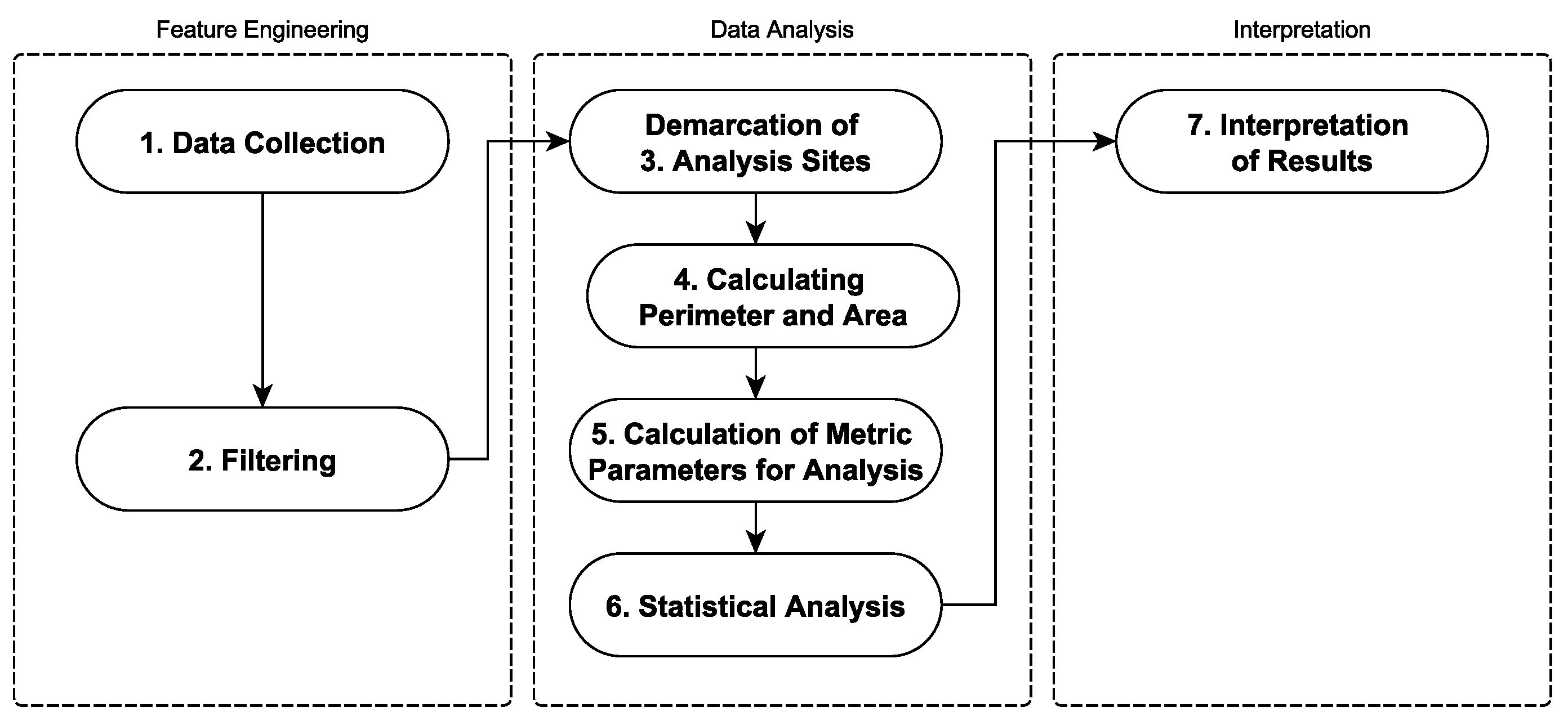
Figure 2.
Element distributions across clusters 2, 5, 6, and 7, plotted on a normalized exponential scale to emphasize variations in density and positioning.
Figure 2.
Element distributions across clusters 2, 5, 6, and 7, plotted on a normalized exponential scale to emphasize variations in density and positioning.
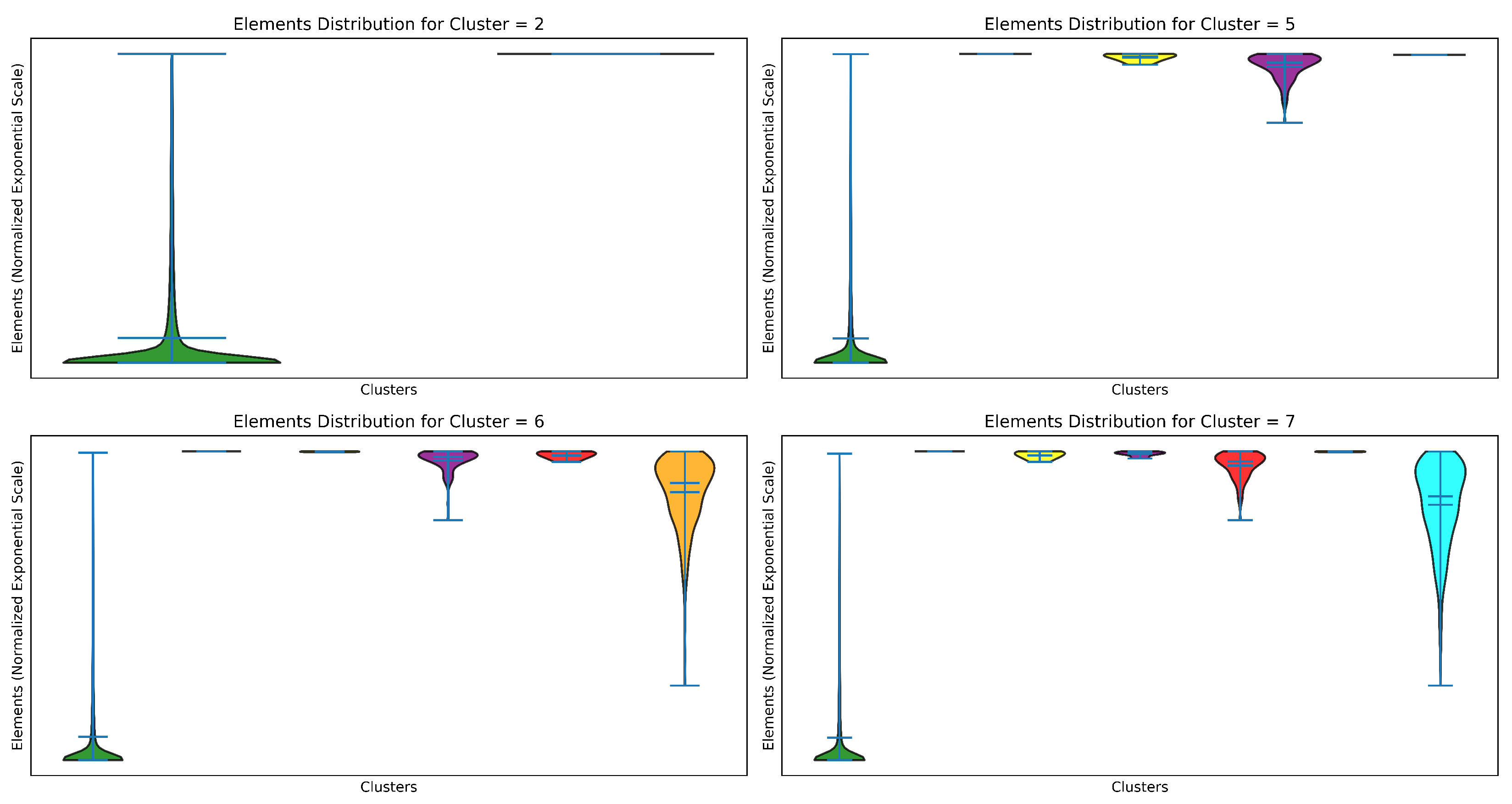
Figure 3.
Logarithmic histograms show the frequency distribution of area sizes. (a) Histogram for PPA area sizes, highlighting smaller regions with higher frequencies. (b) The histogram for LR area sizes shows a similar skewed distribution but over larger scales.
Figure 3.
Logarithmic histograms show the frequency distribution of area sizes. (a) Histogram for PPA area sizes, highlighting smaller regions with higher frequencies. (b) The histogram for LR area sizes shows a similar skewed distribution but over larger scales.
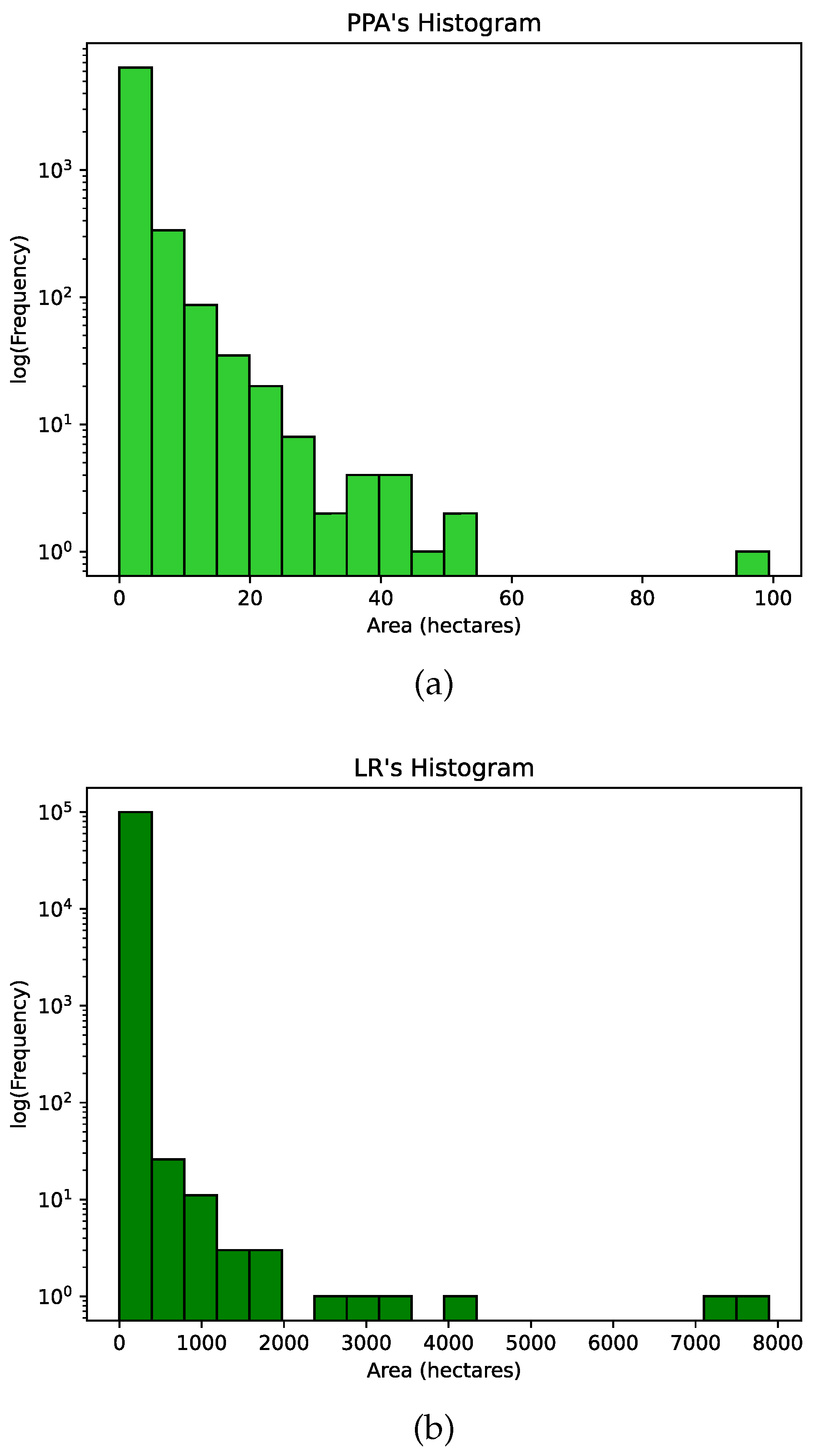
Figure 4.
Spatial distribution of highlighted areas in a region of Brazil. The Featured Area (red-dashed rectangle) is zoomed in to show specific locations of interest. Insets detail the highlighted areas: (A, B) PPA regions and (C, D) LR regions, demonstrating the spatial patterns and varying densities of the mapped regions.
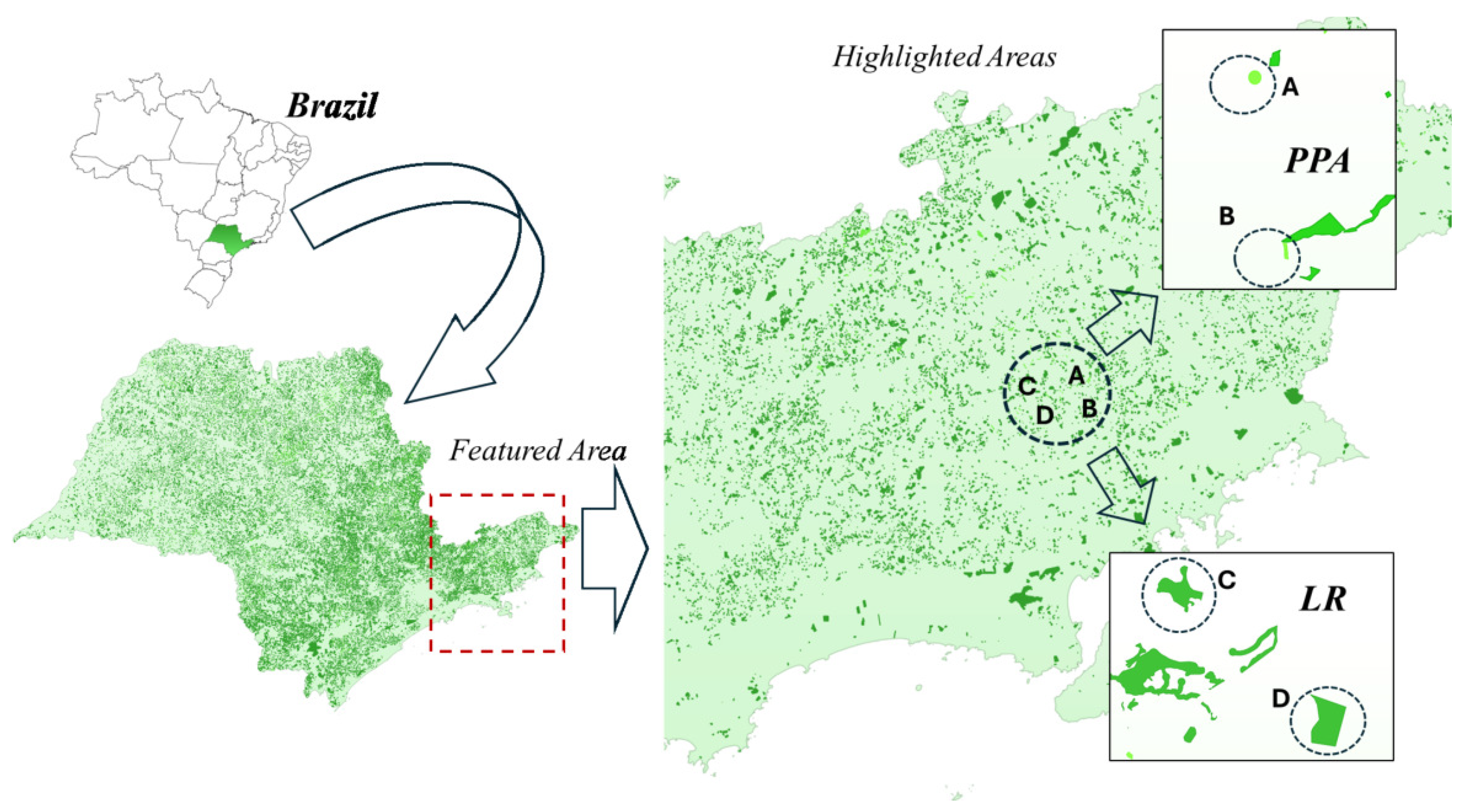
Figure 5.
Comparison of mean values for key metrics , , , across small, medium, and large fragments for PPA and LR datasets. The stacked bar plot highlights the relative contributions of fragment sizes to each metric, illustrating differences in interior compactness, edge factors, fractal dimensions, and compactness indices.
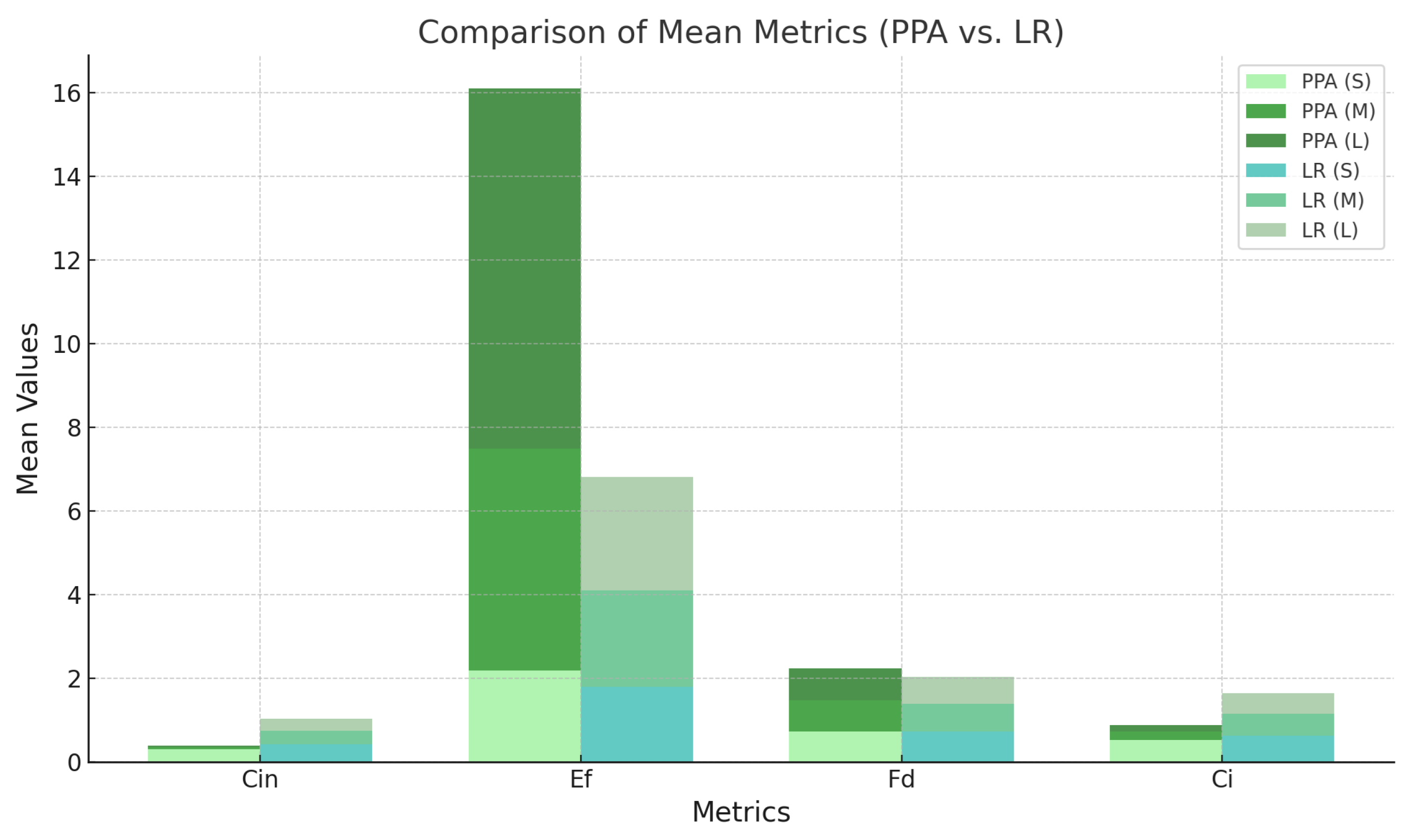
Figure 6.
Correlation Matrix: Highlighting Relationships Between Variables with Strength and Direction of Correlations. The matrix visually represents the pairwise correlation coefficients among features such as area, perimeter, radius, circle area, and geographic variables (latitude, longitude, height). Values range from (perfect negative correlation) to (perfect positive correlation), with a gradient color scale indicating the intensity of the relationships. Darker shades represent stronger correlations, while lighter shades indicate weaker or no correlation. Notable insights include a strong positive correlation between area and perimeter and a strong negative correlation between IC and FB.
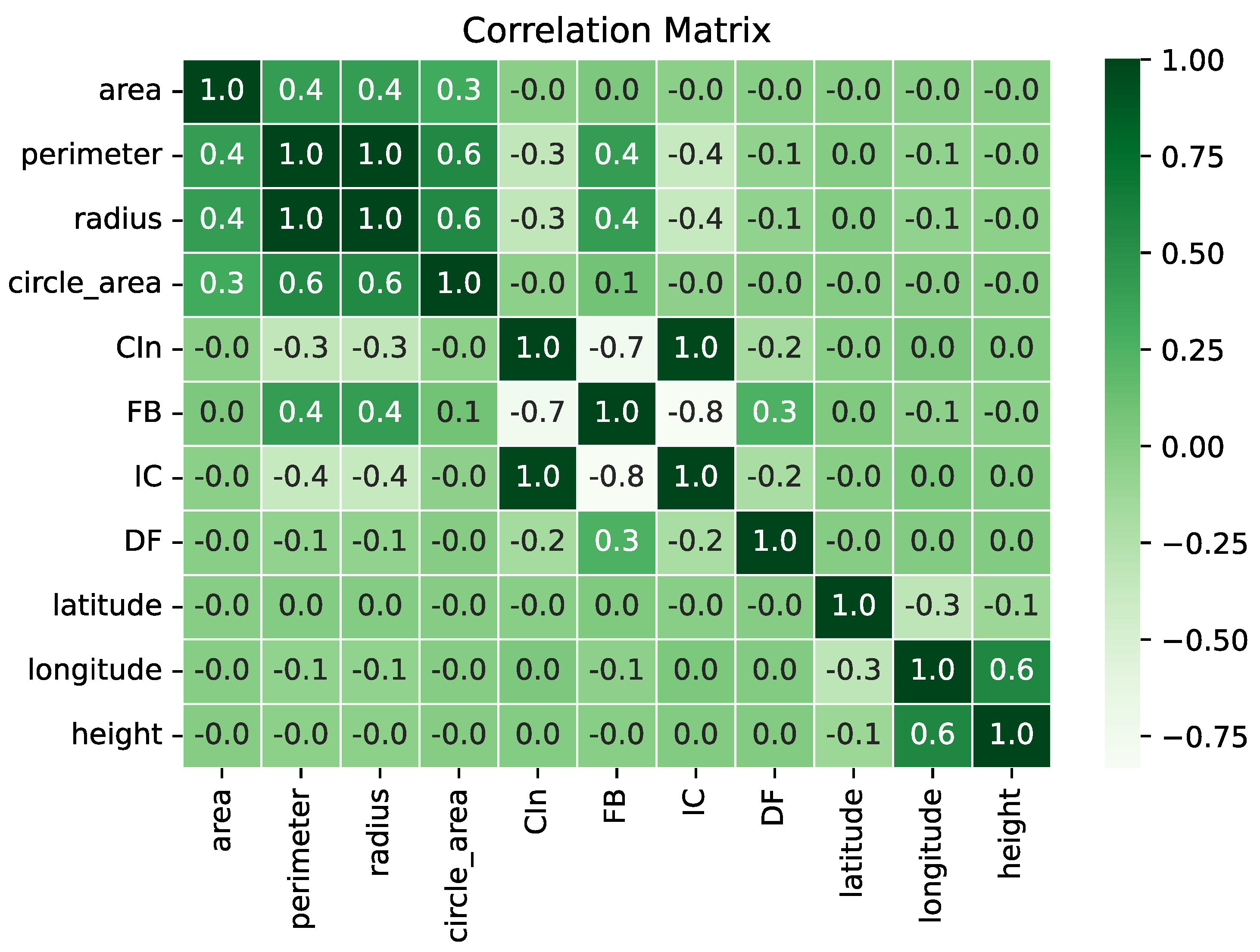
Figure 7.
Visualization of an irregularly shaped fragment with a low Circularity Index , illustrating its highly elongated and fragmented structure, which may contribute to increased edge effects and habitat vulnerability.
Figure 7.
Visualization of an irregularly shaped fragment with a low Circularity Index , illustrating its highly elongated and fragmented structure, which may contribute to increased edge effects and habitat vulnerability.
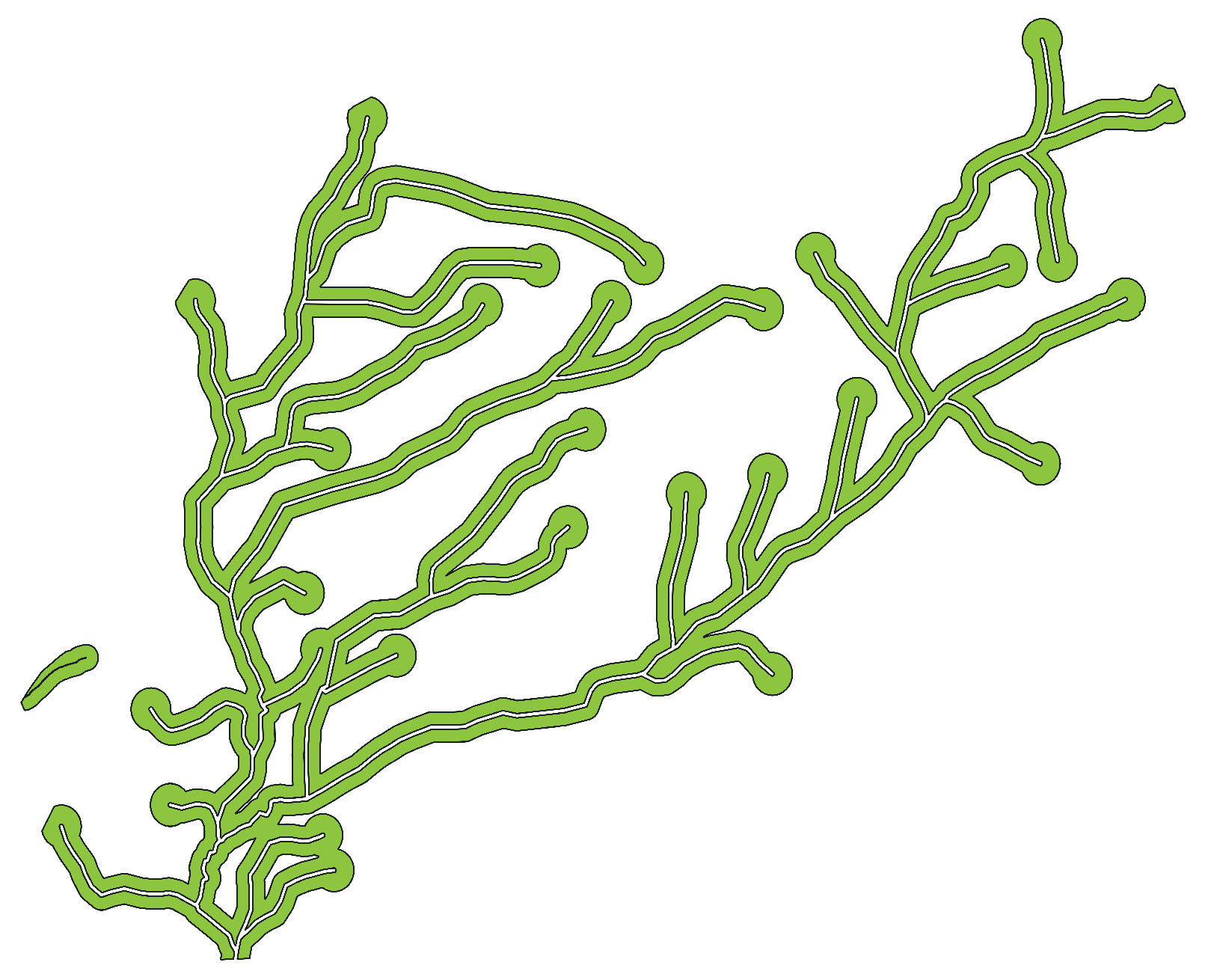
Figure 8.
Clusters visualized in 2D space using PCA with logarithmic scaling, highlighting the separation and distribution of data points across six distinct clusters.
Figure 8.
Clusters visualized in 2D space using PCA with logarithmic scaling, highlighting the separation and distribution of data points across six distinct clusters.
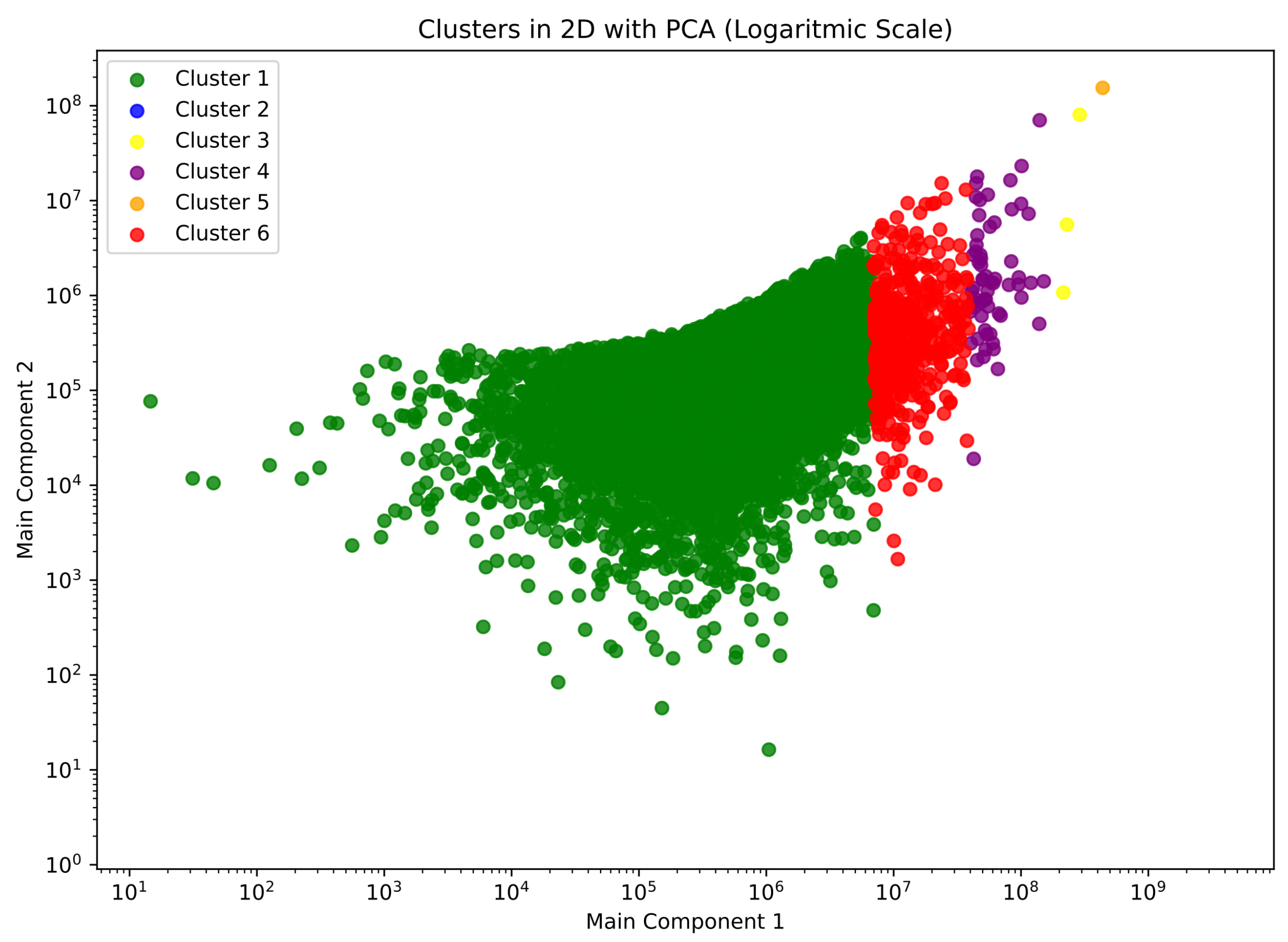
Table 1.
Metrics of Geospatial Form Indexes Used to Assess PPA and RL
| Metric | Purpose |
|---|---|
| Circular shapes minimize edge effects, reducing vulnerability to external influences (e.g., wind, temperature changes). Values near 1 indicate compact shapes, ideal for biodiversity conservation. Irregular shapes (e.g., elongated) have higher edge-to-interior ratios, increasing exposure to disturbances and species loss. | |
| Irregular edges are more vulnerable to disturbances. High values indicate irregular or fragmented edges, requiring targeted conservation strategies. | |
| Higher values indicate greater geometric complexity. Allows multi-scale spatial analysis of geospatial fragments, providing resilience and ecosystem dynamics. | |
| Compact areas exhibit less exposure to edge effects, promoting ecological resilience. Shapes closer to a circle are more efficient in protecting their interiors. |
The metrics presented are widely used in geospatial analysis to assess shape compactness, edge vulnerability, and spatial complexity. Proper interpretation can guide ecological management and conservation strategies.
Table 2.
Dataset Description
| Patch local | Quantity | Quantity (%) | Total area (ha) | Area % |
|---|---|---|---|---|
| PPA | 7,000 | 6.54 | 12,628 | 2.42 |
| LR | 100,000 | 93.46 | 508,504.5 | 97.58 |
| TOTAL | 107,000 | 100.00 | 521,132.5 | 100.00 |
Table 3.
Step-by-step Method Used to Determine Metric Parameters Using Satellite Images
| # | Step | Description |
|---|---|---|
| 1 | Data collection | The data is collected and separated from the relevant information from the shapefiles into a specific database. This step is necessary to validate information of interest and avoid errors in processing. |
| 2 | Filtering | Data filtering removes outliers, preventing contamination of the indicator parameter. |
| 3 | Demarcation of analysis sites | Filters are applied to select polygons of the Polygon type. Fragments are randomly chosen within the resulting sample, so there is no trend in the resulting data. |
| 4 | Calculating Perimeter and Area | GIS tools calculate the perimeter P and area A values for each fragment. (The software can provide these measurements with high precision). A centroid is also generated for each shape, storing its latitude and longitude coordinates so that it is possible to know the spatial location. The altitude of the area is obtained based on the centroid. |
| 5 | Calculation of metric parameters for analysis | With the perimeter and area data obtained, the indexes for each fragment are calculated, namely: circularity index (Cin), edge factor (Ef), fractal dimension (Fd), and compaction index (Ci), according to the metrics of the formula shown. |
| 6 | Statistical analysis | Statistical information about the data collection is calculated based on the measurements. The K-Means algorithm creates clusters to classify the data into specific data sets. |
| 7 | Interpretation of results | After calculating metrics for all fragments, the results are analyzed to identify patterns in the shape of the fragments and their relationship to geospatial factors such as connectivity, edge effects, and exposure to disturbances. |
Table 4.
Descriptive Statistics of the Distributive Property Areas of PPA and LR
| Type | Total Area (ha) | Mean | Median | SD | SE | Qty. |
|---|---|---|---|---|---|---|
| PPA | 12,628 | 1.82 | 0.86 | 3.39 | 0.04 | 7,000 |
| LR | 508,504 | 5.17 | 1.03 | 53.17 | 45.80 | 100,000 |
Note: SD = Standard Deviation; SE = Standard Error of the Mean.
Table 5.
Comparison of geometric and spatial metrics for Fragment A and Fragment B. Fragment A exhibits higher circularity and compactness, while Fragment B shows a more irregular shape, as reflected in its lower circularity index and higher boundary factor.
Table 5.
Comparison of geometric and spatial metrics for Fragment A and Fragment B. Fragment A exhibits higher circularity and compactness, while Fragment B shows a more irregular shape, as reflected in its lower circularity index and higher boundary factor.
| Fragment A (PPA) | Fragment B (PPA) |
|---|---|
| Total Area: 0.713 ha | Total Area: 0.29 ha |
| Perimeter: 300.22 meters | Perimeter: 298.17 meters |
| Circularity Index: 0.99447 | Circularity Index: 0.41267 |
| Edge Factor: 1.00277 | Edge Factor: 1.55665 |
| Fractal Dimension: 0.64294 | Fractal Dimension: 0.71406 |
| Compactness Index: 0.99721 | Compactness Index: 0.64239 |
 |
 |
Table 6.
Comparison of geometric and spatial metrics for Fragment A and Fragment B. Fragment A exhibits higher circularity and compactness, while Fragment B shows a more irregular shape, as reflected in its lower circularity index and higher boundary factor.
Table 6.
Comparison of geometric and spatial metrics for Fragment A and Fragment B. Fragment A exhibits higher circularity and compactness, while Fragment B shows a more irregular shape, as reflected in its lower circularity index and higher boundary factor.
| Fragment C (LR) | Fragment D (LR) |
|---|---|
| Total Area: 13.77 ha | Total Area: 20.67 ha |
| Perimeter: 3,055.27 meters | Perimeter: 2,096.17 meters |
| Circularity Index: 0.18541 | Circularity Index: 0.59089 |
| Edge Factor: 2.32233 | Edge Factor: 1.30090 |
| Fractal Dimension: 0.67816 | Fractal Dimension: 0.62489 |
| Compactness Index: 0.43060 | Compactness Index: 0.76869 |
 |
 |
Table 7.
Summary of Metrics Applied to PPA and LR
| Fragment | Type | Measured Factors | Calculated parameters | ||||
|---|---|---|---|---|---|---|---|
| Area (ha) | Perimeter (m) | ||||||
| A | PPA | 0.71 | 300.22 | 0.99447 | 1.00277 | 0.64294 | 0.99721 |
| B | PPA | 0.29 | 298.17 | 0.41267 | 0.64294 | 0.71406 | 0.64239 |
| C | LR | 13.77 | 3,055.27 | 0.18541 | 2.32233 | 0.67816 | 0.43060 |
| D | LR | 20.67 | 2,096.17 | 0.59089 | 1.30090 | 0.62489 | 0.76869 |
Table 8.
The Size Distribution of PPA Area Levels in of the Results
| Type | Area | Size (ha) | Quantity | % |
|---|---|---|---|---|
| PPA | S | X < 4.5 | 6,387 | 91.243 |
| PPA | M | 4.5 ≤ X < 20 | 571 | 8.157 |
| PPA | L | X ≥ 20 | 42 | 0.600 |
Table 9.
Descriptive Statistics of the Distributive Property Areas of PPA
| Measures | ||||||||||||
|---|---|---|---|---|---|---|---|---|---|---|---|---|
| S | M | L | S | M | L | S | M | L | S | M | L | |
| Mean | 0.310 | 0.057 | 0.028 | 2.185 | 5.316 | 8.598 | 0.724 | 0.754 | 0.765 | 0.524 | 0.215 | 0.143 |
| Median | 0.248 | 0.041 | 0.013 | 2.008 | 4.955 | 8.873 | 0.721 | 0.760 | 0.780 | 0.498 | 0.202 | 0.113 |
| Mode | 0.052 | 0.003 | 0.003 | 2.258 | 1.087 | 1.976 | 0.728 | 0.623 | 0.657 | 0.228 | 0.054 | 0.054 |
| Variance | 0.047 | 0.007 | 0.002 | 0.785 | 3.360 | 9.556 | 0.004 | 0.001 | 0.001 | 0.035 | 0.010 | 0.008 |
| Standard Deviation | 0.216 | 0.081 | 0.047 | 0.886 | 1.833 | 3.091 | 0.060 | 0.027 | 0.034 | 0.187 | 0.102 | 0.090 |
| Standard Error | 0.003 | 0.003 | 0.007 | 0.011 | 0.078 | 0.477 | 0.001 | 0.001 | 0.005 | 0.002 | 0.004 | 0.014 |
| Min | 0.002 | 0.003 | 0.003 | 1.002 | 1.087 | 1.976 | 0.639 | 0.623 | 0.657 | 0.045 | 0.054 | 0.054 |
| Max | 0.997 | 0.847 | 0.256 | 21.980 | 18.526 | 18.526 | 3.663 | 0.815 | 0.803 | 0.998 | 0.920 | 0.506 |
| Range | 0.995 | 0.844 | 0.253 | 20.978 | 17.440 | 16.550 | 3.024 | 0.192 | 0.146 | 0.953 | 0.866 | 0.452 |
| Dispersion | 1.073 | 5.362 | 3.608 | 3.119 | 1.364 | 0.191 | 24.495 | -2.261 | -1.816 | 0.467 | 3.212 | 2.577 |
| Kurtosis | 0.581 | 34.798 | 14.510 | 48.105 | 6.079 | 1.918 | 1.041 | 6.457 | 2.705 | -0.563 | 13.574 | 6.900 |
Table 10.
The Size Distribution of LR Area Levels in 100% of the Results
| Area | Trail bands | Size (ha) | Quantity | % |
|---|---|---|---|---|
| LR | S | X < 11 | 91,165 | 91.165 |
| LR | M | 11 ≤ X < 70 | 879 | 8.079 |
| LR | L | X ≥ 70 | 756 | 0.56 |
Table 11.
Descriptive Statistics of the Distributive Property Areas of LR
| Measure | ||||||||||||
|---|---|---|---|---|---|---|---|---|---|---|---|---|
| S | M | L | S | M | L | S | M | L | S | M | L | |
| Mean | 0.425 | 0.317 | 0.303 | 1.803 | 2.306 | 2.699 | 0.729 | 0.663 | 0.649 | 0.626 | 0.525 | 0.501 |
| Median | 0.416 | 0.264 | 0.263 | 1.550 | 1.946 | 1.950 | 0.696 | 0.658 | 0.638 | 0.645 | 0.514 | 0.513 |
| Mode | 0.016 | 0.290 | 0.002 | 1.053 | 1.857 | 1.058 | 0.632 | 0.656 | 0.588 | 0.126 | 0.539 | 0.047 |
| Variance | 0.047 | 0.048 | 0.052 | 0.698 | 1.343 | 3.638 | 0.099 | 0.001 | 0.002 | 0.033 | 0.041 | 0.051 |
| Standard Deviation | 0.218 | 0.220 | 0.229 | 0.835 | 1.159 | 1.907 | 0.315 | 0.036 | 0.040 | 0.001 | 0.002 | 0.008 |
| Standard Error | 0.001 | 0.002 | 0.008 | 0.003 | 0.013 | 0.069 | 0.001 | 0.000 | 0.001 | 0.065 | 0.091 | 0.047 |
| Min | 0.004 | 0.008 | 0.002 | 1.000 | 1.042 | 1.058 | 0.616 | 0.601 | 0.588 | 1.000 | 0.960 | 0.946 |
| Max | 0.999 | 0.921 | 0.894 | 15.427 | 11.025 | 21.453 | 20.960 | 0.807 | 0.782 | 0.935 | 0.869 | 0.899 |
| Range | 0.995 | 0.913 | 0.892 | 14.426 | 9.983 | 20.395 | 20.344 | 0.207 | 0.195 | -0.381 | 0.074 | -0.042 |
| Dispersion | 0.119 | 0.550 | 0.429 | 3.825 | 1.649 | 2.935 | 30.766 | 0.533 | 0.703 | 0.001 | 0.002 | 0.008 |
| Kurtosis | -1.014 | -0.884 | -1.098 | 27.999 | 3.632 | 16.579 | 1303.0 | -0.530 | -0.415 | -0.673 | -1.124 | -1.280 |
Disclaimer/Publisher’s Note: The statements, opinions and data contained in all publications are solely those of the individual author(s) and contributor(s) and not of MDPI and/or the editor(s). MDPI and/or the editor(s) disclaim responsibility for any injury to people or property resulting from any ideas, methods, instructions or products referred to in the content. |
© 2025 by the authors. Licensee MDPI, Basel, Switzerland. This article is an open access article distributed under the terms and conditions of the Creative Commons Attribution (CC BY) license (http://creativecommons.org/licenses/by/4.0/).
Copyright: This open access article is published under a Creative Commons CC BY 4.0 license, which permit the free download, distribution, and reuse, provided that the author and preprint are cited in any reuse.


