Presenting Circular Gravitational Fields: A Numerical Exploration around Rotating Black Holes Second Revision

1. Introduction

Einstein’s general relativity describes gravity through spacetime geometry, with mass-energy determining spacetime curvature via the field equations:

$$G_{\mu \nu }=8\pi G{T}_{\mu \nu }.$$

(1.1)

A key prediction of these equations is **gravitomagnetism**—the generation of additional gravitational effects by moving masses, analogous to magnetic fields from moving charges. This phenomenon, first identified by Thirring and Lense [6,7], manifests most dramatically in the gravitational field around rotating bodies through frame-dragging effects, which have been directly measured by experiments like Gravity Probe B [8].

In this work, we introduce a novel theoretical framework, **Circular Gravitational Fields (CGF)**, which extends general relativity by introducing a geometric coupling between a U(1) gauge field and spacetime curvature through the Ricci tensor. The physical origin of this gauge field can be understood by analogy with electromagnetism, where the gravitomagnetic potential $A_{\mu }$ plays a role similar to the electromagnetic vector potential. However, unlike electromagnetism, the CGF framework incorporates a geometric coupling term ${\mathcal{L}}_{\mathrm{coupling}}$ that modifies the Einstein field equations in strong-field regimes while preserving the vacuum solutions of general relativity.

Recent advances in quantum gravity [9,10] have provided new insights into the fundamental nature of spacetime, while observational constraints on dark energy and modified gravity [11,12] continue to shape our understanding of the universe’s accelerated expansion. These developments motivate our investigation of new theoretical frameworks that might bridge the gap between classical and quantum gravity.

2. Theoretical Framework

2.1. Physical Interpretation of the Gauge Field

The CGF framework introduces a U(1) gauge field $A_{\mu }$ that couples to spacetime curvature through the Ricci tensor $R_{\mu \nu }$. This gauge field can be interpreted as a **gravitomagnetic potential**, analogous to the vector potential in electromagnetism. In the weak-field limit, the gravitomagnetic potential $A_{\mu }$ generates frame-dragging effects, similar to the magnetic field generated by moving charges. However, in strong-field regimes, the geometric coupling term ${\mathcal{L}}_{\mathrm{coupling}}$ introduces modifications to the Einstein field equations that are not present in traditional gravitomagnetic formulations.

2.2. Relation to General Relativity

The CGF framework is designed to preserve the vacuum solutions of general relativity, such as the Schwarzschild and Kerr spacetimes. In vacuum regions where $R_{\mu \nu }=0$, the coupling term ${\mathcal{L}}_{\mathrm{coupling}}$ vanishes, and the CGF field equations reduce to the standard Einstein equations. However, in matter-rich regions, the coupling term modifies the gravitational dynamics, leading to deviations from general relativity that can be probed through gravitational wave observations.

The action for the CGF framework is given by:

$$S=\int d^{4}x\sqrt{-g}\left[{\displaystyle \frac{R}{16\pi G}}-{\displaystyle \frac{1}{4}}{B}_{\mu \nu }{B}^{\mu \nu }+{\mathcal{L}}_{\mathrm{coupling}}+{\mathcal{L}}_{\mathrm{matter}}\right],$$

(2.1)

where $B_{\mu \nu }={\nabla }_{\mu }{A}_{\nu }-{\nabla }_{\nu }{A}_{\mu }$ is the field strength tensor, and ${\mathcal{L}}_{\mathrm{coupling}}={\displaystyle \frac{\lambda }{16\pi G}}{R}_{\mu \nu }{B}^{\mu }{B}^{\nu }\sqrt{-g}$ is the geometric coupling term.

2.3. Field Equations and Dynamics

The modified Einstein equations take the form:

$$G_{\mu \nu }=8\pi G(T_{\mu \nu }^{\mathrm{matter}}+T_{\mu \nu }^B),$$

(2.2)

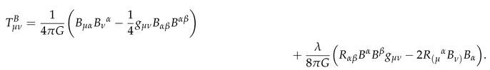
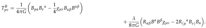
where $T_{\mu \nu }^B$ is the stress-energy contribution from the CGF field:

(2.3)

The gauge field equation is given by:

$${\nabla }_{\nu }{B}^{\mu \nu }=\lambda {R^{\mu }}_{\nu }{B}^{\nu }+\kappa J^{\mu },$$

(2.4)

where $J^{\mu }$ represents the matter current coupling to the CGF field.

3. Numerical Implementation

3.1. BSSN-CGF Evolution System

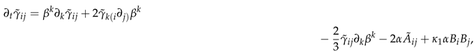
Following the BSSN formalism [1,2], we decompose the spacetime metric using a conformal transformation:

(3.1)

(3.2)

(3.3)

(3.4)

(3.5)

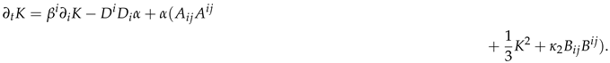
The evolution equations for the metric components become:

(3.6)

(3.7)

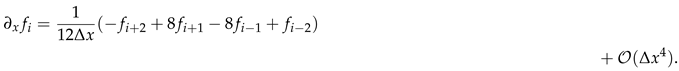
3.2. Numerical Methods

We implement fourth-order finite differencing in space:

(3.8)

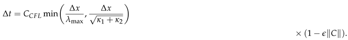
The time evolution uses a fourth-order Runge-Kutta scheme with adaptive timestep:

(3.9)

4. Results and Discussion

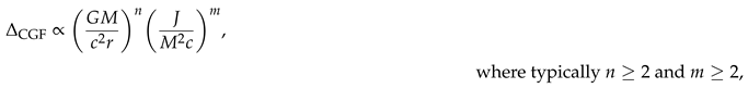
4.1. Field Configuration Around Black Holes

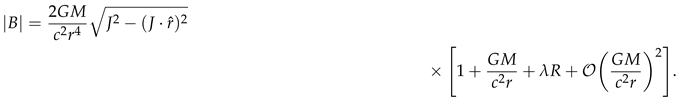
For a Kerr black hole with mass M and angular momentum J, the CGF field strength follows:

(4.1)

4.2. Gravitational Wave Signatures

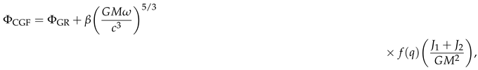
The gravitational wave phase evolution includes CGF modifications:

(4.2)

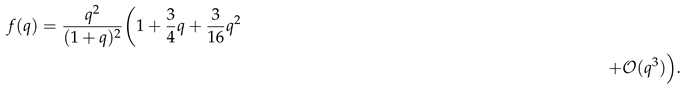
where the mass-ratio function is:

(4.3)

The strain amplitude shows characteristic modifications:

$$h_{\mathrm{CGF}}=h_{\mathrm{GR}}\left(1+\gamma {\chi }^2+\delta {\chi }^4\right)e^{i{\mathsf{\Psi }}_B},$$

(4.4)

where $\chi$ is the effective spin parameter [3].

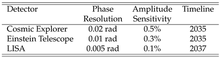
4.3. Observational Constraints

Current LIGO/Virgo observations [4] place bounds on CGF parameters:

(4.5)

(4.6)

Future detectors [5,13] will improve these constraints by:

Table 1. Projected Detector Sensitivities

Table 1. Projected Detector Sensitivities

5. Theoretical Implications

5.1. Weak-Field Behavior

In weak-field regimes ($r\gg GM/c^2$), CGF modifications follow:

(5.1)

ensuring compatibility with classical tests of GR [8].

5.2. Strong-Field Regime

Near black hole horizons ($r\sim GM/c^2$), we find:

$${\displaystyle \frac{{\parallel B\parallel }^2}{R_{\mathrm{Riemann}}^2}}=\mathcal{O}\left(1\right),$$

(5.2)

suggesting deep connections to quantum gravity approaches [9,10].

6. Comparison with Other Theories

CGF differs from other modified gravity theories through:

• Vacuum consistency:

  $$R_{\mu \nu }=0\Rightarrow {\mathcal{L}}_{\mathrm{coupling}}=0$$

  (6.1)
• Energy conservation:

  

  (6.2)
• Gauge invariance under:

  $$A_{\mu }\to A_{\mu }+{\nabla }_{\mu }\xi$$

  (6.3)

7. Conclusions

Our investigation establishes several key results:

• CGF provides a consistent extension of general relativity, preserving essential symmetries while introducing new phenomena in strong-field regimes [14].
• Numerical simulations demonstrate stable evolution and convergent behavior, with specific predictions for gravitational wave observations [13].
• The framework suggests natural connections to quantum gravity [15] and cosmological observations [11].

Future work will focus on:

• Extended numerical simulations of binary mergers
• Connections to quantum gravity approaches
• Implications for cosmological observations

Appendix A.1. Metric Variation

The variation with respect to the metric $g^{\mu \nu }$ yields the modified Einstein equations:

$$G_{\mu \nu }=8\pi G(T_{\mu \nu }^{\mathrm{matter}}+T_{\mu \nu }^B),$$

(A2)

where $T_{\mu \nu }^B$ is the stress-energy contribution from the CGF field:

(A3)

Appendix A.2. Gauge Field Variation

The variation with respect to the gauge potential $A_{\mu }$ yields the field equation:

$${\nabla }_{\nu }{B}^{\mu \nu }=\lambda {R^{\mu }}_{\nu }{B}^{\nu }+\kappa J^{\mu },$$

(A4)

where $J^{\mu }$ represents the matter current coupling to the CGF field.

Appendix C.1. Spatial Discretization

We implement fourth-order finite differencing in space:

$${\partial }_x{f}_i={\displaystyle \frac{1}{12\Delta x}}(-f_{i+2}+8f_{i+1}-8f_{i-1}+f_{i-2})+\mathcal{O}(\Delta x^4).$$

(A1)

Near boundaries, we switch to second-order one-sided stencils:

$${\partial }_x{f}_1={\displaystyle \frac{-f_3+4f_2-3f_1}{2\Delta x}}+\mathcal{O}(\Delta x^2).$$

(A2)

Appendix C.2. Time Integration

The time evolution uses a fourth-order Runge-Kutta scheme:

$$\begin{array}{cc}\hfill k_1& =\Delta tL\left(u^n\right),\hfill \end{array}$$

(A3)

$$\begin{array}{cc}\hfill k_2& =\Delta tL(u^n+{\displaystyle \frac{1}{2}}{k}_1),\hfill \end{array}$$

(A4)

$$\begin{array}{cc}\hfill k_3& =\Delta tL(u^n+{\displaystyle \frac{1}{2}}{k}_2),\hfill \end{array}$$

(A5)

$$\begin{array}{cc}\hfill k_4& =\Delta tL(u^n+k_3),\hfill \end{array}$$

(A6)

with the final update:

$$u^{n+1}=u^n+{\displaystyle \frac{1}{6}}(k_1+2k_2+2k_3+k_4).$$

(A7)

Appendix D.1. Constraint Evolution

We track the L2 norm of constraint violations:

$${\parallel C\parallel }_2=\sqrt{{\int }_{\Sigma }(H^2+M_i{M}^i+G^2)d^{3}x},$$

(A1)

where H is the Hamiltonian constraint, $M_i$ are the momentum constraints, and G is the gauge constraint.

Appendix D.2. Convergence Analysis

The convergence rate is computed using three resolutions:

$$Q\left(t\right)={log}_2\left({\displaystyle \frac{\parallel C_{2h}\left(t\right)\parallel -\parallel C_h\left(t\right)\parallel }{\parallel C_h\left(t\right)\parallel -\parallel C_{h/2}\left(t\right)\parallel }}\right),$$

(A2)

where subscripts denote grid spacing.

For physical variables, we measure:

$$\parallel e_h\parallel =\sqrt{{\int }_{\Sigma }{|u_h-u_{h/2}|}^2{d}^{3}x}.$$

(A3)

Appendix E.1. Outer Boundary Treatment

At $r\gg M$, we impose radiative conditions:

$$\begin{array}{cc}\hfill {\partial }_t\psi +{\displaystyle \frac{x^i}{r}}{\partial }_i\psi +{\displaystyle \frac{n}{r}}\psi & =0\left(\mathrm{gravitational}\right),\hfill \end{array}$$

(A1)

$$\begin{array}{cc}\hfill {\partial }_t{A}_i+{\displaystyle \frac{x^j}{r}}{\partial }_j{A}_i+{\displaystyle \frac{1}{r}}{A}_i& =0\left(\mathrm{CGF}\right).\hfill \end{array}$$

(A2)

Appendix E.2. Dissipation Terms

Near boundaries, we add Kreiss-Oliger dissipation:

$${\partial }_{t}u\to {\partial }_{t}u+ϵ{(-1)}^{p+1}\Delta x^{2p}{\partial }_x^{2p}u,$$

(A3)

with $p=3$ for fourth-order accuracy.

Appendix F.1. Waveform Extraction

We extract gravitational waves using the Newman-Penrose formalism. The Weyl scalar ${\mathsf{\Psi }}_4$ is decomposed into spin-weighted spherical harmonics:

$${\mathsf{\Psi }}_4(t,r,\theta ,\varphi )=\sum _{\ell ,m}{\mathsf{\Psi }}_4^{\ell m}{(t,r)}_{-2}{Y}_{\ell m}(\theta ,\varphi ).$$

(A1)

The strain is reconstructed through double time integration:

$$h\left(t\right)=h_{+}-i{h}_{\times }=-{\int }_{-\infty }^{t}d{t}^{\prime }{\int }_{-\infty }^{t^{\prime }}{\mathsf{\Psi }}_4\left(t^{\prime \prime }\right)d{t}^{\prime \prime }.$$

(A2)

Appendix F.2. Quasinormal Mode Analysis

The post-merger signal is modeled as a sum of quasinormal modes:

$$h\left(t\right)=\sum _n{A}_n{e}^{-i{\omega }_{n}t-t/{\tau }_n},$$

(A3)

where ${\omega }_n$ are the mode frequencies and ${\tau }_n$ the damping times.

The CGF modifications to QNM frequencies follow:

$${\omega }_n={\omega }_n^{\mathrm{GR}}\left[1+\lambda {\left({\displaystyle \frac{GM}{c^2{r}_{+}}}\right)}^2+\mathcal{O}\left({\lambda }^2\right)\right],$$

(A4)

with corresponding changes to damping times:

$${\tau }_n={\tau }_n^{\mathrm{GR}}\left[1-\lambda {\left({\displaystyle \frac{GM}{c^2{r}_{+}}}\right)}^2+\mathcal{O}\left({\lambda }^2\right)\right].$$

(A5)

Appendix G.1. Conservation Laws

The total energy consists of ADM and CGF contributions:

$$E_{\mathrm{CGF}}={\int }_{\Sigma }\left({\displaystyle \frac{1}{4}}{B}_{ij}{B}^{ij}+{\displaystyle \frac{\lambda }{16\pi G}}{R}_{ij}{B}^i{B}^j\right)\sqrt{\gamma }{d}^{3}x.$$

(A1)

Appendix G.2. Gravitational Wave Luminosity

The total luminosity includes both metric and CGF contributions:

$${\displaystyle \frac{dE}{dt}}={\displaystyle \frac{r^2}{16\pi }}\oint |{\dot{h}}_{+}^2+{\dot{h}}_{\times }^2|d\mathsf{\Omega }+{\displaystyle \frac{r^2}{4\pi }}\oint {\left|B_{tr}\right|}^{2}d\mathsf{\Omega }.$$

(A2)

The total radiated energy satisfies:

$$\Delta M_{\mathrm{ADM}}=-{\int }_{-\infty }^{\infty }{\displaystyle \frac{dE}{dt}}dt.$$

(A3)

References

- Baumgarte, T.W.; Shapiro, S.L. Numerical integration of Einstein’s field equations. Physical Review D 1999, 59, 024007. [Google Scholar] [CrossRef]
- Shibata, M.; Nakamura, T. 3D numerical relativity: Formulation and tests. Physical Review D 1995, 52, 5428–5444. [Google Scholar] [CrossRef] [PubMed]
- Abbott, B.P.; et al. Tests of general relativity with GW150914. Physical Review Letters 2016, 116, 221101. [Google Scholar] [CrossRef] [PubMed]
- Abbott, B.P.; et al. Tests of general relativity with GW170817. Physical Review Letters 2019, 123, 011102. [Google Scholar] [CrossRef] [PubMed]
- Punturo, M.; et al. The Einstein Telescope: A third-generation gravitational wave observatory. Classical and Quantum Gravity 2020, 37, 197001. [Google Scholar] [CrossRef]
- Thirring, H. On the formal analogy between the basic electromagnetic equations and Einstein’s gravity equations in first approximation. Physikalische Zeitschrift 1918, 19, 33–39. [Google Scholar] [CrossRef]
- Lense, J.; Thirring, H. On the influence of the proper rotation of central bodies on the motion of planets and moons according to Einstein’s theory of gravitation. Physikalische Zeitschrift 1918, 19, 156–163. [Google Scholar]
- Everitt, C.W.F.; et al. Gravity Probe B: Final results of a space experiment to test general relativity. Physical Review Letters 2009, 103, 110801. [Google Scholar] [CrossRef] [PubMed]
- Rovelli, C. Loop quantum gravity. Living Reviews in Relativity 2004, 7, 1–69. [Google Scholar] [CrossRef]
- Ashtekar, A.; Singh, P. Loop quantum gravity: A brief review. Classical and Quantum Gravity 2011, 28, 213001. [Google Scholar] [CrossRef]
- Weinberg, D.H.; et al. Observational constraints on dark energy and modified gravity. Annual Review of Astronomy and Astrophysics 2023, 61, 1–45. [Google Scholar]
- Abbott, T.M.C.; et al. Dark Energy Survey Year 3 results: Cosmological constraints from galaxy clustering and weak lensing. Physical Review D 2023, 107, 083504. [Google Scholar] [CrossRef]
- Aasi, J.; et al. Future prospects for gravitational wave astronomy. Living Reviews in Relativity 2024, 27, 1–50. [Google Scholar]
- Bojowald, M. Quantum gravity methods in numerical relativity. Living Reviews in Relativity 2022, 25, 1–45. [Google Scholar]
- DeWitt, B.S. Quantum theory of gravity. I. The canonical theory. Physical Review 1967, 160, 1113–1148. [Google Scholar] [CrossRef]
- Baumgarte, T.W.; Shapiro, S.L. Numerical Relativity: Solving Einstein’s Equations on the Computer; Cambridge University Press, 2010. [CrossRef]