Submitted:
09 January 2025
Posted:
13 January 2025
You are already at the latest version
Abstract
In this paper, we developed our own software that can analyze piano performance by utilizing short-time Fourier transform, non-negative matrix decomposition, and root mean square. In addition, for the reliability of the developed software, we provided results reflecting the characteristics of various performers and signal analysis. In conclusion, it shows the possibility that musical flow and waveform analysis can be visually interpreted in various ways. Based on this, we were also able to derive an additional approach suitable for designing the system to seamlessly connect hearing and vision.
Keywords:
short-time Fourier transform
; non-negative matrix decomposition
; music
; piano
1. Introduction
Sound wave analysis is necessary to understand music because it is not just a sensory pleasure, but also contains very complex structures and patterns in terms of science and technology. Through sound wave analysis, we can deeply understand the components of music, and through this, we can use them for music creation, learning, and research [1,2,3].
Acoustic analysis tools have evolved to enable humans to better understand and utilize sound. These tools started from simple auditory evaluation in the past and have evolved into advanced systems that utilize precise digital signal processing technology [4].
In the early stages of the development of acoustic analysis tools, subjective evaluation using human hearing was the main focus. Using an oscillograph or an analog spectrum analyzer, most of all mechanical devices could do was visually analyze the waveform or frequency of sound waves [5,6,7].
However, with the advent of the digital age, we began to analyze sound data using computers and software.
Fast Fourier Transform (FFT) has become a key technology in frequency domain analysis, and improved precision has made it possible to pinpoint the temporal and frequency characteristics of sound [8,9].
Recently, with the development of machine learning and AI-based analysis, technology is also being used to recognize patterns of sound, separate voice and instruments, and analyze emotions. Real-time sound analysis is possible through mobile devices and cloud computing, and thanks to 3D sound analysis, three-dimensional analysis is also possible by considering spatial sound information.Extending this to another application is expected to lead to infinite pioneering in a variety of fields, including healthcare (hearing testing), security (acoustic-based authentication), and environmental monitoring (noise measurement).
But there are also obvious limitations. First, the technical limitation is that analysis accuracy in complex environments is poor. It is difficult to extract or analyze specific sounds in noisy or resonant environments. In addition, it is difficult to process various sound sources, making it difficult to accurately separate sound sources with different characteristics such as musical instruments, human voices, and natural sounds [10]. Another limitation is the lack of versatility: there are many tools optimized for a particular domain, but no general-purpose system is built to handle all acoustic data.The biggest limitation is the gap between human hearing. Due to the difficulty in quantifying subjective sound quality assessments, it is difficult to fully quantify or replace a person’s subjective listening experience, and techniques to elaborately analyze human cognitive responses to sound (emotion, concentration, etc.) are still in their infancy [11].
Therefore, it is necessary to strengthen the technology to separate specific sound sources even in complex environments, and multimodal analysis should be developed to integrate various data such as video and text in addition to sound so that sound can be analyzed.
It also requires the development of models that better mimic the way the human hearing system works and acoustic calibration techniques tailored to individual hearing characteristics [12].
To sum up, acoustoassay tools are moving beyond just their role as technical tools to gain a deeper understanding of humans and their environment and provide a better experience. Future developments depend on integrating technology with human sensory and cognitive elements [13].
In this paper, we have developed a software that focuses on the quantification of subjective sound quality evaluation and present a method for analyzing various sound sources in various ways.
We also cognitively analyzed the performance of each of the three pianists (Younju Kim, Juhyun Ku, and Hyoen Park) for versatility evaluation and proof.
2. Necessity Needs for Analytical Tools
2.1. Understanding the Basic Components of Music
Music consists of physical elements such as amplitude, frequency, and temporal structure (rhythm). Sound wave analysis allows for quantitative measurement and understanding of these elements.
Frequency analysis makes it easier to check the pitch of a note and to understand the composition of chords and melodies. Time analysis can identify rhythm patterns and beat structures, and spectrum analysis can identify the unique tone (sound color) of an instrument [14].
2.2. Instruments and Timbre Analysis
Each instrument has its own sound (pitched tone), which comes from the ratio of its fundamental frequency to its background tone. Sound analysis visualizes these acoustic characteristics and helps to understand the differences between instruments.
For example, even at the same pitch as the violin and piano, the difference in tone is due to a combination of frequency components [15].
2.3. Understanding the Emotional Elements of Music
Music is used as a tool for expressing emotions, and certain frequencies, rhythms, and combinations induce emotional responses.
For example, slow rhythms and low frequencies are mainly used to induce sadness, and fast rhythms and high frequencies are used to induce joy.
Sound wave analysis can study these relationships to determine the correlation between emotions and music [16].
2.4. A Structural Analysis of Music
The structure of music is not just an arrangement of sounds, but includes complex patterns such as melody, chord, rhythm, and texture. Sound wave analysis allows us to visualize the structural elements of music.
For example, harmonic analysis can help you understand how chords and chords progression, and by analyzing the melody, you can check the pitch and rhythm pattern. Additionally, if multiple melodies are played simultaneously, you can understand the interaction of each melody [17].
2.5. Support for Music Production and Mixing
Sound wave analysis is essential for solving technical problems in the music production process.
You can adjust the sound volume by frequency band to balance the instruments and remove unwanted sound from recorded sound waves. Sound design also helps analyze and improve sound effects [18].
2.6. Music Learning and Research
Sound wave analysis provides music learners and researchers with tools to visually understand music theory.
2.7. Improved Listening Experience
Sound wave analysis can visually identify sound elements that are difficult to hear by the human ear (e.g., ultra-low, ultra-high) and improve the listening experience.For example, we can find hidden detailed sounds in music through spectrograms, and you can visually see the acoustic complexity of music.
The level of analysis and tools required may vary depending on the purpose of analyzing music, but for whatever reason sonic analysis is a powerful tool to explore the scientific and artistic nature of music beyond just listening [19].
3. Prior studies
3.1. A Way of Expressing Sound
There are many ways in which sound is expressed, but it is mainly explained by physical principles such as vibration, waves, and frequency. Sound is a pressure wave that is transmitted through air (or other medium) as an object vibrates. Let’s take a closer look at it.
Sound is usually produced by an object vibrating. For example, when a piano keyboard is pressed, the strings vibrate, and the vibrations are transmitted into the air to be recognized as sound. This vibration is caused by an object moving and compressing or expanding air particles.
And this sound is transmitted through a medium (air, water, metal, etc.). The particles of the medium vibrate, compress and expand to each other, and sound waves are transmitted. At this time, the important concepts are pressure waves and repetitive vibrations.
Compression is a phenomenon in which the particles of the medium get close to each other, and re-action is a phenomenon in which the particles of the medium get away, and the sound propagates by repeating these two processes, through which we hear the sound.
These sounds can be distinguished by many characteristics. Mainly, the following factors play an important role in defining sounds.
(1) Frequency
The frequency represents the number of vibrations of the sound.
At this time, the frequency is measured in Hertz (Hz). For example, 440 vibrations per second are 440 Hz.
The higher the frequency, the higher the pitch, and the lower the pitch, the lower the pitch. Human ears can usually hear sounds ranging from 20 Hz to 20,000 Hz.
(2) Amplitude
The amplitude represents the volume of the sound, the larger the amplitude, the louder the sound, and the smaller the amplitude, the smaller the sound.
Amplitude is an important determinant of the “strength” of sound waves. A larger amplitude makes the sound louder, and a smaller amplitude makes it sound weaker.
(3) Wavelength
The wavelength is the distance that a vibration in a cycle occupies in space.The longer the wavelength, the lower the frequency, and the shorter the frequency, the higher the frequency.
(4) Timbre (Timbre)
Timbre is a unique characteristic of sound, formed by combining various elements in addition to frequency and amplitude.
For example, the reason why the piano and violin make different sounds even if they play the same note is that each instrument has different tones.
As in this study, in order to analyze sound with software, sound must be digitally expressed, and when expressing sound digitally, the sound is converted into binary number and stored.
Digital sound samples analog signals at regular intervals, converts the sample values into numbers, and stores them, which are used to store and reproduce sounds on computers.
In summary, sound is essentially a physical vibration and a wave that propagates through a medium. There are two main ways of expressing this, analog and digital, and each method produces a variety of sounds by combining the frequency, amplitude, wavelength, and tone of sound.
3.2. Traditional Method of Sound Analysis
Frequency analysis is a method of identifying the characteristics of a sound by decomposing the frequency components of the sound. It mainly uses Fourier Transform techniques.
Fourier transform is a mathematical method of decomposing a complex waveform into several simple frequency components (sine waves). This transform allows us to know the different frequencies that sound contains.
These Fourier Series and Fourier Transform allow us to analyze sound waves in the frequency domain.
Secondly, spectral analysis is a visual representation of the frequency components obtained through Fourier transform. This analysis visually shows the frequency and intensity of sound.
A spectrogram is a graph that shows the change in frequency components over time, and can visually analyze how sound changes over time.
In addition, time analysis is a method of analyzing sound waveforms over time. This method can track changes in the amplitude of sound over time.
Analyzing the waveform analysis at this time allows you to determine the sound volume, temporal change, and occurrence of specific events.
The waveform is a linear representation of the temporal variation of an analog signal or digital signal, and amplitude and periodicity can be observed.
You can also track the volume change by analyzing the amplitude of a sound over time. For example, you can determine the beginning and end of a specific sound, or you can analyze the state of attenuation and amplification of the sound.
Further in waveform analysis, characteristic waveform characteristics can also be extracted, which is particularly important for classification or characterization of acoustic signals.
3.3. The Characteristics of Piano Sound
The piano is a system with a built-in hammer corresponding to each key, and when the key is pressed, the hammer knocks on the string to produce a sound. The length, thickness, and tension of the string, and the size and material of the hammer are the main factors that determine the tone of the piano. Each note is converted into sound through vibrations with specific frequencies.
Frequency is an important factor in determining the pitch of a note. Piano notes range from 20 Hz to 4,000 Hz. They range from the lowest note of the piano, A0 (27.5 Hz), to the highest note, C8 (4,186 Hz).
The pitch is directly related to the frequency, and the higher the frequency, the higher the pitch, and the lower the frequency, the lower the pitch.
The piano’s scale consists of 12 scales, separated by octaves. For example, the A4 is 440 Hz, and the A5 doubles its frequency to 880 Hz.
Tone is an element that makes sounds different even at the same frequency. In other words, it can be said to be the “unique color” of a sound.
The tone generated by the piano is largely determined by its structure of harmonics. Since the piano can produce non-sinusoidal waveform sounds, each note contains several harmonics in addition to the fundamental frequencies. This pattern of tone makes the piano’s tone unique.
For example, the mid-range of the piano has a soft and warm tone, the high-pitched range has clear and sharp characteristics, and the low-pitched range has deep and strong characteristics.
Dynamic is the intensity of a sound, or the volume of a sound. In a piano, the volume varies depending on the intensity of pressing the keyboard. The piano is an instrument that allows you to delicately control decremental and incremental dynamics.
For example, the piano (p) is a weak sound, and the forte (f) is a strong sound. In addition to this, medium-intensity expressions such as mezzoforte (mf) and mezzo piano (mp) are possible.
In addition, the sound of the piano depends on the temporal characteristics such as attack, duration, and attenuation.
Attack is a rapid change in the moment a note begins. The piano’s note begins very quickly, and the volume is determined when the hammer hits the string.
The piano’s attack is instantaneous and gives a faster reaction than other instruments. For example, the pitch on the piano pops out right away, and the other instruments, such as string or woodwind, can start more smoothly.
Duration is a characteristic of how long a sound lasts after it is played. The piano strings gradually decay when they make a sound, because the string’s vibration gets weaker and weaker due to friction with the air or other factors. The length, thickness, and tension of the strings affect the duration of the sound at this time. If you use a pedal, you can increase the duration of the sound, but when you press the damper pedal, the strings continue to ring without stopping the vibration, making the sound longer.
If you look at the waveform, the piano is an instrument that generates non-sine sound. This is a complex waveform, not a sine wave, and several frequency components are mixed to create a rich tone.
The sound waves on the piano are rich in harmonics, so they have various tones and rich characteristics. For example, more low-frequency components are included in the lower register, and high-frequency components are more prominent in the upper register.
The notes generated by the piano can be divided into low, medium, and high notes, each range having the following characteristics.
-Blow (A0 to C4): It contains deep, rich, and strong low-frequency components. For example, Blow C1 has a very low frequency of 32.7 Hz.
-Middle tones (C4 to C5): range similar to the human voice, which is the key range of the piano. The mid tones of the piano have a balanced sound and a warm tone.
-High note (C6 to C8): It has a sharp, clear sound, and a clearer sound is produced at a fast tempo or high note.
In conclusion, the characteristics of the sound produced by the piano are influenced by a combination of several factors, including frequency, tone, attack and duration, dynamic, and attenuation. The piano is an instrument with very rich and complex harmonics, and its sound is characterized by fast attacks and various dynamic controls. In addition, the tone is determined by the characteristics of the strings used and the material of the hammer, which makes the piano sound a unique and distinctive sound.
3.4. Characteristics of Classical Piano Music
Piano classical music usually includes classical and romantic music, and its style has characteristic elements in musical structure, dynamics, emotional expression, and technical techniques.
First, complex chords and colorful tones are important features in piano classical music. Since the piano can play multiple notes at the same time, it is excellent at expressing different chords.
The way chords are created is the synthesis of sound waves, which combine several frequency components to create more complex and rich notes. In this process, each note has its own harmonics, which provides a touching and colorful tone to the music.
The second feature is that it delicately controls the dynamics. It can express dramatic changes and subtle emotions by crossing the piano(p) and the forte(f). It also expresses the rhythm and melody by using various technical techniques such as precise rhythms and arpeggios, trills, and scales.
These techniques require fast and repetitive vibrations, resulting in more complicated waveform fluctuations.
Lastly, classical piano music focuses on expressing emotional depth, and deals with epic development and emotional flow. The music delicately utilizes the dynamics and rhythm in expressing dramatic contrast or emotional height.
When viewed from the perspective of a scientific wave, the notes of classical piano music are not just sine waves but complex non-sinusoidal waveforms. Because of this, the piano’s sound includes harmonics, making it richer and more colorful in tone. This sonic quality is very important in classical music.
(1) Complex waveform structure
The waveform consists of a fundamental frequency and multiple overtones. For example, the piano’s sound vibrates according to its harmonic series, which means that in addition to the fundamental frequency, the background sounds such as 2x frequency, 3x frequency, and 4x frequency are also present.
Piano tones have frequencies higher than the basic notes, and they enhance or distort the characteristics of the basic notes. The tone of a piano is formed by the way these tones are nonlinearly combined.
For example, there are many and strong tones at lower notes, and relatively few and microscopic tones at higher notes.
(2) Quick attack and sudden waveform changes
In a piano, notes begin quickly, which is a part called an attack. The moment a note begins, the waveform undergoes a drastic change.
For example, the sound pressure on a piano rise very quickly as soon as the hammer hits the string, and then it attenuates rapidly. This causes a drastic change in the waveform.
The attack part is very short, producing an abnormal waveform indicating a spike with a fast frequency change. The waveform at this moment takes the form of a sharp peak and then a quick decrease in amplitude.
(3) Nonlinearity
The sound of classical piano music has nonlinear characteristics, forming unexpected waveforms through multiple nonlinear interactions, even at the same frequency.
For example, the moment a hammer hits a string, complex nonlinear oscillations can occur depending on the hammer’s mass, speed, and string tension. This results in a mixed waveform in addition to the fundamental frequency, which forms its own tone.
To sum up, the characteristics of piano classical music are very complex and colorful, ranging from its musical composition to the physical characteristics of the sound. Musically, it is characterized by complex chords and various dynamics, and it deals with emotional expression as important. These musical characteristics are physically revealed through the wave peculiarities of sound—complex waveforms, fast attacks, dynamic frequency changes, etc., and the singularity is well represented by the piano’s tonal structure and nonlinear waves. The sound waves of the piano are very rich and complex, which contribute to expressing the emotional depth and emotion that classical music is trying to convey well.
4. Method
4.1. Mathematical Techniques
4.1.1. Short-time Fourier Transform (STFT)
For a given signal x(t), the short-time fourier transform (STFT) is defined as follows:
Here, is time domain signal to analyze, while defined window function depending on .
The is called the window function, and it is used to extract only certain sections of the signal. Typical window functions include Hamming, Hanning, and Gaussian windows.
The shorter the length of the window function, the higher the time resolution, and the longer the frequency resolution.
The sliding window analyzes the signal by sliding the over time t.
After these processes, the results of STFT are given as complex numbers, amplitude represents the strength of the frequency component, and phase represents the phase of the frequency component.
In this case, the information provided in the form of a plural number includes two. The first is the intensity of the frequency expressed in the , and the second is the phase information of the frequency component expressed in the .
However, when actually analyzing a signal on the computer, the signal is discrete, so it is calculated by discretizing the STFT for continuous signals. For discrete signal x[n], the STFT is defined as follows:
where x[n] denotes the discrete signal, and is the window function applied in the time m.
Since N represents the length of the window or the size of the FFT, the frequency resolution determination is determined by N.
4.1.2. Autocorrelation
Autocorrelation is an important tool for analyzing the self-similarity of signals, measuring how repetitive or periodic they are over time.
The autocorrelation function of the continuous signal is defined as follows:
Autocorrelation functions can be applied in many ways in sonic analysis, first of all they are excellent for periodicity analysis.
For example, an automatic correlation function in which a signal is repeated can estimate the fundamental frequency from a voice signal.
It is also used to distinguish noise from useful components in signals. Noise is generally less correlated in time, while useful signals are highly correlated.
And we can also measure the signal energy mathematically.
Finally, it can be used to calculate the period (e.g., pitch) of a speech signal, or to detect a rhythm in a music signal.
Autocorrelation functions are closely related to Fourier transforms. In particular, according to the Wiener-Hinchin theorem:
In other words, the autocorrelation function of the signal pairs the size square of the Fourier transform of the signal with the Fourier transform .
This allows us to quickly compute the automatic correlation function via FFT.
The automatic correlation function is a very important tool in signal analysis and is used for a variety of purposes, including periodicity detection, noise cancellation, and energy calculation. For discrete signals, it can be calculated quickly using FFT and has a wide range of applications such as acoustic analysis, speech recognition, and bio-signal analysis
4.1.3. Non-Negative Matrix Factorization (NMF)
Non-negative matrix factorization (NMF) is a technique that decomposes a non-negative matrix into two non-negative matrices, and is used in various fields such as data analysis, dimensionality reduction, signal processing, and text mining. In this paper, we will explain this mathematically and provide intuition.
The NMF is based on the process of solving the following optimization problems:
The Frobenius norm represents the square of the Euclidean distance between the matrix X and .
NMF optimization is classified as a nonlinear optimization problem due to non-negative constraints. To address this, the following update method is used:
At this point, it ends when the convergence condition (e.g., the change in the Frobenius norm is below the threshold), and at each stage, it solves the least-squares problem with non-negative constraints to maintain the non-negative constraints.
NMF is a simple yet powerful matrix decomposition technique that is very useful for extracting patterns in data and interpreting hidden structures. However, it can be effectively utilized only when you understand the limitations and characteristics of NMF and set the appropriate parameters for the data.
4.2. Physical Tools
In this paper, we differentiated and coded the acoustic signal analysis tool by providing a user interface. The tool works modular, allowing users to blend and match different tools to tailor their interfaces and features to specific analysis requirements.
The key idea here is the analysis chain. We interconnect the signal itself or the signal analysis results to different windows to form a functional block sequence. It includes file input, data collection modules, FFT analysis, measuring instruments, etc.
There is only one segment of the signal needed to visually represent a musical signal. Efficient physical tools were used to effectively imitate real-time signal analysis using pre-recorded offline signals.
The sequence of all values is “signal” at this time. The concept of “signal” includes an array of all X/Y values, including audio signals, spectra, or other data representations. This broad definition means that all sequences are attributed to the sampling rate, which can also be applied to data not derived from digital sampling of analog signals. For example, the “sampling rate” of the FFT analysis results is determined by the number of bins (values) per unit of frequency (Hz) on the X-axis.
This framework enables a flexible analysis approach, such as performing FFT on the results of previous FFTs. The biggest advantage of this work is that there are no restrictions on analytical exploration. I would like to compare and analyze classical piano music while pioneering a unique methodology to achieve the desired insights.
Filtering is the process of removing or changing certain frequency components from a signal. As shown in Figure 1, our software simply defines the segment of the frequency to be removed or the segment you want to leave on the signal, and applies the filter to the signal. This allows us to create band-blocking, band-passing, high-pass, and low-pass filters.
Figure 2 shows a Python code that calculates the STFT of a 440Hz sine wave and visualizes it as a spectrogram.
Using this, it is possible to convert the signal without going through complicated calculations every time. Furthermore, it is easy to see the changes in the signal at a glance because it shows the graph consisting of spectrograms.
The code in Figure 3 generates a sine wave of 5 Hz and calculates the automatic correlation function of the signal using np.correlate. The visualization of the result is then plotted according to the lag.
When implementing NMF in Python as shown in Figure 4, the Sklearn library makes it easy to handle. In addition, implementing NMF with Python can benefit from productivity, scalability, learning opportunities, community support, and more. In particular, library support allows it to be used at various levels, from basic use to advanced tuning.
4.3. The Specifications of a Piano
The piano used for the performance and recording was the Yamaha Grand Piano GC1, which was produced in Japan. There were a total of 88 keys, a soft pedal (left), a Sostenuto pedal (center), and a damper pedal (right). The top lid was open in the recording environment.
The depth of the grand piano varies depending on the model, but it usually ranges from 151 cm to 188 cm.
For the grand piano used in this study, it should be noted that the total length from the keyboard to the longest string end is 161 cm, therefore the actual sound and the recorded sound may differ if no sinusoidal waves are made at that length.
4.4. Characteristics of Performed Music and Performers Characteristics
4.4.1. Twinkle, Twinkle, Little Star
This is part of Mozart Variations (12) on ‘Ah, vous dirai-je, Maman' in C major, K265. However, it is more familiar with the beginning of the song as ‘Twinkle, Twinkle, Little Star’. twinkling little star.
The theme is a folk melody consisting of 12 simple and simple bars.
It is composed in C major and features a clear and clear sound pattern.
4.4.2. Gavotte Composed by Cornelius Gurlitt
In this paper, we chose Gavotte composed by Cornelius Gurlitt because it is a specific song that can show the connection and disconnection of notes, and changes in articulation, a playing technique that represents legato and staccato, due to its relatively fast rhythm. It also has the advantage of being able to clearly express the visual through the waveform graph because the phrase section on the score is clear.
A total of five notes are connected to the regato until the first note of the next bar, followed by two staccato notes. If we look closely at this part, we can distinguish the waveform difference between the regato and staccato methods.
There’s also a part that gradually becomes a crescendo from the 9th bar to the 12th bar, and from the 13th bar to the 16th bar, we can even look at the volume in a single piece because it’s played quietly with the right hand only without the left hand.
4.4.3. Rachmaninoff Piano Concerto No. 2 in c Minor, Op. 18
In the case of the first seven bars, the two-handed chord that is pressed at the same time and the left-handed bass F alternate. In addition, since the right-handed inner part changes with each bar, it is easy to observe the change of sound waves with right-handed chords.
The volume of the sound is also gradually increasing from pp to ff, so you can see if the “feel of something coming from a distance” is also expressed on the graph when drawn in a waveform.
4.4.3. Characteristics of Performers
(1) Younju Kim, Female
166cm, 54kg, hand size: From the first note of Do to the next octave Mi.
She is characterized by having relatively long arms and is a performer with good movement. However, instead of having a large arm movement, the force cannot be transmitted quickly to the fingertips, making it difficult to perform strong strokes. The sound resonates well, but the amplitude is not large.
(2) Juhyun Ku, Female
163.5cm, 60kg, hand size: From the first note of Do to the next octave Mi.
The weight of the arms is heavier and the fingertips are harder than other pianists. There is less movement of the arms and the fingertips are attached to the piano to control the speed. It is characterized by less movement of the arms.
(3) Hyoeun Park, Female
161cm, 47kg, hand size: From the first note of Do to the next octave Re.
The weight of the arms is light and the movement is fast. She is one of the musicians who produce accurate sounds. When playing the piano, the movement is big, but the time when the hands are attached to the piano keys is short.
(4) Eunsung Jekal, Female
158, 42kg, beginner, who is learning from Younju Kim, hand size: From the first note of Do to the next octave Do.
Unlike other pianists, he recorded on the Kawai Digital Piano. He has been learning for about a year, so he has no movement in his arms and is very weak in other health compared to professional pianists.
5. Results
5.1. Magnitude of Sounds
Root Mean Square (RMS) represents the average energy of a signal and is the basic method for quantitative comparison of sound magnitudes as shown in Figure 5.
In this paper, two recorded files were imported into the software and calculated as the rms function of MATLAB.
Afterwards, we measured the Loudness Units Full Scale (LUFS). LUFS is an international standard that measures the loudness of sounds based on the volume felt by the human ear.
The LUFS values of the two performances were compared using the Loudness Normalization function, and it is generally considered that the lower the LUFS value, the higher the volume. That is, the size increases as it approaches zero.
Finally, we analyzed decibels (dB), and we gave it as Figure 6. Decibels compare the loudness based on the peak amplitude or average amplitude of the signal.
In this paper, the Peak Level and Average Level were measured using their own software, and the Peak Amplitude was calculated using MATLAB’s max (abs(signal).
Performer Jekal:
RMS: -20.5dB
LUFS: -15 LUFS
Dynamic range: 10 dB
Performer Ku:
RMS: -18.2dB
LUFS: -12 LUFS
Dynamic range: 14 dB
In conclusion, Ku makes an overall louder sound, and the dynamic range is also wider, showing that it is more expressive.
5.2. Velocity
By differentiating the waveform graph, you can get information that represents the rate of change of the signal. This rate of change can be interpreted as speed, which varies depending on the physical or mathematical properties of the signal. For acoustic signals, differentiation is useful for analyzing the rate of amplitude change or for deeply understanding the characteristics of the signal.
1st differential expressed as
2nd differential expressed as
Here, if it is calculated as a discrete signal instead of a continuous signal, it may be approximated as follows:
Figure 7 shows the change in speed by differentiating the waveform. Comparing (a) and (b) in the boxed sections, you can see that the change in (b) is more rapid. In other words, (b) the performer hits one note while playing the piano and then moves on to the next note compared to (a). This may have been due to the performer’s movement or body shape.
5.3. Touch Intensity
Figure 8.
Piano keyboard touch strength of (a)Jekal and (b)Park.
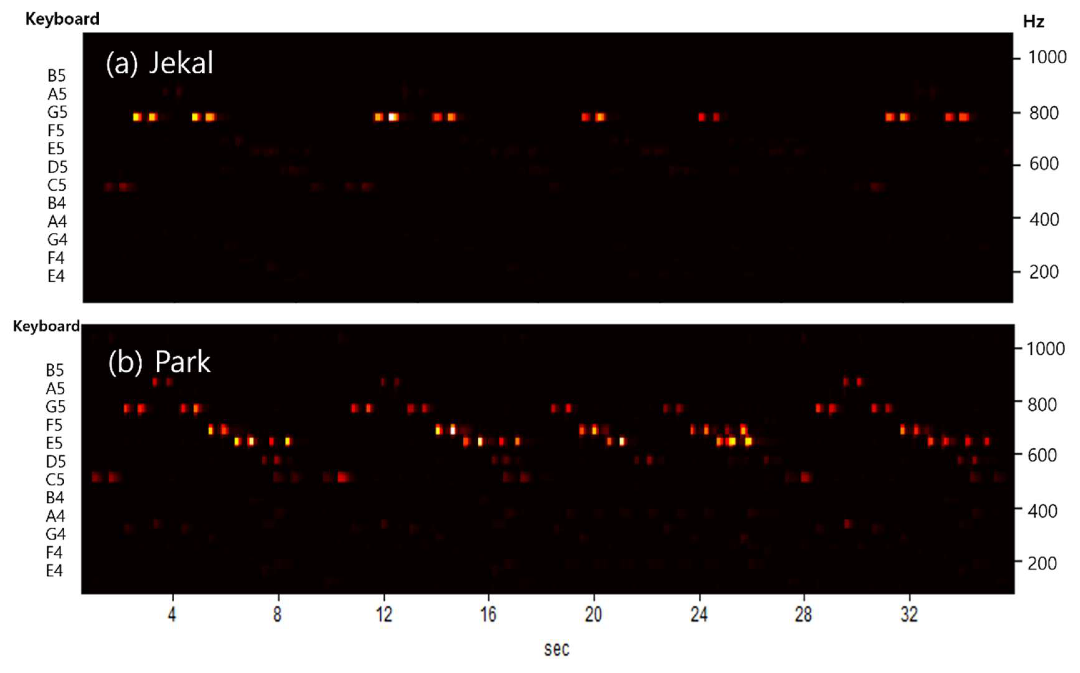
To mathematically analyze the strength (touch strength) of pressing the keys when playing the piano, you need to obtain and analyze data related to the force on the keys through acoustic signals or physical sensors. This can be represented by the amplitude of an acoustic signal, or the physical movement of the keys.
In this paper, amplitude-based analysis was utilized.
This is because the amplitude of the generated acoustic signal increases when the keyboard is pressed hard, so the intensity can be estimated by analyzing the amplitude.
For this purpose, the recorded acoustic signal was imported into its own analysis software, and the average amplitude was measured by calculating the RMS value of the signal.
The RMS is calculated as follows:
Here, expresses value of sample signal and denotes number of samples.
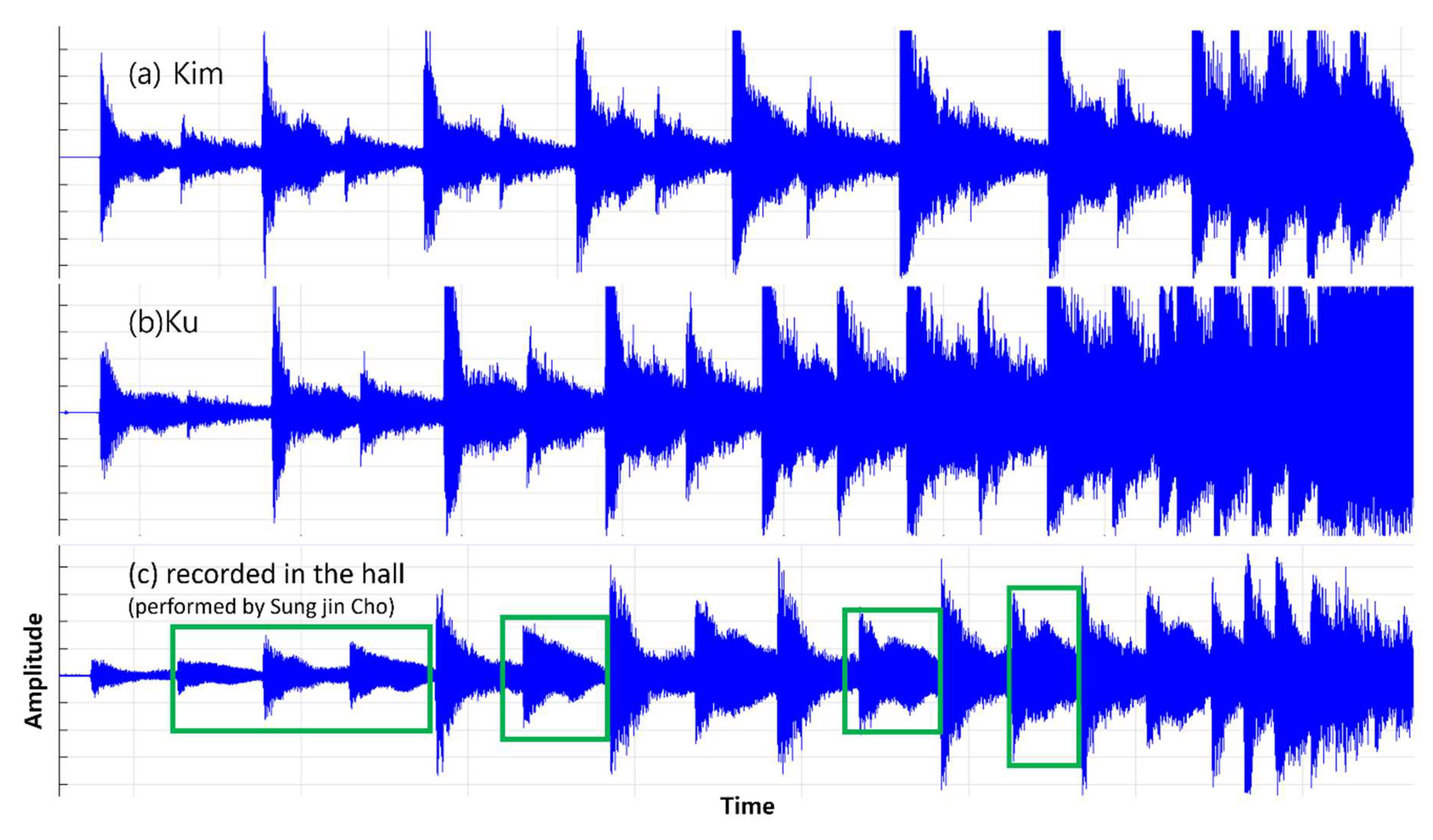
5.4. Music Flow
Gavotte composed by Cornelius Gurlit, expressed in the form of sound waves in Figure 9, can be largely divided into six parts. Section 1 and Section 2, and Section 5 and Section 6 are all played with the same note and rhythm. However, in Section 4, it can be seen that the sudden sound becomes smaller, and the difference between the three pianists can be seen more clearly here. The note played by Kim grows and decreases again, the note of the beat becomes louder and louder, and the note of the sphere becomes smaller and smaller. In the case of part 5 as well, Kim starts with a loud sound following section 4 and Park starts with a small sound before playing louder and louder.
In fact, it is often difficult to hear the change in detail when listening to fast songs such as Gavotte.
However, the software used in this study shows changes in the overall structure and musical image of the song well through the waveform graph.
Graph theory was used in this paper because it can be very useful in structural and relational analysis of piano music, and the results are shown in Figure 10.
First, the graph consists of node set and edge set , so it is expressed as .
Music has a direction, so we need a graph that considers the direction here, and the in-degree is expressed as
The out-degree is expressed as
and the sum of entry and exit orders for all nodes is expressed as
Entropy of graph denoted as
where .
In this way, graph theory can be used to create a key tool for analyzing music or solving problems that arise during the practice process.
6. Discussion
In this work, we explore ways to improve the smooth connection of visual and auditory flows through waveform analysis of music.
The sound was analyzed using mathematical techniques such as Short-Time Fourier Transform (STFT), Non-Negative Matrix Factorization (NMF), and Root Mean Square (RMS), and the analysis results reflecting the characteristics of various performers were presented.
Analyzing sound in this way allows various applications such as emotional expression, structural analysis, understanding differences in musical instrument tones, and supporting music production.
The sound volume analysis compared the size of the performance and the dynamic range through the analysis of the performer’s RMS, LUFS, and dB.
For velocity analysis, the rate of change of the signal and the difference in the movement of the performer were evaluated through the first and second derivatives of the waveform.
As for the touch intensity, the intensity of the keyboard touch was estimated by RMS, and the expressive power of the player was compared.
In addition, in the flow of music, the structural change of the song was visualized as a waveform graph to clearly confirm the difference in the interpretation of the performer.
7. Future Works
7.1. Overcome the Difference Between Soundproof Room and Hall
Figure 11.
- Improved visual-audible connection smoothness
Music waveforms can naturally have irregular, sharp shapes. To visualize them seamlessly, the signals need to be processed smoothly.
Low-pass Filter can be utilized for smoothing the signal, which reduces the high frequency component (noise) and softens the waveform.
In addition, Spline Interpolation creates curves that seamlessly connect data points, enabling smoother waveform representations.
There’s another way to enhance visual synchronization.
It reinforces visual effects, which align with auditory perception, by emphasizing features such as music’s rhythm, tempo, and range. For example, you might consider extracting the music’s rhythm through beat detection algorithms to synchronize visual “beat” or change the color according to frequency band or amplitude.
APPENDIX: Musical Terminology
1. The three elements of music
(1) chords(harmony): a combination of three or more notes
(2) melody: a combination of pitch and rhythm
(3) rhythm: the placement of sounds in time
2. The piano technique :
(1) arpeggio: a type of broken chord in which the notes that compose a chord are individually sounded in a progressive rising or descending order
(2) trill: a rapid alternation between two adjacent notes
(3) legato: technique and notation that indicates notes should be played smoothly and connected
(4) staccato: a style of playing music where notes are short, detached, and played briskly, with a small rest between each note
3. Dynamic marks :
(1) piano(p): soft sound
(2) forte(f): loud sound
(3) mezzo piano(mp): medium softness
(4) mezzo forte(mf): medium loud
(5) pianissimo(pp): softer than piano(p)
(6) fortissimo(ff): louder than forte(f)
(7) crescendo(cresc.): a gradual increase in loudness
4. Etc.
(1) tone: steady periodic sound
(2) pedal: foot-operated levers that change the sound of a piano by altering the strings or the hammer mechanism.
- Damper pedal: This pedal removes the dampers from the strings, allowing the notes to ring out longer.
-Sostenuto pedal: This holds notes that are already being played.
-Soft pedal: It is also known as the una corda pedal, this pedal shifts the hammer mechanism to the right, so the hammer only hits two of the three strings.
(3) harmonic: characterized by musical harmony
(4) scale: a series of notes arranged in order of pitch
(5) octave: the interval between two musical notes that have a frequency ratio of 2:1
(6) tempo: the speed at which a passage of music is played
References
- D. Arfib. Digital synthesis of complex spectra by means of multiplication of nonlinear distorted sine waves. Journal of the Audio Engineering Society 1979, 27, 757–768. [Google Scholar]
- B. Bank. Nonlinear interaction in the digital waveguide with the application to piano sound synthesis. In Proceedings of the International Computer Music Conference, pages 54–57, Berlin, Germany, September 2000a.
- B. Bank and V. Välimäki. Robust loss filter design for digital waveguide synthesis. IEEE Signal Processing Letters 2003, 10, 18–20. [Google Scholar] [CrossRef]
- J. Bensa, S. Bilbao, R. Kronland-Martinet, and J. O. Smith. The simulation of piano string vibration: From physical models to finite difference schemes and digital waveguides. Journal of the Acoustical Society of America 2003, 114, 1095–1107. [Google Scholar] [CrossRef] [PubMed]
- J. Berthaut, M. N. Ichchou, and L. Jézéquel. Piano soundboard: Structural behaviour, numerical and experimental study in the modal range. Applied Acoustics 2003, 64, 1113–1136. [Google Scholar] [CrossRef]
- G. Borin, G. De Poli, and D. Rocchesso. Elimination of delay-free loops in discrete-time models of nonlinear acoustic systems. IEEE Transactions on Speech and Audio Processing 2000, 8, 597–605. [Google Scholar] [CrossRef]
- C. Cadoz, A. Luciani, and J. Florens. Responsive input devices and sound synthesis by simulation of instrumental mechanisms: The CORDIS system. Computer Music Journal 1983, 8, 60–73. [Google Scholar]
- A. Chaigne and A. Askenfelt. Numerical simulations of piano strings. I. A physical model for a struck string using finite difference methods. Journal of the Acoustical Society of America, 95(2):1112–1118, 1994a.
- Chaigne and A. Askenfelt. Numerical simulations of piano strings. II. Comparisons with measurements and systematic exploration of some hammer-string parameters. Journal of the Acoustical Society of America, 95(3):1631–1640, 1994b.
- J. M. Chowning. The synthesis of complex audio spectra by means of frequency modulation. Journal of the Audio Engineering Society, 21(7):526–534, 1973.
- H. A. Conklin. Piano design factors — their influence on tone and acoustical performance. In A. Askenfelt, editor, Five Lectures on the Acoustics of the Piano. Kungliga Musikaliska Akademien, Stockholm, Sweden, 1990.
- H. A. Conklin. Design and tone in the mechanoacoustic piano. Part I. Piano hammers and tonal effects. Journal of the Acoustical Society of America, 99(6):3286–3296, 1996a.
- H. A. Conklin. Design and tone in the mechanoacoustic piano. Part II. Piano structure. Journal of the Acoustical Society of America, 100(2):695–708, 1996b.
- A. Fettweis. Wave digital filters. Proceedings of the IEEE, 74(2):270–327, 1986.
- J. L. Flanagan and R. M. Golden. Phase vocoder. The Bell System Technical Journal, 45: 1493–1509, 1966.
- H. Fletcher, E. D. Blackham, and R. Stratton. Quality of piano tones. Journal of the Acoustical Society of America, 34(6):749–761, 1962.
- K. Karplus and A. Strong. Digital synthesis of plucked-string and drum timbres. Computer Music Journal, 7(2):43–55, 1983.
- J. Laroche and J.-L. Meillier. Multichannel excitation/filter modeling of percussive sounds with application to the piano. IEEE Transactions on Speech and Audio Processing, 2(2): 329–344, 1994.
- M. Le Brun. Digital waveshaping synthesis. Journal of the Audio Engineering Society, 27 (4):250–266, 1979.
Figure 1.
A schematic diagram of the order in which the original sound is entered into the computer through Fourier transform.
Figure 1.
A schematic diagram of the order in which the original sound is entered into the computer through Fourier transform.
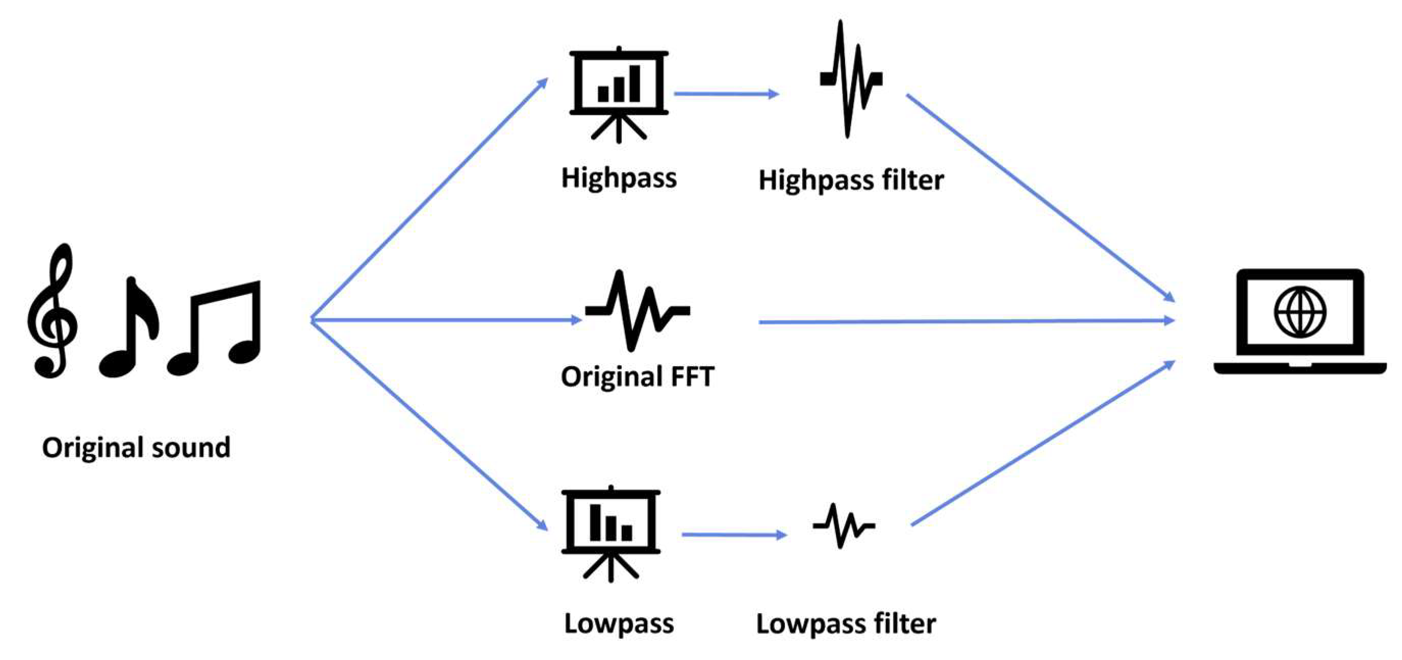
Figure 2.
Python code that calculates the STFT
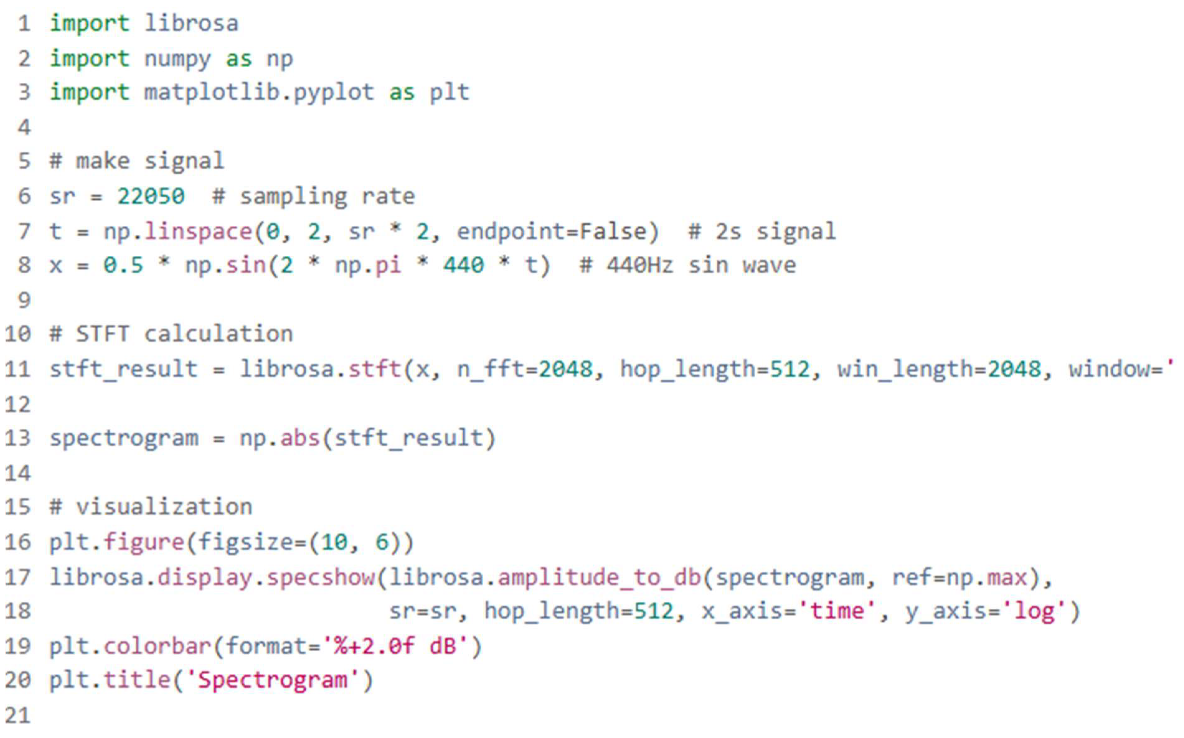
Figure 3.
Python code for calculating the automatic correlation function of the signal
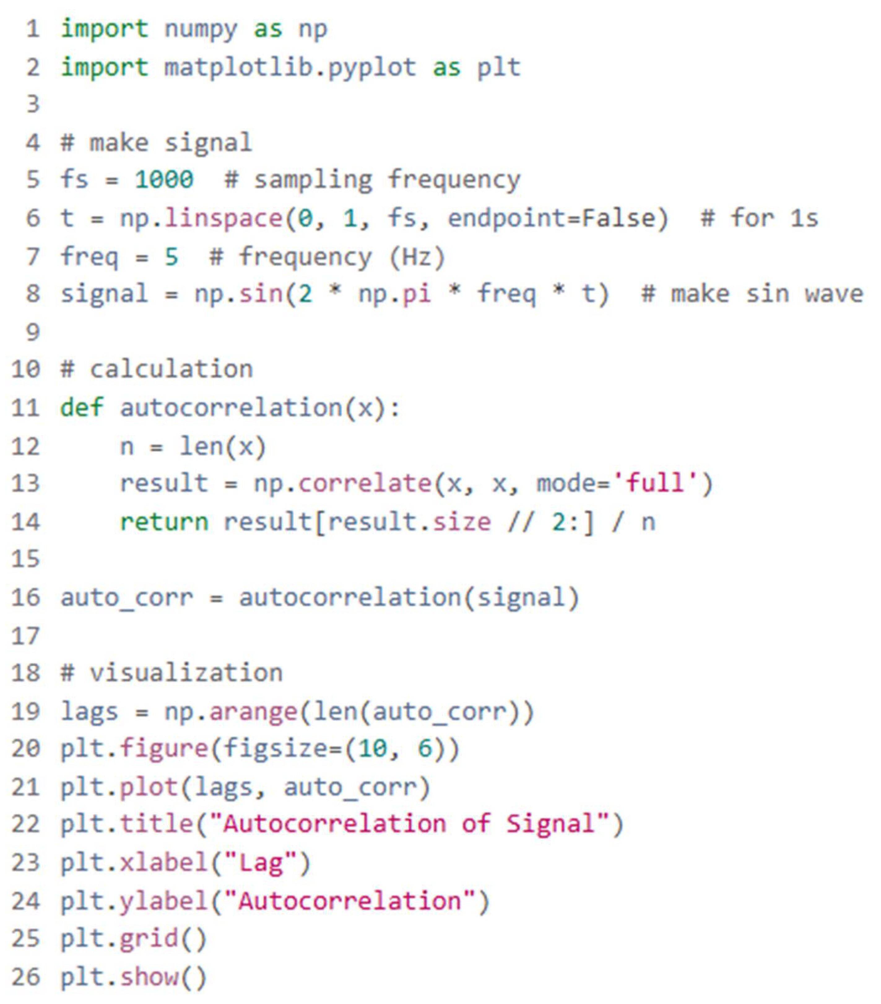
Figure 4.
Implementing NMF using Python code
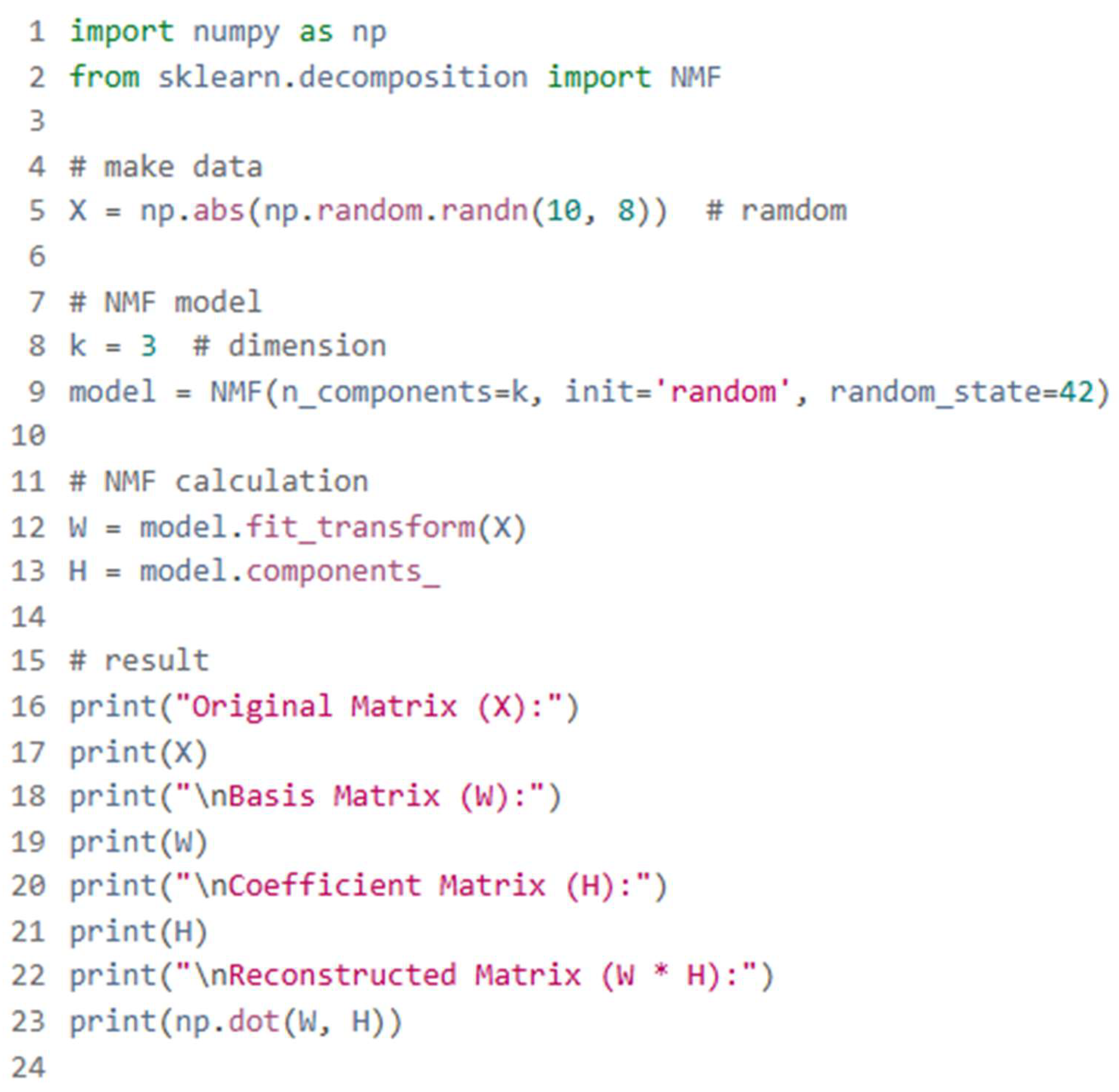
Figure 5.
Sound waves of (a)Jekal and (b)Ku.
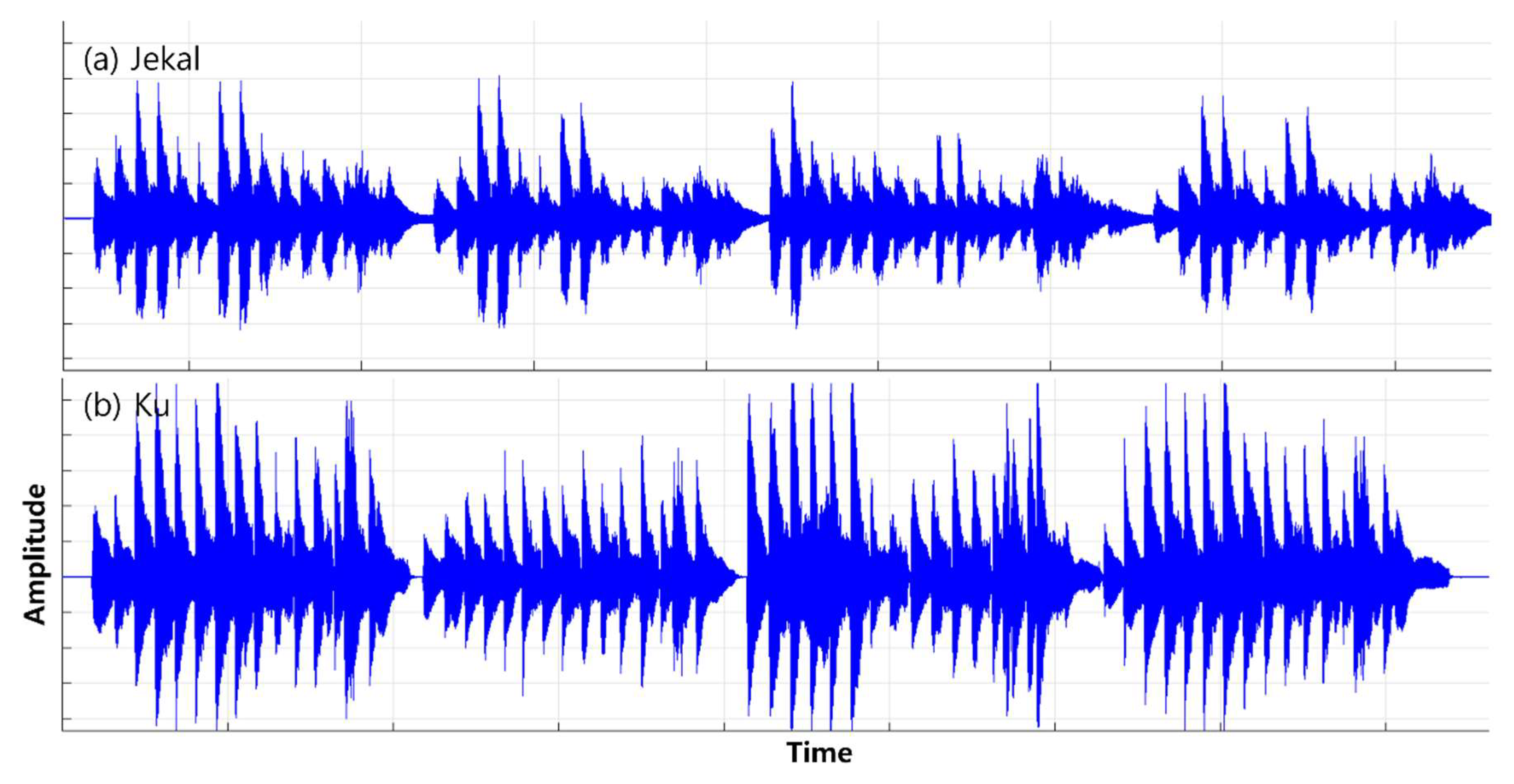
Figure 6.
Sound volume of (a)Jekal and (b)Ku.
Figure 7.
Differential graphs of waveforms for velocity analysis.
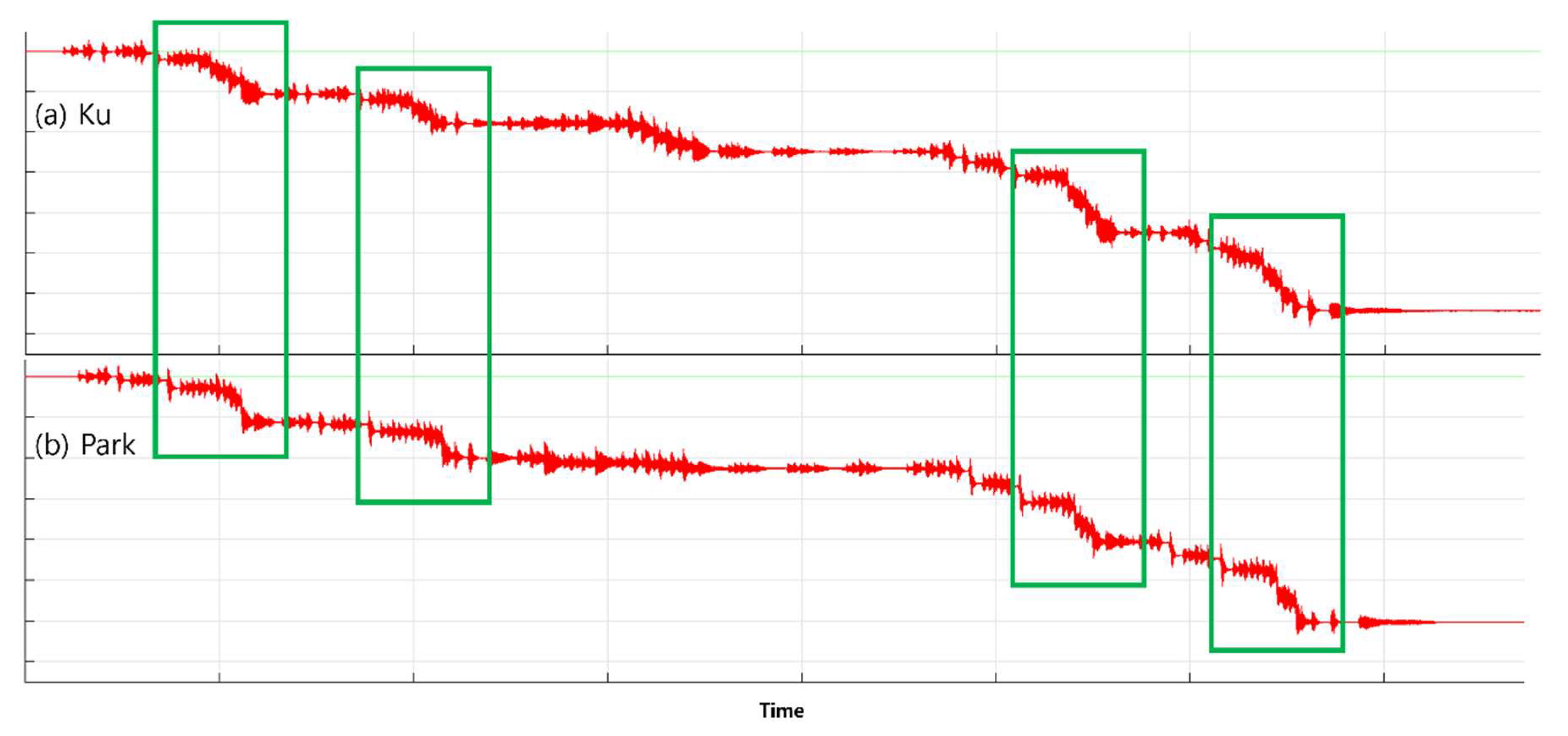
Figure 9.
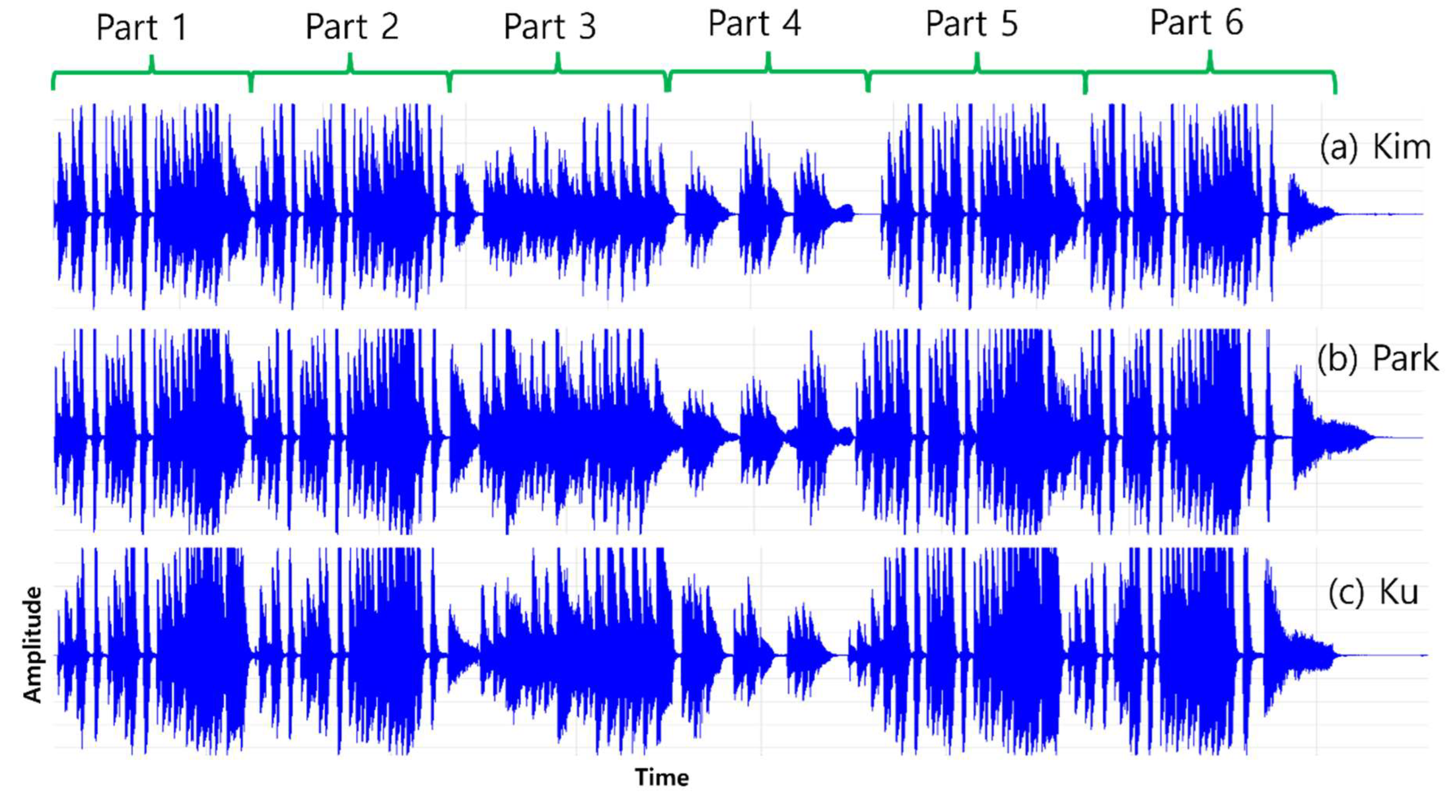
Figure 10.
Disclaimer/Publisher’s Note: The statements, opinions and data contained in all publications are solely those of the individual author(s) and contributor(s) and not of MDPI and/or the editor(s). MDPI and/or the editor(s) disclaim responsibility for any injury to people or property resulting from any ideas, methods, instructions or products referred to in the content. |
© 2025 by the authors. Licensee MDPI, Basel, Switzerland. This article is an open access article distributed under the terms and conditions of the Creative Commons Attribution (CC BY) license (http://creativecommons.org/licenses/by/4.0/).
Copyright: This open access article is published under a Creative Commons CC BY 4.0 license, which permit the free download, distribution, and reuse, provided that the author and preprint are cited in any reuse.


