Neural Networks for Statistical Modeling: Achieving Highly Accurate Chemical Oxygen Demand Prediction in Herbicide-Contaminated Wastewater

1. Introduction

The widespread use of fertilizers and pesticides in agriculture, particularly herbicides, poses a significant threat to water quality. Herbicides are the most extensively employed class of pesticides and are recognized as persistent organic pollutants due to their low biodegradability. During their biotic and abiotic transformations in soil, herbicides form complex metabolites that can infiltrate groundwater at relatively high concentrations, raising concerns about potential human health risks [1,2]. Consequently, the global scientific community has intensified its focus on developing effective treatment methods for herbicide-contaminated wastewater.

Over the past two decades, the worldwide consumption of herbicides has escalated, compounding worries about their environmental fate and slow decomposition rates [3]. Advanced oxidation processes (AOPs) have gained traction as a promising solution for degrading commercial herbicides. For example, the tandem process of sonolysis and photocatalysis (sonophotocatalysis), which employs an ultrasound source of 20 kHz combined with UV light, has shown notable efficacy in degrading herbicides such as alazine and gesaprim [4,5]. These approaches have achieved nearly complete mineralization of active compounds when ultrasound is used alongside a TiO₂ catalyst, highlighting the potential of sonophotocatalysis in mitigating herbicide pollution.

Despite these promising results, the sonophotocatalytic degradation of commercial herbicides remains complex, influenced by factors such as radiant energy balance, spatial distribution of absorbed radiation, and the generation of radical species. Given the nonlinear and multifaceted nature of the degradation process, traditional linear modeling methods often fall short [6,7]. To address this limitation, researchers have turned to more sophisticated computational approaches, particularly artificial intelligence (AI) techniques.

Among AI methods, Artificial Neural Networks (ANNs) are especially suited for predicting water quality and simulating complex treatment processes [8,9]. By capturing both linear and nonlinear relationships without requiring explicit mathematical formulations, ANNs can effectively model intricate photochemical and sonophotocatalytic systems [10,11]. Over the past decade, ANN-based models have seen widespread use in environmental engineering, including photochemical water treatment [12], activated sludge processes [13], real-time control in wastewater treatment plants [14], dye removal via AOPs [15,16], and river pollution monitoring through biochemical oxygen demand analysis [17].

Recent investigations have further demonstrated the utility of ANNs for modeling herbicide degradation in AOPs. Examples include optimizing solar photo-Fenton processes for herbicide mixtures [18] and modeling the TiO₂-mediated photocatalytic degradation of atrazine [19]. However, few studies have thoroughly explored ANN-based approaches for predicting and optimizing sonophotocatalytic processes.

In this context, the present work pursues two main objectives. First, we develop a multilayer feed-forward neural network trained with various backpropagation algorithms to reliably predict Chemical Oxygen Demand (COD) removal during the sonophotocatalytic degradation of alazine and gesaprim herbicides in TiO₂ suspensions under UV irradiation. Second, we perform a sensitivity analysis to identify the most influential parameters governing COD removal efficiency.

Overall, this study contributes to the growing body of literature on AI-driven environmental remediation, emphasizing ANN’s capability for modeling and optimizing AOPs in herbicide-laden wastewater. By harnessing the predictive strength of ANNs and employing systematic sensitivity analyses, we aim to advance the design and operational strategies of wastewater treatment processes, ultimately improving their efficiency and effectiveness for large-scale applications.

2. Related Works

This section reviews significant research on herbicide degradation, wastewater treatment, and the application of Artificial Neural Networks (ANNs) in these fields. Numerous studies have demonstrated the effectiveness of ANNs in modeling complex environmental processes, including water quality monitoring, real-time plant operation, and advanced oxidation processes (AOPs).

2.1. ANN Applications in Wastewater Treatment

Several researchers have explored ANN-based frameworks to enhance wastewater treatment operations. For instance, an ANN-driven intelligent monitoring system was proposed to track key variables in real-time [13], underscoring the role of machine learning in improving both monitoring and control. Similarly, another study utilized a hybrid ANN–genetic algorithm approach to model and optimize activated sludge bulking [14], illustrating how ANNs can be combined with optimization techniques to address operational challenges in wastewater plants.

2.2. ANN Models for Predicting Water Quality Parameters

The predictive capabilities of ANNs have also been widely employed in modeling specific water quality indicators. In one study, ANNs were coupled with response surface methodology to model dye removal by adsorption onto water treatment residuals [15], showcasing the synergy between ANNs and statistical modeling tools. Other work successfully applied ANNs to predict the combined toxicity of phenol and cadmium in wastewater treatment [16], demonstrating their ability to handle multi-component systems. A broader review of machine learning applications in water quality management further highlighted ANNs as a robust tool for both prediction and optimization [17].

2.3. ANNs in Herbicide Degradation and Advanced Oxidation Processes

Moving toward herbicide-specific applications, ANNs have been employed to optimize solar photo-Fenton processes for degrading herbicide mixtures [18]. This research is particularly pertinent to AOPs, revealing how neural network–based models can facilitate more efficient pollutant breakdown. A comprehensive review of AOPs also emphasized the integration of ANNs with two- and multi-way calibration methods, reinforcing the value of neural networks in managing the inherent complexity of oxidation processes [19].

2.4. Environmental Fate of Herbicides

Studies focusing on herbicide persistence underscore the importance of advanced treatment technologies for contaminated waters [1,2]. In addition to environmental impact considerations, food safety concerns drive ongoing efforts to develop more effective and sustainable remediation strategies [3]. These findings further validate the need for targeted research on innovative degradation methods.

2.5. Advanced Oxidation Processes for Herbicide Degradation

Sonophotocatalysis, involving simultaneous ultrasound and photocatalytic treatment, has shown promise for degrading persistent herbicides [4,5]. These processes are inherently complex, involving radical generation, energy transfer, and a multitude of reaction pathways. Consequently, modeling them requires sophisticated data-driven tools such as ANNs to capture nonlinear interactions and optimize operational parameters.

Uniqueness of the Present Work

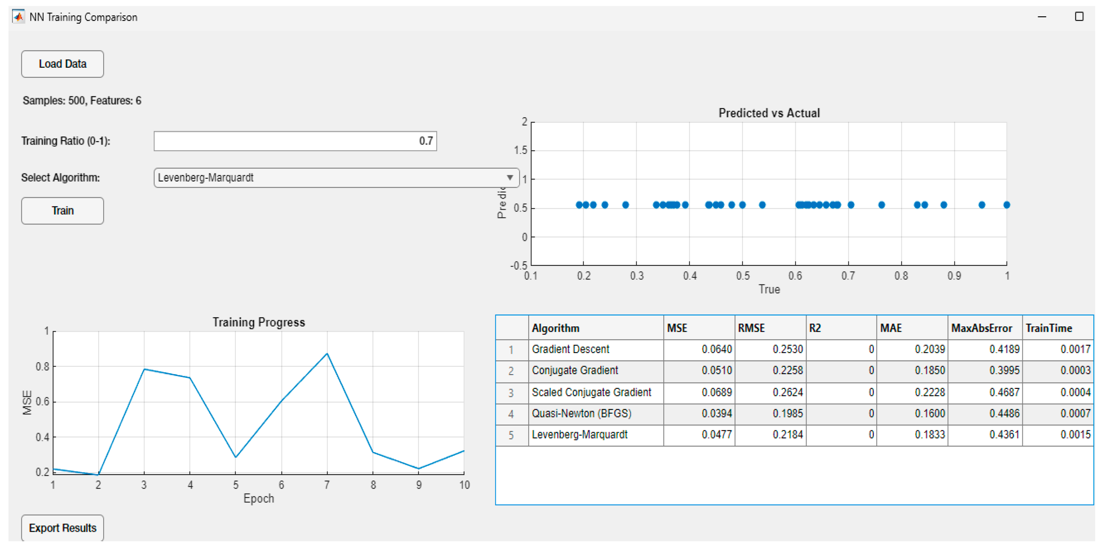
While the aforementioned studies highlight the growing importance of ANNs for wastewater treatment and herbicide degradation, none directly compare to the specific aims of this work. Here, we focus on evaluating multiple backpropagation algorithms within ANN models to predict Chemical Oxygen Demand (COD) removal during the sonophotocatalytic degradation of commercial herbicides. Additionally, we integrate a sensitivity analysis to pinpoint the most influential parameters governing COD removal. Furthermore, unlike previous approaches, we have developed a detailed “Neural Networks for Statistical Modeling” methodology, accompanied by a comprehensive Graphical User Interface (GUI) and advanced statistical tests, specifically tailored to scientifically predict the degradation of commercial herbicides. This distinctive combination of algorithmic comparison, in-depth statistical modeling, parameter sensitivity analysis, and user-friendly tools provides novel insights into optimizing herbicide degradation processes, thereby contributing a fresh perspective to the existing body of research.

3. Materials and Methods

3.1. Chemicals

The commercial herbicides used in this study were Alazine (30/18 LM) and Gesaprim (90 GDA), both obtained directly from Syngenta Crop Protection Inc. (USA). Alazine (30/18 LM) is a complex formulation that contains 30% w/v of alachlor (2-chloro-2’,6’-diethyl-N-methoxymethylacetanilide) and 18% w/v of atrazine (2-chloro-4-ethylamino-6-isopropylamino-1,3,5-triazine) along with various formulating agents. Gesaprim (90 GDA), on the other hand, comprises 90% w/w atrazine and is widely employed for pre- and post-emergence weed control in numerous crop systems.

Titanium dioxide (TiO₂) Degussa P25—sourced from Sigma-Aldrich without further modification—was used as the photocatalyst. P25 is considered a “gold standard” in photocatalytic research due to its well-documented physicochemical properties and consistent performance in degrading organic pollutants. Sulfuric acid (Sigma-Aldrich) was employed for pH adjustments throughout the experiments, ensuring precise control of reaction conditions.

No additional purification or pretreatment was performed on the chemicals to better simulate real-world conditions, where commercial herbicides are often discharged with their full range of formulating agents. Distilled water (Baxter México S.A.) was used for all experiments to minimize interference from background impurities that could affect either the degradation rates or Chemical Oxygen Demand (COD) measurements.

3.2. Herbicide Degradation Experiments

The experimental design was adapted from a Hach Company protocol [20], allowing for methodological consistency and direct comparability with established wastewater treatment practices. The photodegradation experiments were conducted on both Alazine and Gesaprim in a recirculating photochemical reactor:

3.2.1. Reactor Configuration

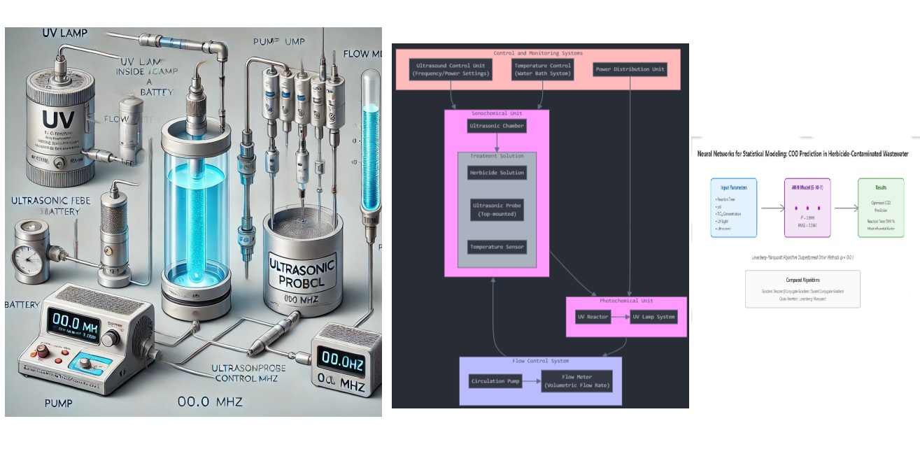
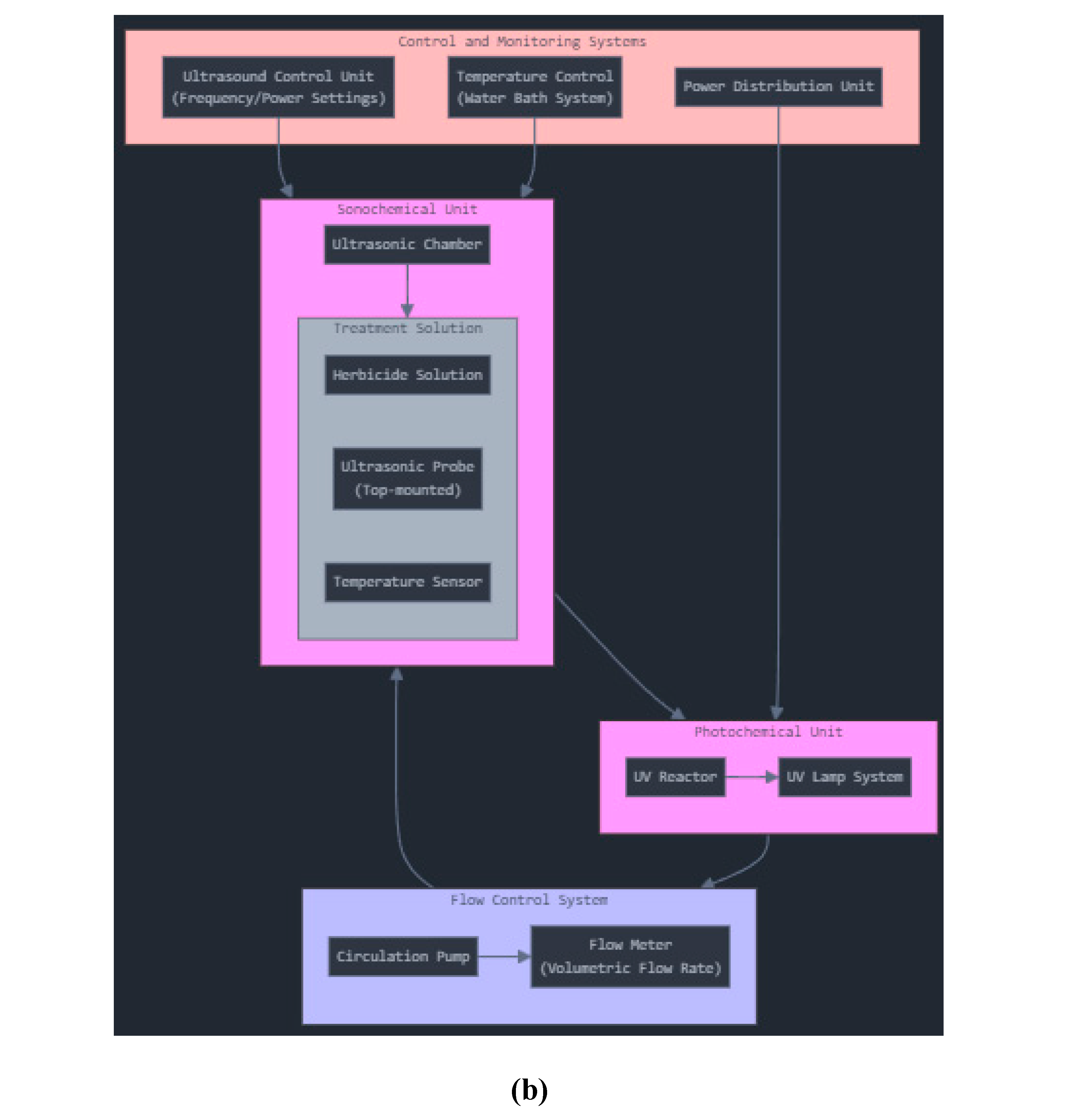
A total volume of 250 mL of herbicide solution was processed at a constant flow rate of 5.63 L·min^-1, ensuring uniform contact of the solution with the photocatalyst and ultrasonic probe. Recirculation-based reactors are widely used benchmarks in photocatalytic research, owing to their reproducible flow patterns and even distribution of reactants.

3.2.2. Ultrasonic Cell Setup

A jacketed ultrasonic cell (150 cm³ capacity) served as the core reaction chamber (Figure 1). Equipped with an ultrasonic probe (500 W, 20 kHz, Cole Parmer), the cell generated high-frequency waves that produced cavitation bubbles. Upon collapse, these bubbles generate localized microenvironments of extreme temperature and pressure, thereby enhancing chemical degradation.

3.2.3. Temperature Control

Water recirculation through the jacketed cell maintained a stable temperature during sonophotocatalysis, isolating the effects of ultrasound and photocatalysis from thermal decomposition. Such temperature regulation is a key step in benchmark experiments, ensuring that observed degradation is attributable to the intended oxidative processes.

3.2.4. UV Irradiation

A 15 W UV lamp (352 nm, Cole Parmer) was positioned to irradiate the reactor contents. The selected wavelength efficiently excites TiO₂, creating electron–hole pairs that drive photodegradation reactions. This approach is a standard method in photocatalytic studies, facilitating direct comparison of results across different laboratories.

3.2.5. Sampling Protocol

Samples were withdrawn at predetermined intervals, ensuring that the total volume removed did not exceed 10% of the initial 250 mL. This minimized disturbances to the reaction kinetics, a practice aligned with established sampling protocols in sonophotocatalytic research.

3.2.6. Sample Filtration and Analysis

➢

Immediately following collection, each sample was filtered to remove suspended TiO₂ particles that might interfere with subsequent analyses. High-Performance Liquid Chromatography (HPLC) was then used to quantify atrazine and alachlor concentrations.

➢

Chemical Oxygen Demand (COD) was measured using standard methods and commercially available Hach COD test tubes, providing a comprehensive overview of the organic load reduction during the degradation process. Adhering to Hach or APHA-based COD protocols ensures that data are consistent with benchmarks in environmental testing.

This integrated approach allowed for a thorough investigation of the sonophotocatalytic degradation of both Alazine and Gesaprim. By leveraging P25 TiO₂, adhering to standardized Hach methodologies, and maintaining precise control over reaction parameters, the study aligns with recognized benchmarks in photocatalytic and environmental engineering research. Consequently, the resulting data on the degradation kinetics of alachlor and atrazine—alongside overall COD reduction—can be reliably compared to similar studies worldwide.

3.3. Sonophotocatalytic Process

Sonophotocatalysis combines sonolysis with TiO₂ photocatalysis under UV irradiation (λ ≤ 400 nm), generating highly reactive oxidant species capable of breaking down toxic, non-biodegradable organic pollutants into relatively harmless end products such as CO₂, H₂O, and mineral acids [18].

In this process, the active herbicide compounds (alachlor and atrazine) adsorbed onto the TiO₂ surface are oxidized by these reactive species. When TiO₂ is illuminated by photons (hν), charge carriers (electron–hole pairs) form, initiating the oxidative reactions that drive pollutant degradation [19]. The simplified mechanism can be represented by Equation (1):

$$Ti{O}_2+h\upsilon \to e_{cb}^{-}+h_{\upsilon b}^{+}$$

(1)

The photogenerated electron–hole pairs (e_cb^-) in the conduction band and (h_vb⁺) in the valence band) migrate to the TiO₂ surface, where they react with species such as H₂O, OH⁻, and O₂ to form highly reactive hydroxyl radicals (·OH), superoxide radicals (O₂·⁻), and hydrogen peroxide (H₂O₂) [20,21]. Simultaneously, ultrasonic irradiation induces cavitation microbubbles, generating localized hot spots with transient high pressures (∼50,000 kPa) and temperatures (∼5,000 K) [22]. The ensuing shock waves enhance mass transfer and further activate the TiO₂ surface, as described in Eq. (2), thereby accelerating the decomposition of the herbicides’ active compounds. Ultimately, these compounds are oxidized by the reactive species formed during sonophotocatalysis, leading to a marked reduction in Chemical Oxygen Demand (COD).

$$\left\{\begin{array}{l}ACTIVE\\ COMPOUNDS\end{array}\right\}+O_2+Ti{O}_2\to C{O}_2+H_{2}O+\left\{\begin{array}{l}MINERAL\\ ACIDS\end{array}\right\}$$

(2)

3.4. Experimental

Alazine contains alachlor, atrazine, and various formulating agents, whereas Gesaprim primarily consists of atrazine and formulating agents. Both herbicide formulations were obtained from Syngenta Crop Protection, Inc. (USA). Titanium dioxide (TiO₂, Degussa P25) and sulfuric acid (H₂SO₄) were of analytical grade (Sigma–Aldrich). Further details on the apparatus, experimental setup, and procedures are provided in [2].

Briefly, a series of photodegradation experiments for each herbicide was carried out in a photochemical reactor operating in recirculating mode, using a total volume of 250 mL at a flow rate of 5.63 L·min⁻¹. The reactor featured a jacketed ultrasonic cell (150 cm³) with an ultrasonic probe (500 W, 20 kHz, Cole Parmer). Temperature control was maintained via water recirculation, and a UV lamp (15 W, 352 nm, Cole Parmer) was used to activate photocatalysis. Samples were withdrawn at predetermined intervals to measure Chemical Oxygen Demand (COD) using standard methods and commercially available test tubes [23].

Table 1 presents the experimental COD values for Alazine and Gesaprim, along with the corresponding reactions for mineralizing the active compounds in each herbicide. The photochemical reactor setup for herbicide removal is illustrated in Figures 1(a) and 1(b).

4. Exploratory Data Analysis

This section presents a comprehensive exploratory data analysis (EDA) of a synthetic herbicide dataset, aiming to uncover distributions, relationships, patterns, and potential data quality issues. The primary goal is to establish a thorough understanding of the dataset, serving as a solid foundation for more advanced modeling. The EDA encompasses eight key tasks:

1.

Data Loading and Inspection

○

The dataset was initially examined by viewing sample rows and assessing structural integrity (e.g., data types, missing values).

○

Summary statistics (mean, median, standard deviation) were computed to provide an initial overview of each variable.

2.

Data Visualization

○

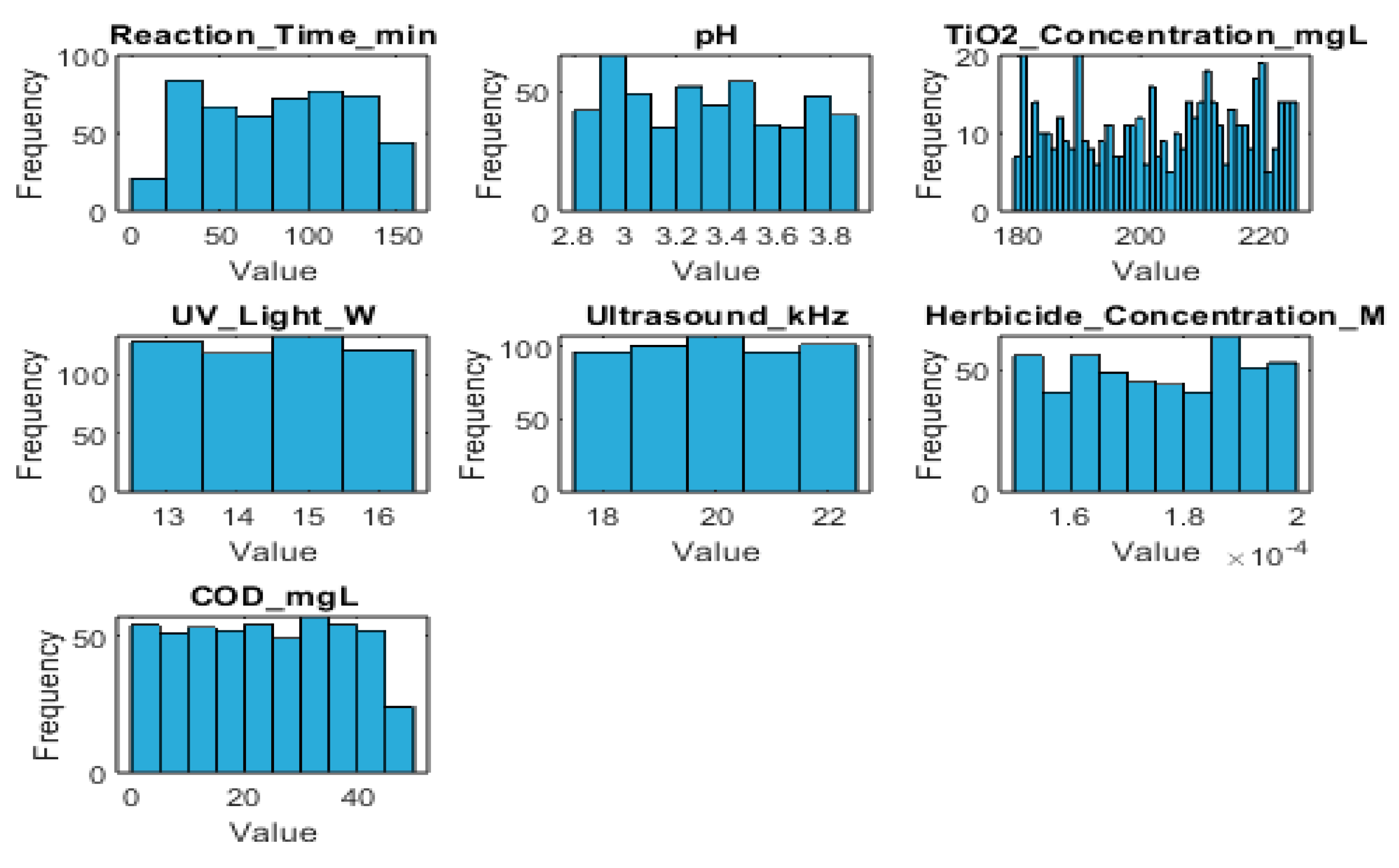
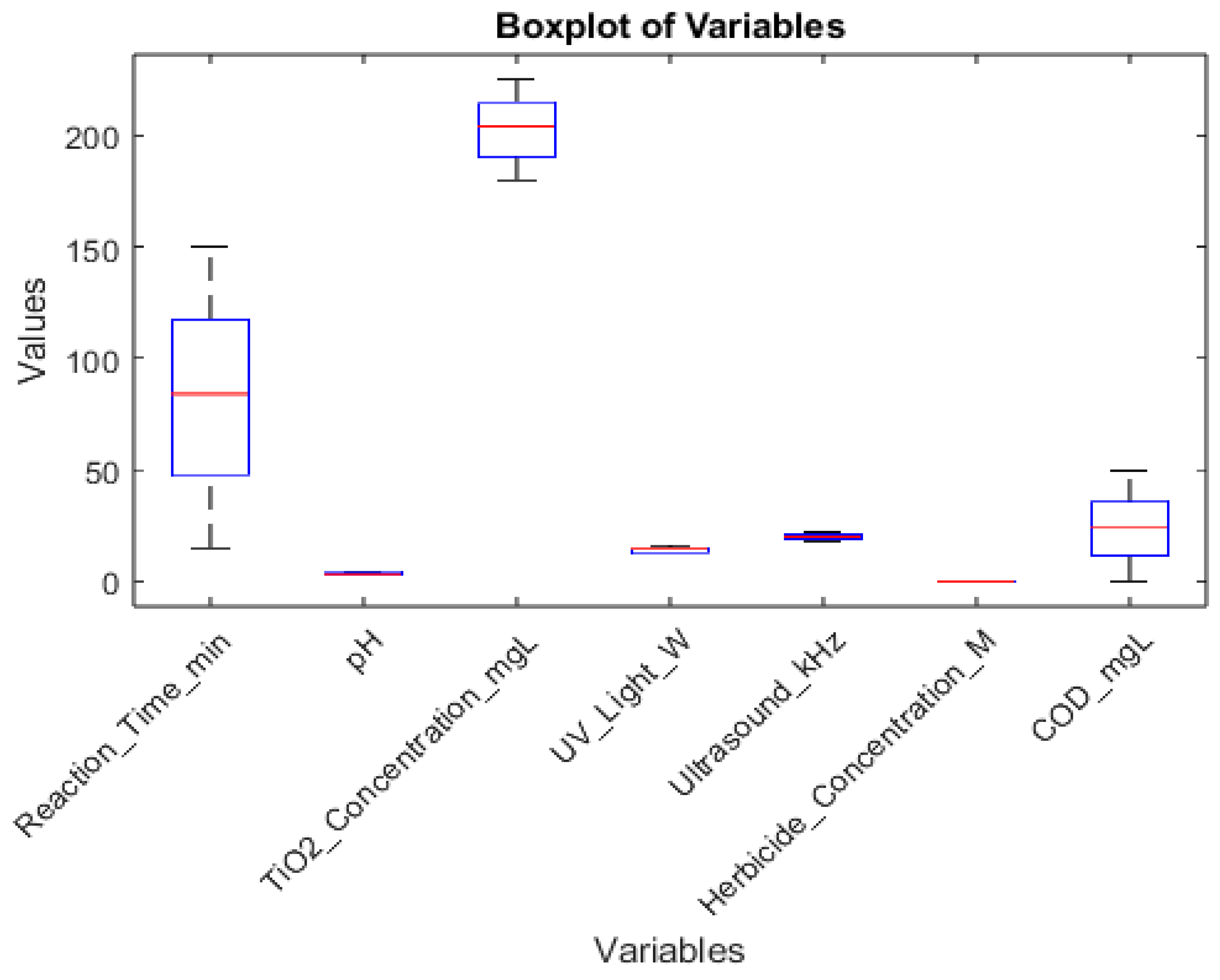
Histograms and box plots were generated for each continuous variable, including Reaction Time (min), pH, TiO₂ Concentration (mg/L), UV Light (W), Ultrasound (kHz), Herbicide Concentration (M), and COD (mg/L).

○

Pair plots and correlation heatmaps were used to illustrate inter-variable relationships.

○

Time series plots captured changes in Herbicide Concentration over Reaction Time, while scatter plots provided insights into pairwise interactions.

3.

Detailed Statistics

○

A correlation matrix offered a visual map of how variables relate to each other.

○

Univariate analysis (density plots, histograms) and bivariate analysis (scatter, box, violin plots) delved deeper into each variable’s distribution and pairwise relationships.

4.

Handling Missing Values

○

Missing data points were identified and visualized.

○

Various imputation strategies (e.g., mean or median imputation) were explored and applied to achieve a complete dataset suitable for analysis.

5.

Outlier Detection

○

Box plots and scatter plots highlighted potential outliers.

○

Identified anomalies were considered for possible exclusion or transformation, depending on their impact on subsequent modeling.

6.

Distribution Analysis

○

Each continuous variable was assessed for normality.

○

Suggested transformations were discussed for variables significantly deviating from normal distributions.

7.

Target Variable Analysis

○

Special attention was paid to the target variable, COD (mg/L).

○

Its distribution and relationships with other variables were thoroughly evaluated and visualized.

8.

Final Summary and Insights

○

The EDA concluded with a synthesis of major findings, highlighting data patterns and quality.

○

These insights set the stage for more informed decision-making in subsequent modeling tasks.

• Dataset Overview

The dataset contains 500 entries and 7 columns, representing the following variables:

• Reaction_Time_min (Integer): Reaction time in minutes.
• pH (Float): pH values.
• TiO2_Concentration_mgL (Integer): Titanium dioxide concentration in mg/L.
• UV_Light_W (Integer): UV light intensity in Watts.
• Ultrasound_kHz (Integer): Ultrasound frequency in kHz.
• Herbicide_Concentration_M (Float): Herbicide concentration in molarity (M).
• COD_mgL (Float): Chemical Oxygen Demand in mg/L.

Next, descriptive statistics—such as mean, median, mode, standard deviation, and range—will be computed for these variables to provide additional insights into the dataset’s structure and variability.

4.1. Descriptive Statistics

A summary of the descriptive statistics for each variable in the dataset is provided below:

1.

Reaction Time (min)

○

Mean: 82.32

○

Median: 84.00

○

Mode: 53.00

○

Standard Deviation: 40.63

○

Range: 15.00 to 150.00 (135.00 total)

2.

pH

○

Mean: 3.33

○

Median: 3.32

○

Mode: 2.95

○

Standard Deviation: 0.31

○

Range: 2.81 to 3.90 (1.09 total)

3.

TiO₂ Concentration (mg/L)

○

Mean: 203.29

○

Median: 204.00

○

Mode: 181.00

○

Standard Deviation: 13.66

○

Range: 180.00 to 225.00 (45.00 total)

4.

UV Light (W)

○

Mean: 14.49

○

Median: 15.00

○

Mode: 15.00

○

Standard Deviation: 1.12

○

Range: 13.00 to 16.00 (3.00 total)

5.

Ultrasound (kHz)

○

Mean: 20.01

○

Median: 20.00

○

Mode: 20.00

○

Standard Deviation: 1.40

○

Range: 18.00 to 22.00 (4.00 total)

6.

Herbicide Concentration (M)

○

Mean: 0.000175

○

Median: 0.000175

○

Mode: 0.000164

○

Standard Deviation: 0.000015

○

Range: 0.000150 to 0.000200 (0.000050 total)

7.

Chemical Oxygen Demand (mg/L)

○

Mean: 23.68

○

Median: 23.77

○

Mode: 0.00

○

Standard Deviation: 13.77

○

Range: 0.00 to 49.53 (49.53 total)

These statistics serve as an essential foundation for comprehending the herbicide degradation process and can guide further experimental design and optimization efforts. Figure 2 presents the histogram frequency distributions for each variable.

Boxplots (Figure 3) are indeed a very effective way to represent the performance of different neural network algorithms, especially when comparing multiple runs. Here's why boxplots are particularly useful in this context:

• Distribution visualization: Boxplots show the entire distribution of results, including the median, quartiles, and potential outliers. This gives a comprehensive view of how each algorithm performs across multiple runs.
• Easy comparison: With boxplots side by side, it's easy to compare the performance of different algorithms at a glance. You can quickly see which algorithms have higher medians, less variability, or more consistent results.
• Variability assessment: The box in a boxplot represents the interquartile range (IQR), which shows the spread of the middle 50% of the data. This helps in understanding how consistent each algorithm is across different runs.
• Outlier detection: Boxplots clearly show outliers as individual points, making it easy to identify runs that performed unusually well or poorly.
• Compact representation: Boxplots can display a lot of information in a compact form, which is especially useful when comparing multiple algorithms or metrics.
• Non-parametric: Boxplots do not assume any underlying distribution of the data, making them suitable for various types of performance metrics.
• Robustness: The median and quartiles used in boxplots are less sensitive to extreme values compared to means, providing a more robust representation of central tendency.

While other representations like bar charts or line plots can be useful for certain aspects, boxplots provide a more comprehensive view of the data distribution, which is crucial when assessing the performance and reliability of different neural network training algorithms across multiple runs.

4.2. Relationships Between Variables

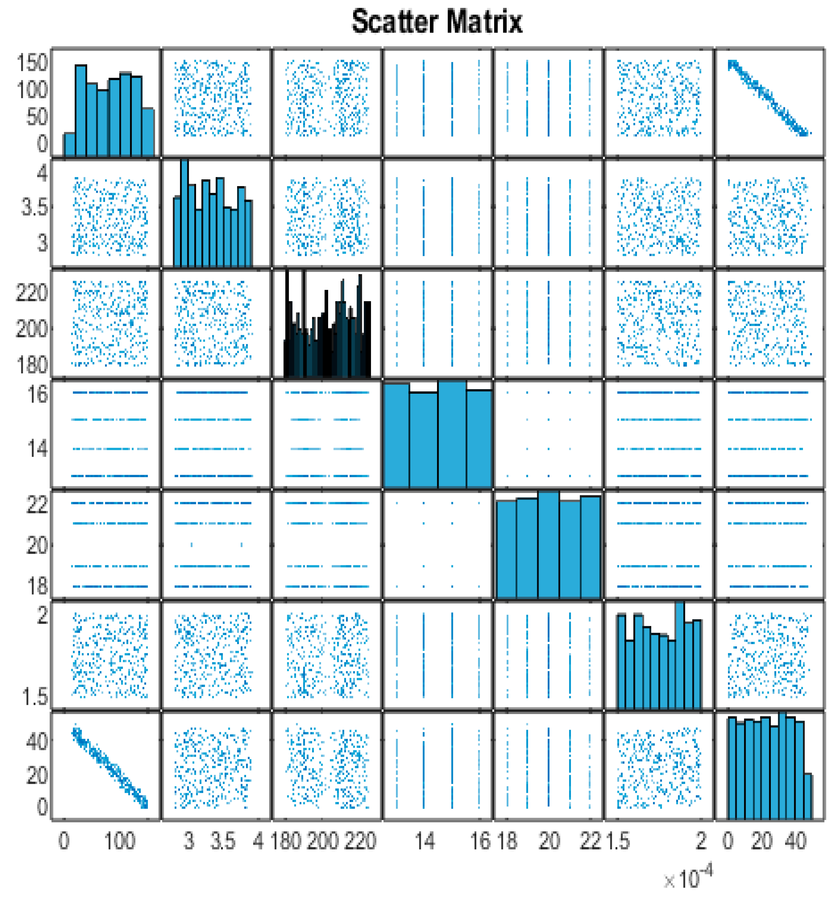
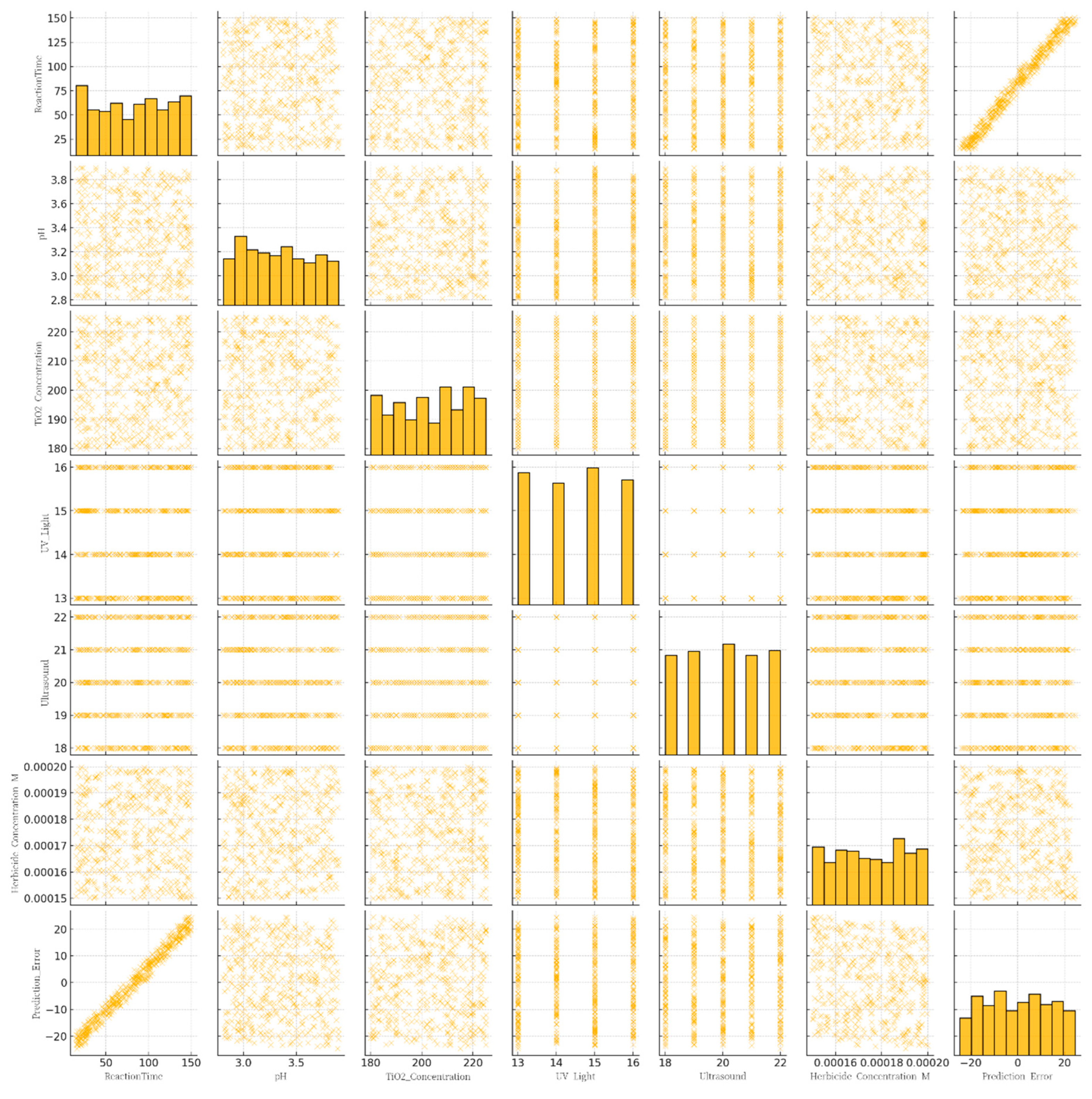
Next, we will create a scatter matrix to visualize the relationships between the variables (Figure 4). The scatter matrix provides a visual representation of the relationships between the variables in the dataset. Each scatter plot shows the relationship between two variables, and the histograms on the diagonal represent the distribution of each variable. However, Figure 5 shows Pair plot of prediction errors across different experimental conditions.

This multi-panel figure displays a pairwise comparison (pair plot) among seven variables: Reaction Time (minutes), pH, TiO₂ Concentration (mg/L), UV Light (Watts), Ultrasound (kHz), Herbicide Concentration (M), and the model’s Prediction Error (COD). Each diagonal cell shows a histogram reflecting the distribution of a single variable, while the off-diagonal cells are scatter plots depicting the relationship between every pair of variables.

• Diagonal Histograms:

  ✓

  Each histogram reveals how frequently particular values occur for the given variable. For example, Reaction Time shows a broad distribution from around 15 to 150 minutes, and TiO₂ Concentration clusters around 180 to 225 mg/L.

• Off-Diagonal Scatter Plots:

  ✓

  The scatter plots allow visual inspection of potential correlations (or lack thereof) between any two variables. For instance, comparing Prediction Error vs. Reaction Time helps reveal if larger errors appear systematically at certain times.

  ✓

  Similarly, you can check pH vs. Prediction Error to see if errors trend higher for more acidic or less acidic conditions.

• Overall Observations:

  ✓

  The plots suggest relatively dispersed (weak) relationships between some variables (e.g., pH vs. TiO₂ Concentration), whereas others might show more discernible patterns.

  ✓

  The inclusion of Prediction Error as one axis in these scatter plots helps identify whether particular operational conditions (e.g., higher TiO₂ concentration, longer reaction time) coincide with larger or smaller model errors.

Together, the pair plot provides a quick, comprehensive overview of variable interactions and highlights where modeling inaccuracies are most pronounced, aiding in refining both data-driven models and experimental setups for COD prediction in herbicide-contaminated wastewater.

Therefore, we will create a parallel coordinate plot to analyze the multivariate data that will discuss in section 8. The parallel coordinate plot allows us to analyze the relationships between multiple variables. Each line represents an observation from the dataset, showing how its values across different variables relate to one another, the lines colored based on the herbicide concentration, indicating how variations in other variables correlate with different levels of herbicide concentration. The plot will help to identify clusters and trends among the observations: as the herbicide concentration increases, there might be distinct patterns in COD_mgL, TiO₂ concentration, and reaction time.

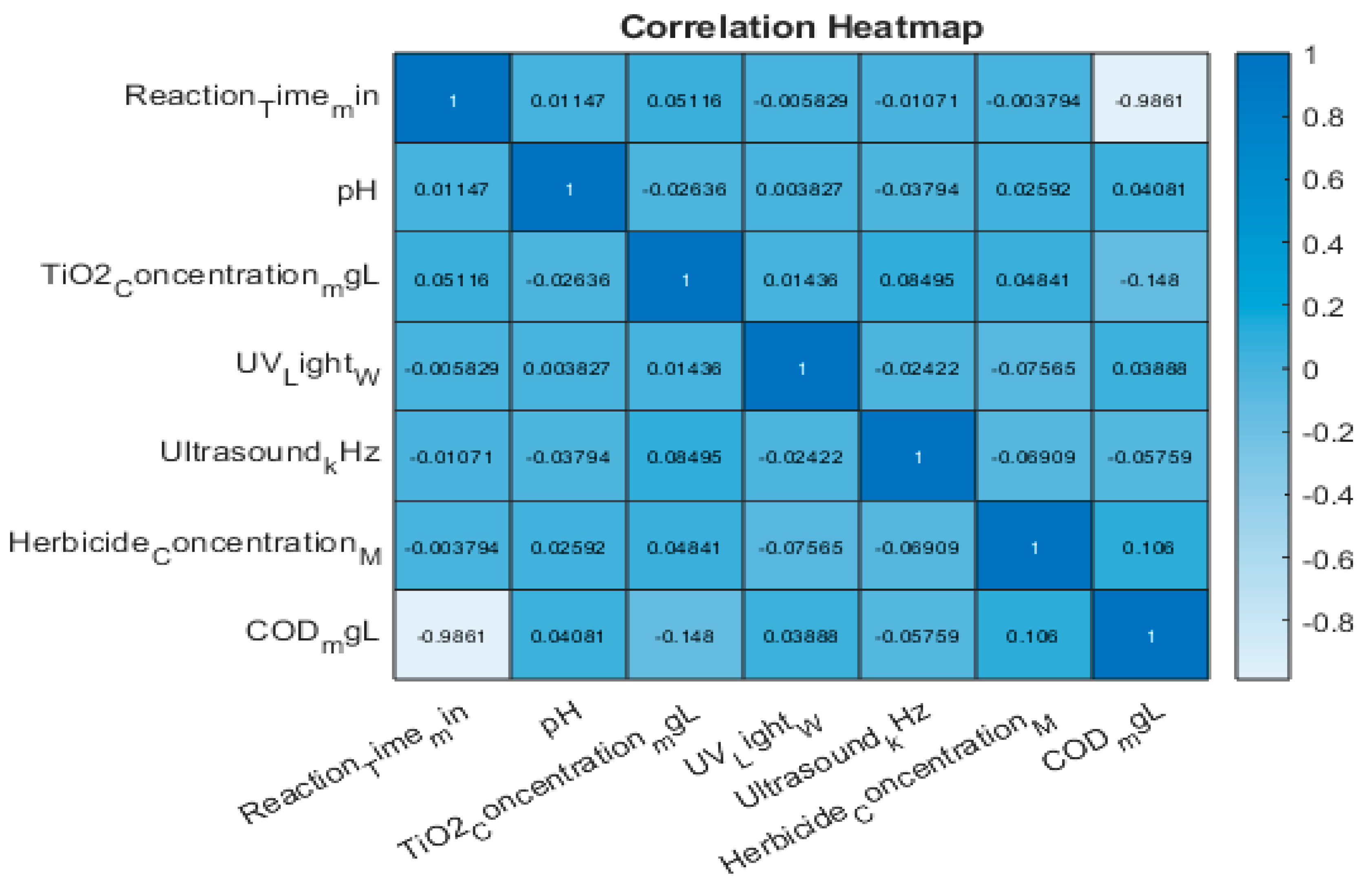
In addition, we will create a heat map based on the Pearson correlation coefficients to identify relationships between the variables that we will discuss extensively in section 7.6.

5. Chemical Oxygen Demand

5.1. The Impact of Reaction Time on Chemical Oxygen Demand Reduction

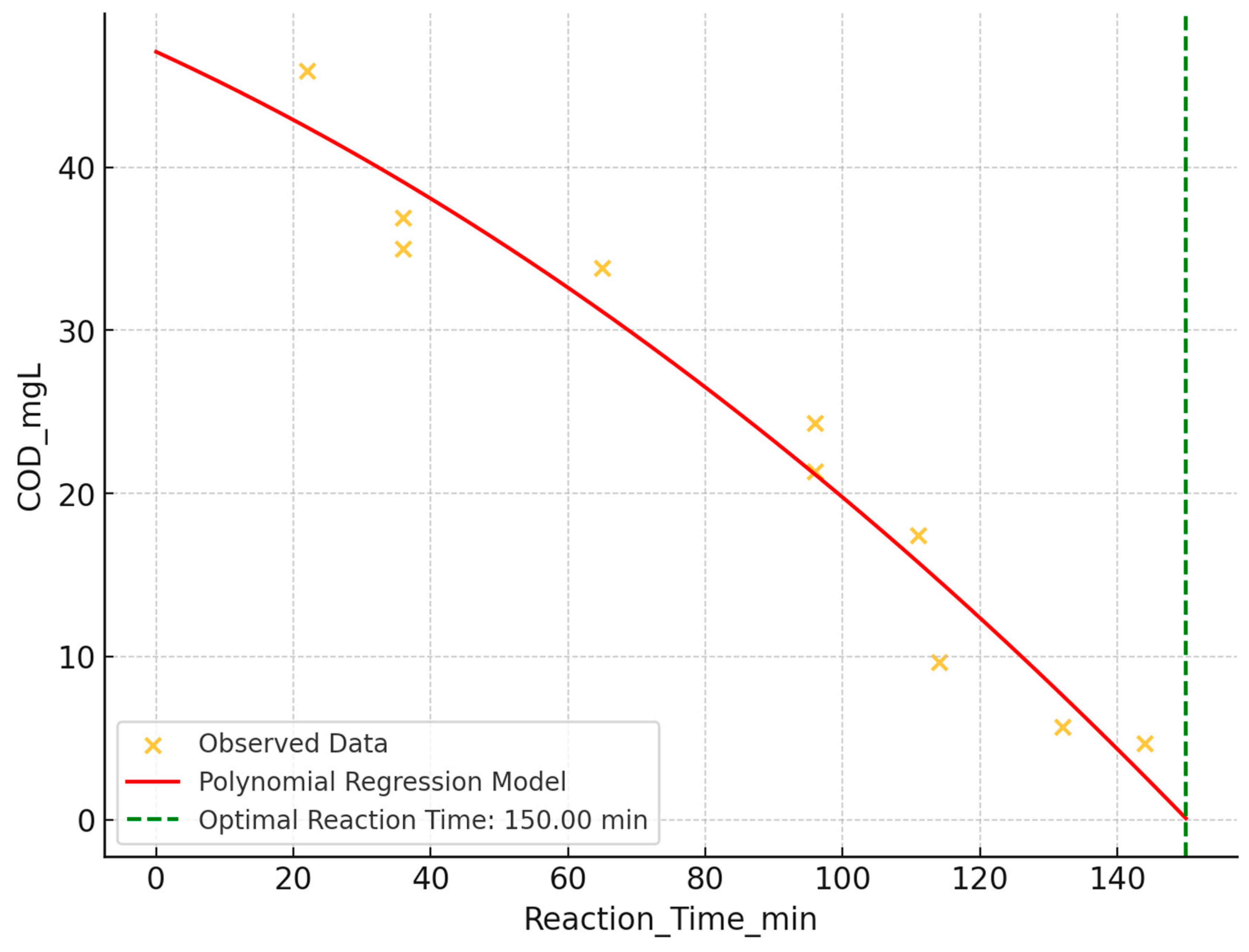
The impact of reaction time on Chemical Oxygen Demand (COD) reduction was analyzed using scatter plot analysis and polynomial regression. A strong negative correlation (r ≈ -0.973) was observed between reaction time and COD levels, indicating significant COD decrease with increased reaction time (Figure 6). The polynomial regression model suggested an optimal reaction time of approximately 150 minutes for minimizing COD levels.

Visual analysis of the scatter plot with polynomial regression overlay revealed a steep reduction in COD at lower reaction times, gradually leveling off at higher reaction times. This supports the finding that longer reaction times correlate with more effective COD reduction, with an optimal point around 150 minutes, after which diminishing returns were observed.

To further refine these results, additional analyses are recommended, including:

• Exploration of higher-degree polynomial or non-linear models for better trend capture.
• Application of piecewise regression to accurately model distinct reaction phases.
• Incorporation of multivariate analysis to account for additional influential variables (e.g., pH, TiO₂ concentration).
• Utilization of model validation techniques and comparison of different models using statistical metrics like Akaike Information Criterion (AIC) or Bayesian Information Criterion (BIC).

These extended analyses could provide deeper insights into the COD reduction process, potentially improving the efficiency and effectiveness of the treatment while considering real-world complexities.

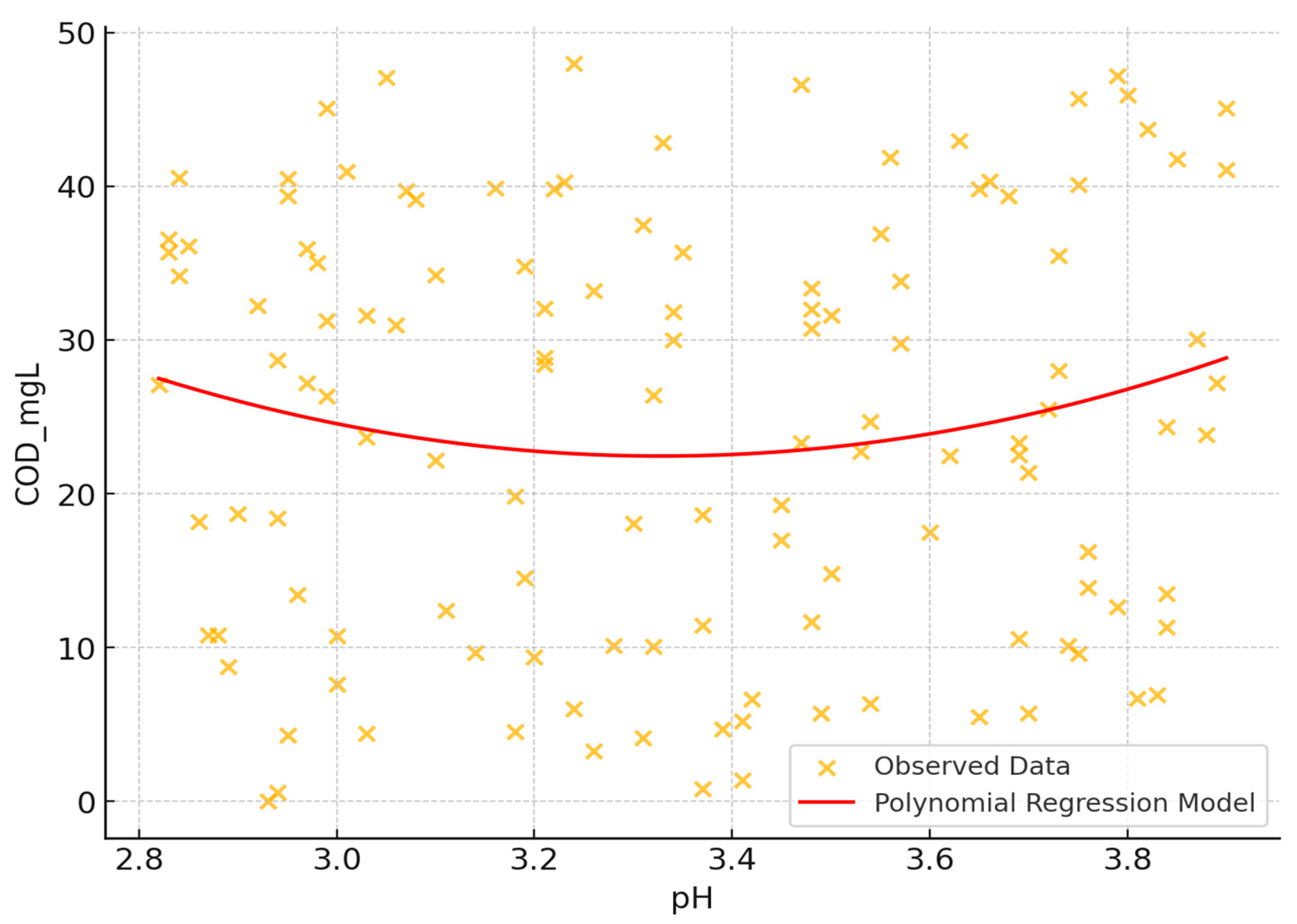
5.2. Investigating the Influence of pH on Chemical Oxygen Demand

The influence of pH on Chemical Oxygen Demand (COD) was investigated using scatter plot analysis and statistical methods. The study examined COD levels ranging from 0 to 50 mg/L across a pH span of 2.8 to 4.0, indicating an acidic environment (Figure 7).

• Key findings:

1.

Correlation analysis: A very weak linear relationship between pH and COD was observed, with a correlation coefficient of approximately 0.026. This suggests that pH alone may not significantly influence COD in a linear manner.

2.

Visual analysis: The scatter plot revealed wide dispersion of data points without a distinct trend, implying that factors other than pH may substantially contribute to COD fluctuations.

3.

Polynomial regression: A second-degree polynomial regression model was fitted to capture potential non-linear relationships. However, given the weak correlation, substantial non-linear effects were not evident.

4.

Optimal pH: No clear optimal pH for minimizing COD was identified, reinforcing that pH might not be the sole factor affecting COD reduction.

5.

Data complexity: Clustered data points and outliers with very low COD values were observed, indicating a complex interaction between pH and COD, possibly involving other variables not depicted in the scatter plot.

These findings highlight the complexity of the pH-COD relationship and suggest that other factors may play significant roles in COD variation.

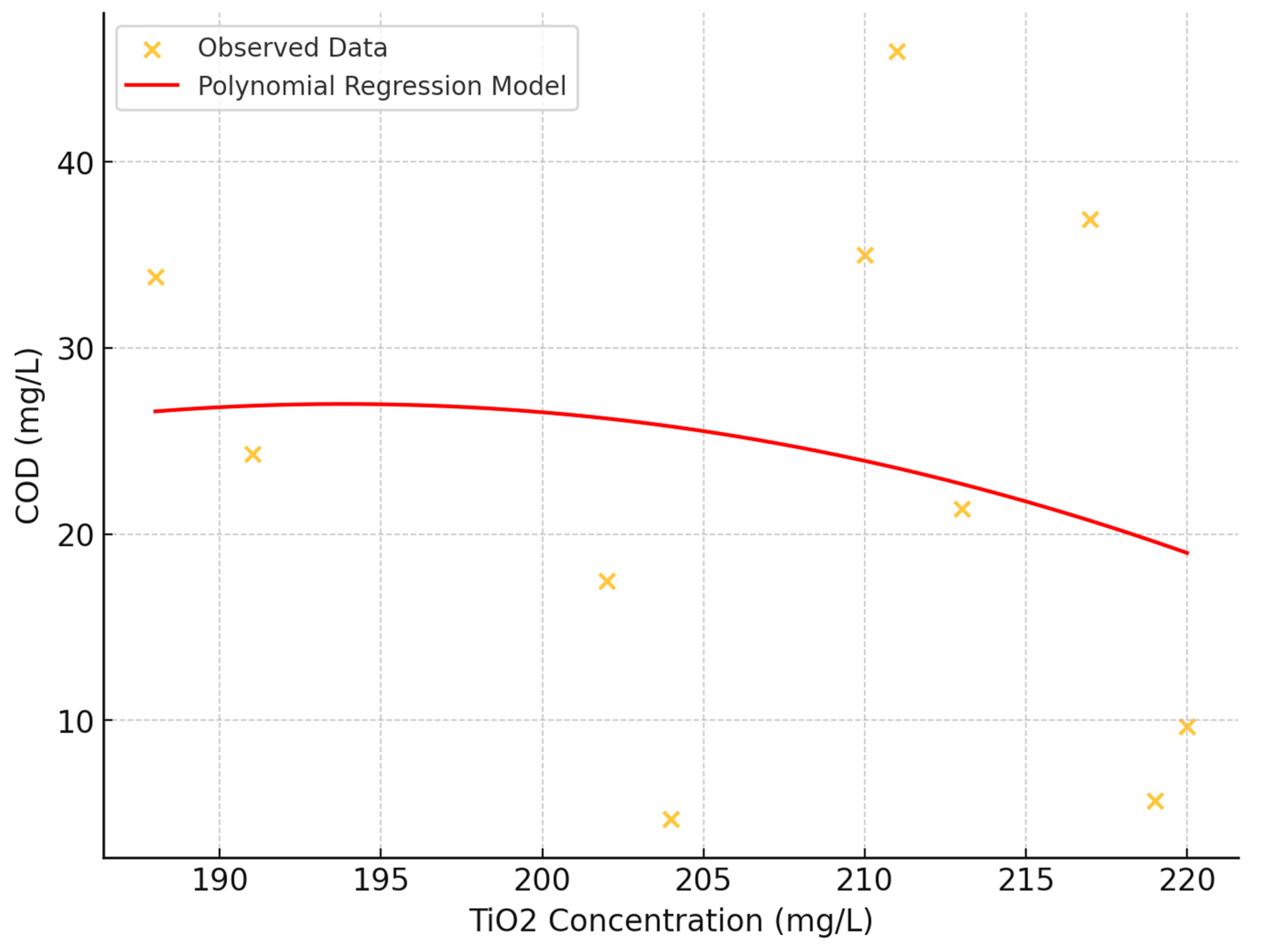
5.3. Evaluating the Impact of TiO₂ Concentration on Chemical Oxygen Demand

The impact of TiO₂ concentration on Chemical Oxygen Demand (COD) was investigated using scatter plot analysis and statistical methods. The study examined TiO₂ concentrations ranging from approximately 180 to 225 mg/L and COD levels from 0 to 50 mg/L (Figure 8).

• Key findings:

1.

Correlation Analysis: A weak negative linear relationship between TiO₂ concentration and COD was observed, with a correlation coefficient of approximately -0.189. This suggests that as TiO₂ concentration increases, there might be a slight tendency for COD values to decrease, though the relationship is not strong.

2.

Visual Assessment: The scatter plot revealed a dispersed arrangement of data points, indicating the absence of a strong linear relationship between TiO₂ concentration and COD. The consistent distribution of COD values across the entire TiO₂ concentration range suggests uniform variability.

3.

Polynomial regression: A second-degree polynomial regression model was fitted to capture potential non-linear relationships. However, no strong, straightforward trend was evident.

4.

Data Complexity: Vertical clustering of data points, particularly at lower COD levels, was observed, potentially indicating underlying experimental or treatment conditions that warrant further exploration.

5.

Absence of Threshold Effect: No distinct outlier pattern or threshold effect was observed where a specific TiO₂ concentration drastically altered COD values.

These findings suggest that while TiO₂ concentration may have a limited direct effect on COD, the relationship is complex and likely influenced by additional factors not captured in this analysis.

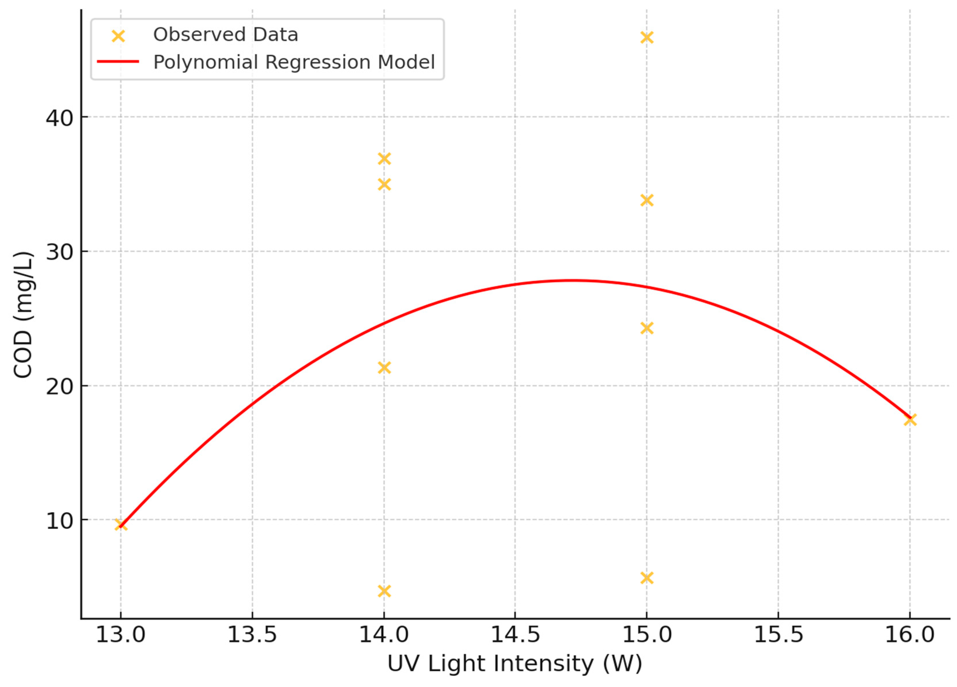
5.4. The Influence of Ultraviolet (UV) Light Intensity on Chemical Oxygen Demand

The impact of Ultraviolet (UV) light intensity on Chemical Oxygen Demand (COD) was investigated using scatter plot analysis and statistical methods (Figure 9). The study examined UV light intensities ranging from 13 to 16 Watts and COD values from 0 to 50 mg/L.

• Key findings:

1.

Correlation analysis: A weak positive linear relationship between UV light intensity and COD was observed, with a correlation coefficient of approximately 0.162. This suggests a slight tendency for COD values to increase with increasing UV light intensity, though the relationship is not strong.

2.

Visual assessment: The scatter plot revealed a consistent spread and pattern of COD values across all levels of UV exposure, indicating that UV light intensity alone may not exert a strong direct influence on COD within the experimental setup.

3.

Polynomial regression: A second-degree polynomial regression model was fitted to capture potential non-linear relationships. However, no clear trend, either linear or non-linear, correlating UV light intensity to COD reduction was observed.

4.

Data distribution: High variability in COD values was observed at each UV intensity level, suggesting that other factors may play a significant role in determining COD beyond the influence of UV light alone.

5.

Absence of threshold effect: No clear threshold effect was observed where variations in UV light intensity significantly altered COD levels.

These findings indicate that while UV light intensity may have a weak positive correlation with COD, the relationship is complex and likely influenced by additional factors not captured in this analysis. The consistent variability across UV intensities suggests that other variables may be more influential in determining COD levels.

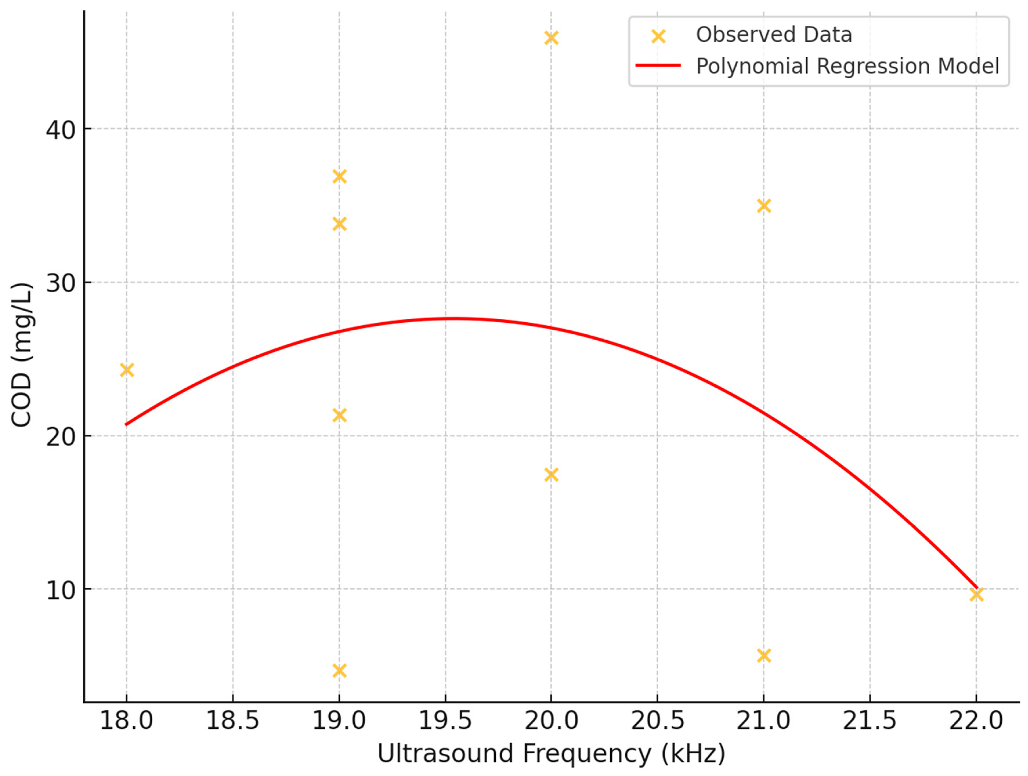
5.5. The Effect of Ultrasound Frequency on Chemical Oxygen Demand (COD)

The impact of ultrasound frequency on Chemical Oxygen Demand (COD) was investigated using scatter plot analysis and statistical methods (Figure 10). The study examined ultrasound frequencies ranging from 18 to 22 Hz and COD values from 0 to 50 mg/L.

• Key findings:

1.

Correlation Analysis: A weak negative linear relationship between ultrasound frequency and COD was observed, with a correlation coefficient of approximately -0.244. This suggests a slight tendency for COD values to decrease as ultrasound frequency increases, though the relationship is not strong.

2.

Visual Assessment: The scatter plot revealed a consistent and wide variance of COD values across all tested frequencies, indicating that variations in ultrasound frequency within the tested range may not exert a significant direct effect on COD.

3.

Polynomial regression: A second-degree polynomial regression model was fitted to capture potential non-linear relationships. However, no discernible trend, either linear or non-linear, emerged between ultrasound frequency and COD levels.

4.

Data Distribution: Data density skewed towards lower COD values at all frequency levels, with fewer instances at higher COD values, suggesting the influence of other factors not captured in this analysis.

5.

Absence of Threshold Effect: No evident threshold effects were observed where specific ultrasound frequencies dramatically altered COD levels.

These findings suggest that while ultrasound frequency may have a weak negative correlation with COD, the relationship is complex and likely influenced by additional factors not captured in this analysis. The consistent variability across frequencies indicates that other variables may play a more significant role in determining COD levels.

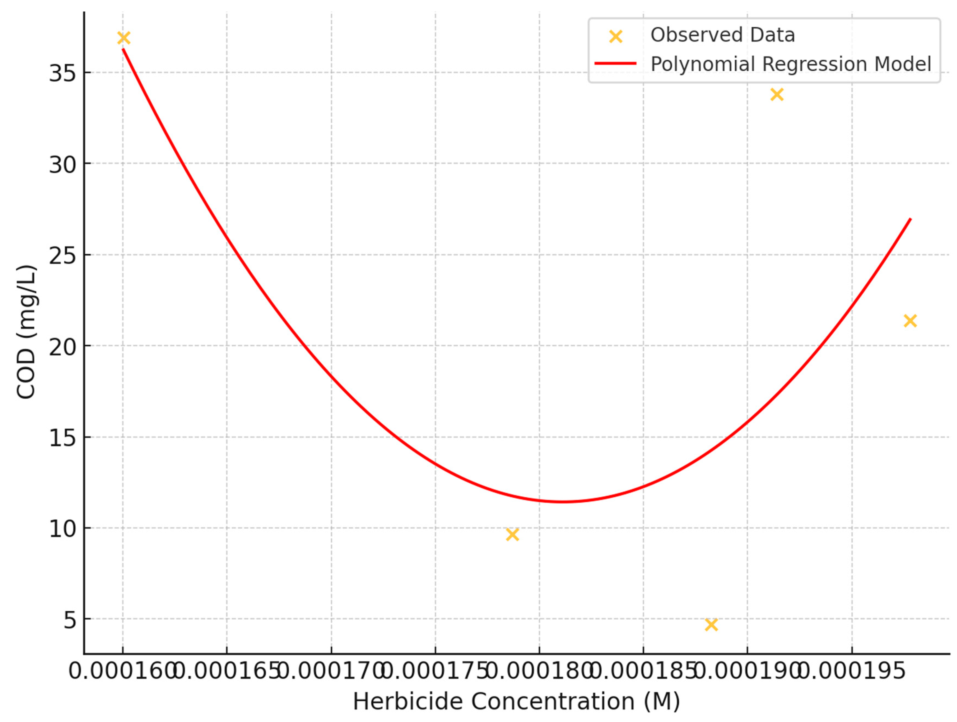
5.6. The Effect of Herbicide Concentration on Chemical Oxygen Demand (COD)

The influence of herbicide concentration on Chemical Oxygen Demand (COD) was investigated using scatter plot analysis and statistical methods (Figure 11). The study examined herbicide concentrations ranging from approximately: $1.5*{10}^{-4}M$ to $2.0*{10}^{-4}M$ and COD values from 0 to 50 mg/L.

• Key findings:

• Correlation Analysis: A moderate negative linear relationship between herbicide concentration and COD was observed, with a correlation coefficient of approximately -0.346. This suggests a tendency for COD values to decrease as herbicide concentration increases, though the relationship is not overly strong.
• Visual Assessment: The scatter plot revealed a dispersed pattern of data points across the plot, indicating no evident strong linear or non-linear relationship between herbicide concentration and COD.
• Polynomial regression: A second-degree polynomial regression model was fitted to capture potential non-linear relationships, helping to visualize nuanced trends beyond simple linear relationships.
• Data Distribution: A slightly higher density of data points was noted in the lower to mid-range of COD values (10-30 mg/L) across all herbicide concentrations, suggesting potential complex interactions or influences from variables not captured in this analysis.
• Absence of Threshold Effect: No distinct threshold effect was observed where dramatic changes in COD occurred at specific herbicide concentrations.

These findings suggest that while herbicide concentration may have a moderate negative correlation with COD, the relationship is complex and likely influenced by additional factors not captured in this analysis. The consistent variability across concentrations indicates that other variables may play significant roles in determining COD levels.

6. Artificial Neural Network

Inspired by the intricate architecture of the human brain, artificial neural networks consist of neurons organized into distinct layers, with each connection between neurons carrying a unique weight that influences the network's function. Much like in nature, the strength and pattern of these connections are vital in shaping the network's behavior. A commonly used structure for function approximation is the multi-layer perceptron, often referred to as a feed-forward network. This type of network typically features one or more hidden layers composed of sigmoid neurons, followed by an output layer of linear neurons. The hidden layers enable the network to capture both nonlinear and linear relationships between inputs and outputs, while the linear output layer allows the network to generate values beyond the constrained range of –1 to +1. In the realm of neural networks, a two-layer notation is often employed for such configurations, reflecting the layered complexity and potential for learning inherent in these systems. Table 2 shows Neural Networks Model Development Workflow.

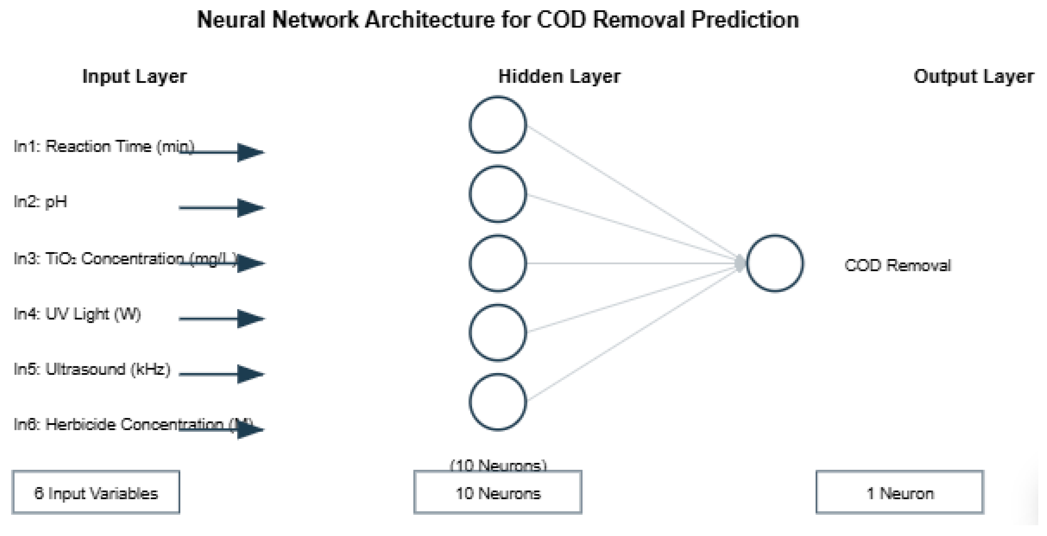
The number of neurons in the input and output layers is given respectively by the number of input and output variables in the process under investigation. In this work, a feed-forward is proposed, the input layer consists of nine variables (reaction time, pH (potential of hydrogen), TiO₂ , UV light intensity, Ultrasound frecuency (fUS) and herbicide concentration (HC). However, the output layer contains one variable (COD). The optimal number of neurons in the hidden layer(s) n_s is difficult to specify, and depends on the type and complexity of the task. This number is usually determined iteratively. Each neuron in the hidden layer has a bias b (threshold), which was added to the weighted inputs to form the neuron n (Eq. 3). This sum, n, is the argument of the transfer function f.

The number of neurons in the input and output layers was intrinsically tied to the variables we seek to understand within a given process. In this study, we propose a feed-forward network where the input layer encompasses nine key variables: reaction time, pH (potential of hydrogen), TiO₂ concentration, UV light intensity, ultrasound frequency (fUS), and herbicide concentration (HC). These inputs collectively guide the network towards a single output variable—COD. Determining the optimal number of neurons within the hidden layers is a nuanced challenge, influenced by the complexity and nature of the task at hand. This optimal number is typically found through iterative refinement. Each hidden neuron carries a bias (threshold) that, when combined with the weighted inputs, forms the neuron's output (n), which is then passed through the transfer function (f). This process, though technical, echoes the underlying elegance of neural networks in their ability to model and understand complex relationships within data.

A structure capable of being trained with data will be able to follow the model over time. So, a single-layer ANN with inputs $\left(s\right)$ and a single output $COD\left(s\right)$, is proposed. The proposed ANN model with $N$ hidden neurons takes the form:

$$COD\left(s\right)=W_o^T\mathrm{*}\sigma \left(\left(W_i\right)\mathrm{*}s+b_i\right)+b_o$$

(3)

where the column vectors $W_i$ and $W_o$ of size $N$ contain the inputs and output weights, respectively. The same size vector $b_i$ contains the input biases while the scalar $b_o$ contains the output bias. However, the function $\sigma \left(\right)$ stands for the activation function, which, in this case, after some exploration, the hyperbolic tangent sigmoid transfer function was selected, which takes the form as Eq. 4.

$$\sigma \left(x\right)={\displaystyle \frac{e^x-e^{-x}}{e^x+e^{-x}}}={\displaystyle \frac{2}{1+e^{-2x}}}-1$$

(4)

It is applied to all the elements of its input vector $W_{i}s+b_i$, with $N$ which for a network with 10 hidden nodes. While a linear transfer function (PURELIN) was selected for the output layer. Indeed, the activations functions play an essential role in achieving good performance.

If considering the transfer functions, in the account that, the Eq. 5 may be expressed as follows:

$$COD=PURELIN\left\{W_o\times \left[TANSIG\left(W_i\times I{n}_k+b{1}_s\right)\right]+b2\right\}$$

(5)

In this study, a multilayer feed-forward artificial neural network (ANN) with a single hidden layer was employed across all data sets, trained by different kinds of backpropagation algorithms as Gradient Descent Algorithm, Conjugate Gradient Algorithm, Scaled Conjugate Gradient Algorithm, Quasi-Newton Algorithm, Levenberg-Marquardt Algorithm. In the final stage of the design a predictive modeling system, which serves to predict various sets of input data into their respective classes, as showed in Figure 12 and Figure 13, respectively.

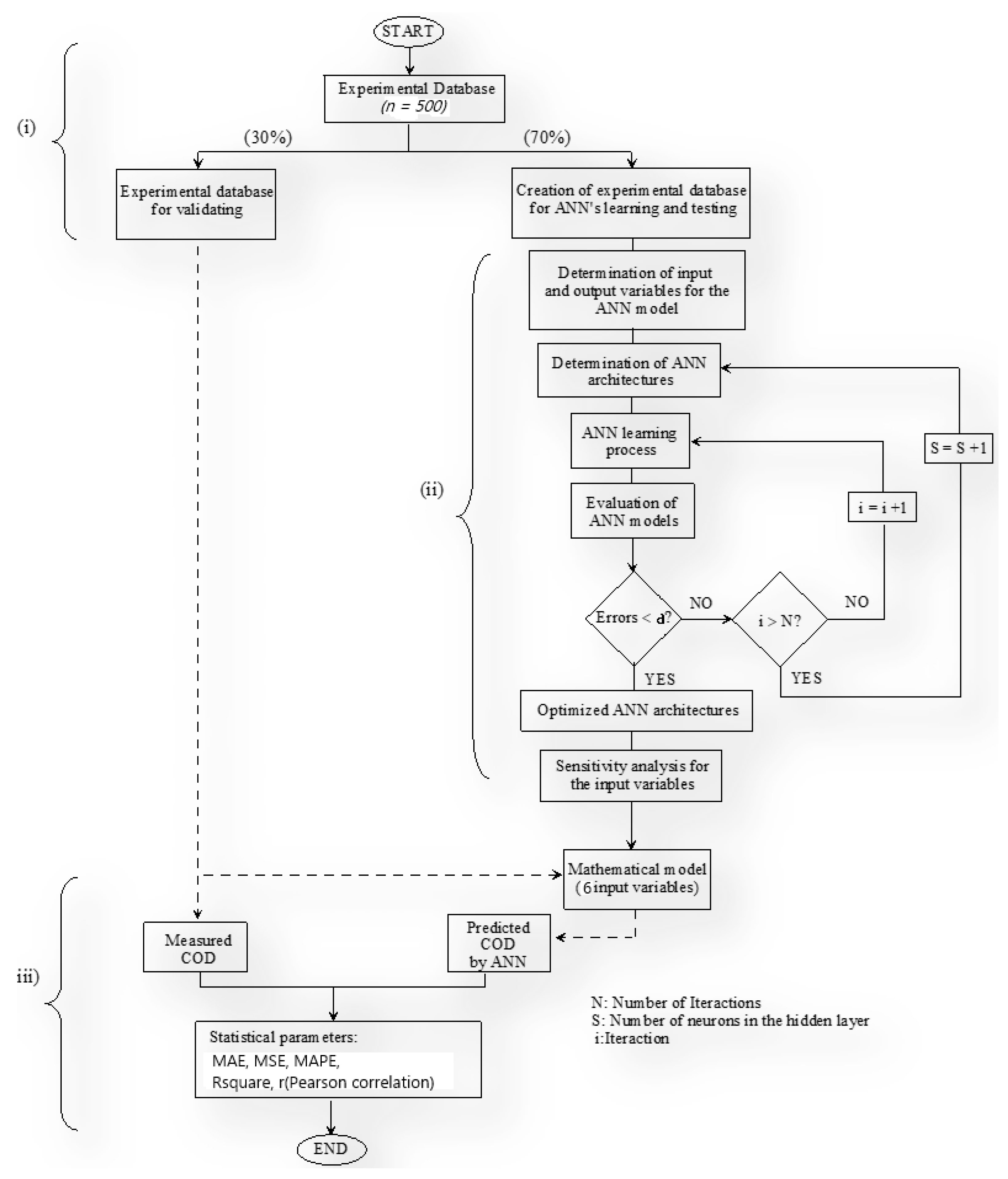
The systematic analysis and reproduction of our methodological flowchart using appropriate formatting and technical specifications.

• Implementation Specifications:
• 1. Initial Data Management Protocol
• %%%
• Data = ExperimentalDB(n=500)
• TrainingSet = Data [0:350] # 70%
• ValidationSet = Data[350:500] # 30%
• %%%
• 2. Architectural Definition Parameters
• %%%
• S: Network architecture parameter
• N: Maximum iteration limit
• i: Current iteration index
• α: Error threshold criterion
• %%%
• 3. Iterative Learning Algorithm
• %%%
• while True:
• error = train_network(S, i)
• if error <α:
• break
• if i > N:
• S = S + 1
• i = 1
• else:
• i = i + 1
• %%%
• 4. Statistical Validation Metrics
• %%%
• MAE = mean(|predicted - measured|)
• MSE = mean((predicted - measured)²)
• MAPE = mean(|predicted - measured|/measured × 100)
• R² = 1 - SSres/SStot
• %%%

This methodological framework ensures systematic optimization of the ANN architecture while maintaining rigorous validation protocols through statistical assessment metrics. The iterative process continues until either convergence criteria are met (error < α) or maximum architectural complexity is reached.

7. Backpropagation Algorithms and Experimental Setup

Backpropagation was developed as a sophisticated enhancement of the Widrow-Hoff learning rule, specifically designed for multi-layer networks and nonlinear differentiable transfer functions. This method has become a cornerstone in training neural networks, allowing them to learn complex patterns and relationships within data. By repeatedly presenting the network with input vectors alongside their corresponding target outputs, backpropagation adjusts the network’s internal weights, guiding it to approximate intricate functions with increasing accuracy. This iterative process not only helps the network to associate specific input vectors with their correct outputs but also enables it to classify and generalize new inputs in ways that are meaningful and precise, as defined by the parameters you set.

The beauty of backpropagation lies in its ability to refine the network's understanding layer by layer, gradually reducing the error between the predicted and actual outputs. Through this method, the network learns to navigate the complexities of nonlinear relationships, adapting its internal structure to reflect the underlying patterns of the data. This powerful technique has proven indispensable in a wide range of applications, from function approximation to classification tasks, making it a fundamental tool in the advancement of neural network research [22].

• In summary, we use five training algorithms to solve the modeling problem:

Gradient Descent Algorithm, Conjugate Gradient Algorithm, Scaled Conjugate Gradient Algorithm, Quasi-Newton Algorithms and Levenbergo-Marquardt Algorithm [23,24,25,26,27,28]. For each algorithm, we performed 30 independent runs. The choice of 30 runs in the neural network training process is based on statistical principles and practical considerations in machine learning. Here's why 30 runs are often used:

✓

Statistical significance: In statistics, 30 often considered the minimum sample size for the Central Limit Theorem to apply. This theorem states that the distribution of sample means approximates a normal distribution as the sample size becomes large, regardless of the population's distribution.

✓

Reducing randomness: Neural network training involves random initialization of weights and often random sampling of data. Multiple runs help to average out the effects of this randomness, providing a more reliable estimate of the model's performance.

✓

Assessing variability: With 30 runs, you can get a good sense of the variability in model performance. This helps in understanding how stable the results are across different initializations and data splits.

✓

Balancing computation time and reliability: While more runs (e.g., 100 or 1000) would provide even more reliable results, 30 runs strike a balance between computational efficiency and statistical robustness.

✓

Common practice: In machine learning and neural network research, 30 runs have become a common practice, making results more comparable across different studies.

However, the number of runs can be adjusted based on specific needs, computational resources, or the complexity of the problem. In some cases, fewer runs might be sufficient, while in others, more runs might be necessary for higher confidence in the results. In each run, the problem data was split into a training and testing set, where the former contains 70% of the data samples and the latter 30%. The datasets were randomly partitioned before each run, and while training performance will be reported the critical result will be the prediction accuracy of the evolved models over the test data. In particular, the algorithms were compared using the Mean Squared Error (MSE) and the coefficient of determination (R²), computed over the ground truth output and the estimated output of each algorithm, for the training and testing data. Table 3 summarizes all parameters for five backpropagation algorithms. We will also report an analysis of the size of the solutions generated by the algorithms that achieved the best performance, as an approximation of model complexity.

Table 3, Table 4, Table 5 and Table 6, highlighted parameters for Gradient Desent Algorithm, Conjugate Gradient Algorithm, Scaled Conjugate Gradient Algorithm, Quasi-Newton Algorithms and Levenberg-Marquardt Algorithm, respectively.

7.1. Parameters of Gradient Descent Algorithm:

Gradient Descent is an optimization algorithm used to minimize a cost function by iteratively moving in the direction of steepest descent. Here are the key parameters of the Gradient Descent Algorithm:

Table 3. Parameters for Gradient Descent Algorithm.

Parameter	Value	Description
Learning rate (lr)	0.01	This is the step size at each iteration while moving toward a minimum of the loss function.
Maximum number of epochs	1000	An epoch is a complete pass through the entire training dataset
Performance goal	0	Training stops if the performance function falls below this value
Maximum validation failures	6	Training stops if the validation performance has increased more than max_fail times since the last time it decreased.
Minimum performance gradient	1e-5	Training stops if the magnitude of the gradient is less than this value.
Initial mu	0.001	Initial value for mu. mu is used for regulating the indefiniteness of the Hessian.
mu decrease factor	0.1	Factor by which mu is decreased
mu increase factor	10	Factor by which mu is increased
Maximum mu	1.0e10	Maximum value for mu

Table 3. Parameters for Gradient Descent Algorithm.

Parameter	Value	Description
Learning rate (lr)	0.01	This is the step size at each iteration while moving toward a minimum of the loss function.
Maximum number of epochs	1000	An epoch is a complete pass through the entire training dataset
Performance goal	0	Training stops if the performance function falls below this value
Maximum validation failures	6	Training stops if the validation performance has increased more than max_fail times since the last time it decreased.
Minimum performance gradient	1e-5	Training stops if the magnitude of the gradient is less than this value.
Initial mu	0.001	Initial value for mu. mu is used for regulating the indefiniteness of the Hessian.
mu decrease factor	0.1	Factor by which mu is decreased
mu increase factor	10	Factor by which mu is increased
Maximum mu	1.0e10	Maximum value for mu

7.2. Parameters of Conjugate Gradient Algorithm

The Conjugate Gradient algorithm is an optimization technique used primarily for solving large-scale linear systems and unconstrained optimization problems, an overview of its objective and advantages are shown in Table 4.

Table 4. Parameters of Conjugate Gradient Algorithm.

Parameter	Value	Description
Maximum number of epochs	1000	This parameter sets the maximum number of times the learning algorithm will work through the entire training dataset.
Performance goal	0	It serves as a stopping criterion for the training algorithm.
Maximum validation failures	6	It serves as an early stopping mechanism to prevent overfitting.
Minimum performance gradient	1e-6	It serves as a stopping criterion to determine when the training has converged or is making insignificant progress
Initial sigma	5.0e-5	Determines change in weight for second derivative approximation.
Sigma decrease factor	0.5	It helps in adjusting the step size for calculating the second derivative approximation during training.
Sigma increase factor	1.5	It helps in adjusting the step size for calculating the second derivative approximation during training, allowing for larger steps when appropriate.
Maximum sigma	1.0e10	It prevents sigma from growing excessively large during training, which could lead to numerical instability or inefficient computations.
Minimum sigma	1.0e-15	It prevents sigma from becoming too small during training, which could lead to numerical instability or ineffective computations.
Alpha	0.001	Scale factor for sigma
Beta	0.1	Scale factor for backtracking
Delta	0.01	Minimum change in lambda for line search
Lambda	1.0e-7	Parameter for regulating the indefiniteness of the Hessian

Table 4. Parameters of Conjugate Gradient Algorithm.

Parameter	Value	Description
Maximum number of epochs	1000	This parameter sets the maximum number of times the learning algorithm will work through the entire training dataset.
Performance goal	0	It serves as a stopping criterion for the training algorithm.
Maximum validation failures	6	It serves as an early stopping mechanism to prevent overfitting.
Minimum performance gradient	1e-6	It serves as a stopping criterion to determine when the training has converged or is making insignificant progress
Initial sigma	5.0e-5	Determines change in weight for second derivative approximation.
Sigma decrease factor	0.5	It helps in adjusting the step size for calculating the second derivative approximation during training.
Sigma increase factor	1.5	It helps in adjusting the step size for calculating the second derivative approximation during training, allowing for larger steps when appropriate.
Maximum sigma	1.0e10	It prevents sigma from growing excessively large during training, which could lead to numerical instability or inefficient computations.
Minimum sigma	1.0e-15	It prevents sigma from becoming too small during training, which could lead to numerical instability or ineffective computations.
Alpha	0.001	Scale factor for sigma
Beta	0.1	Scale factor for backtracking
Delta	0.01	Minimum change in lambda for line search
Lambda	1.0e-7	Parameter for regulating the indefiniteness of the Hessian

7.3. Parameters of Scaled Conjugate Gradient Algorithm

The Scaled Conjugate Gradient (SCG) algorithm is an advanced variation of the Conjugate Gradient method, specifically designed for training neural networks (Table 5).

Table 5. Parameters of Scaled Conjugate Gradient algorithm.

Parameter	Value	Description
Maximum number of epochs	1000	Limits the number of training iterations to prevent excessive training time.
Performance goal	0	Sets a target performance level. Training stops if this goal was reached.
Maximum training time	Inf	Sets a time limit for training. 'Inf' means no time limit.
Minimum performance gradient	1.0e-6	Training stops if the performance gradient falls below this value, indicating minimal improvement
Maximum validation failures	6	Stops training if the validation performance fails to improve for this many consecutive epochs.
Sigma	5.0e-5	Determines the change in weight for the second derivative approximation.
Lambda	5.0e-7	Regulates the indefiniteness of the Hessian, affecting the scale of the step size.
Show	25	Controls how often (in epochs) the training progress was displayed.
Show Command Line	false	Determines whether to display progress in the command window.
Show Window	true	Controls whether to display the training progress window

Table 5. Parameters of Scaled Conjugate Gradient algorithm.

Parameter	Value	Description
Maximum number of epochs	1000	Limits the number of training iterations to prevent excessive training time.
Performance goal	0	Sets a target performance level. Training stops if this goal was reached.
Maximum training time	Inf	Sets a time limit for training. 'Inf' means no time limit.
Minimum performance gradient	1.0e-6	Training stops if the performance gradient falls below this value, indicating minimal improvement
Maximum validation failures	6	Stops training if the validation performance fails to improve for this many consecutive epochs.
Sigma	5.0e-5	Determines the change in weight for the second derivative approximation.
Lambda	5.0e-7	Regulates the indefiniteness of the Hessian, affecting the scale of the step size.
Show	25	Controls how often (in epochs) the training progress was displayed.
Show Command Line	false	Determines whether to display progress in the command window.
Show Window	true	Controls whether to display the training progress window

7.4. Parameters of Quasi-Newton Algorithm

The primary objective of Quasi-Newton algorithms is to solve unconstrained nonlinear optimization problems efficiently by approximating the Hessian matrix (or its inverse) of the objective function, rather than computing it directly (Table 5).

Table 5. Parameters of Quasi-Newton Algorithm.

Parameter	Value	Description
Maximum number of epochs	1000	Sets the maximum number of training iterations to prevent excessive training time.
Performance goal: 0	0	Specifies the target performance level. Training stops if this goal was reached.
Maximum training time	Inf	Sets a time limit for training. 'Inf' means no time limit.
Minimum performance gradient	1.0e-5	Training stops if the performance gradient falls below this value, indicating minimal improvement.
Maximum validation failures	6	Stops training if the validation performance fails to improve for this many consecutive epochs.
Minimum Lambda	1.0e-7	Sets the lower bound for Lambda, which affects the size of the weight update.
Maximum Lambda	1.0e10	Sets the upper bound for Lambda.
Initial Lambda	0.001	Sets the starting value for Lambda.
Lambda increase factor	10	Determines how much Lambda increases when a step would increase the performance.
Lambda decrease factor	0.1	Determines how much Lambda decreases after a successful step.
Show	25	Controls how often (in epochs) the training progress was displayed.
Show Command Line	false	Determines whether to display progress in the command window.
Show Window	true	Controls whether to display the training progress window.

Table 5. Parameters of Quasi-Newton Algorithm.

Parameter	Value	Description
Maximum number of epochs	1000	Sets the maximum number of training iterations to prevent excessive training time.
Performance goal: 0	0	Specifies the target performance level. Training stops if this goal was reached.
Maximum training time	Inf	Sets a time limit for training. 'Inf' means no time limit.
Minimum performance gradient	1.0e-5	Training stops if the performance gradient falls below this value, indicating minimal improvement.
Maximum validation failures	6	Stops training if the validation performance fails to improve for this many consecutive epochs.
Minimum Lambda	1.0e-7	Sets the lower bound for Lambda, which affects the size of the weight update.
Maximum Lambda	1.0e10	Sets the upper bound for Lambda.
Initial Lambda	0.001	Sets the starting value for Lambda.
Lambda increase factor	10	Determines how much Lambda increases when a step would increase the performance.
Lambda decrease factor	0.1	Determines how much Lambda decreases after a successful step.
Show	25	Controls how often (in epochs) the training progress was displayed.
Show Command Line	false	Determines whether to display progress in the command window.
Show Window	true	Controls whether to display the training progress window.

7.5. Parameters of Levenberg-Marquardt Algorithm

The primary objective of the Levenberg-Marquardt (LM) algorithm is to solve non-linear least squares problems, particularly in the context of curve fitting and non-linear optimization (Table 6). It was specifically designed to find the minimum of a function that is expressed as the sum of squares of nonlinear functions.

Table 6. Parameters of Levenberg-Marquardt Algorithm.

Parameter	Value	Description
Maximum number of epochs	1000	Limits the number of training iterations to prevent excessive training time.
Performance goal	0	Sets a target performance level. Training stops if this goal was reached.
Maximum training time	Inf	Sets a time limit for training. 'Inf' means no time limit.
Minimum performance gradient	1.0e-7	Training stops if the performance gradient falls below this value, indicating minimal improvement.
Maximum validation failures	6	Stops training if the validation performance fails to improve for this many consecutive epochs.
Initial mu	0.001	Sets the initial value of mu, which determines the step size and direction.
mu decrease factor	0.1	Factor by which mu was decreased after a successful step.
mu increase factor	10	Factor by which mu was increased after an unsuccessful step.
Maximum mu	1e10	Sets the upper limit for mu to prevent it from becoming too large.
Minimum gradient	1e-6	Minimum norm of gradient for which the algorithm continues training.
Show	25	Controls how often (in epochs) the training progress was displayed.
Show Command Line	false	Determines whether to display progress in the command window.
Show Window	true	Controls whether to display the training progress window.
Maximum mu	1.0e10	Sets the upper limit for mu to prevent it from becoming too large.

Table 6. Parameters of Levenberg-Marquardt Algorithm.

Parameter	Value	Description
Maximum number of epochs	1000	Limits the number of training iterations to prevent excessive training time.
Performance goal	0	Sets a target performance level. Training stops if this goal was reached.
Maximum training time	Inf	Sets a time limit for training. 'Inf' means no time limit.
Minimum performance gradient	1.0e-7	Training stops if the performance gradient falls below this value, indicating minimal improvement.
Maximum validation failures	6	Stops training if the validation performance fails to improve for this many consecutive epochs.
Initial mu	0.001	Sets the initial value of mu, which determines the step size and direction.
mu decrease factor	0.1	Factor by which mu was decreased after a successful step.
mu increase factor	10	Factor by which mu was increased after an unsuccessful step.
Maximum mu	1e10	Sets the upper limit for mu to prevent it from becoming too large.
Minimum gradient	1e-6	Minimum norm of gradient for which the algorithm continues training.
Show	25	Controls how often (in epochs) the training progress was displayed.
Show Command Line	false	Determines whether to display progress in the command window.
Show Window	true	Controls whether to display the training progress window.
Maximum mu	1.0e10	Sets the upper limit for mu to prevent it from becoming too large.

7.6. Performance of the ANN Model

However, the performance of the ANN model was statistically measured by the mean square error (MSE) and regression coefficient, which were calculated with the experimental values and network predictions. These calculations were used as a criterion for model adequacy, obtained as follows:

Different assessment measures were used to assess the accuracy of the proposed machine learning algorithms. These measures include Mean Square Error (MSE), Mean Absolute Error (MAE), Mean Absolute Percentage Error (MAPE), and Coefficient of Determination (R²).

(a) Mean Absolute Error: It measures the mean absolute difference between the values that a model predicts and the values that are actually in a dataset. It is given by the following formula:

$$\mathrm{MAE}={\displaystyle \frac{1}{n}}{\sum }_{i=1}^n \left|y_i-{\widehat{y}}_i\right|$$

(6)

where the yi is the actual value of the experimental oxygen demand at point , n represents the number of data points, and ŷi is predicted value of chemical oxygen demand at point.

(b) Mean Square Error: It calculates the square of the average squared variances between the actual and anticipated values in a dataset. Mathematically, MSE is calculated as:

$$\mathrm{MSE}={\displaystyle \frac{1}{n}}{\sum }_{i=1}^n {\left(y_i-{\widehat{y}}_i\right)}^2$$

(7)

(c) Mean Absolute Percentage Error: It calculates the mean absolute percentage difference between a dataset’s actual values and its predicted values. Mathematically, MAPE is calculated as:

$$\mathrm{MAPE}={\displaystyle \frac{1}{n}}{\sum }_{i=1}^n {\displaystyle \frac{\left|y_i-{\widehat{y}}_i\right|}{y_i}}\times 100\mathrm{\%}$$

(8)

(d) Correlation coefficient: It demonstrates the percentage of a neural network model’s dependent variable’s variance that can be predicted based on the independent variables, quantifying the goodness of fit of the model to the actual data. It is given by the following formula:

$$R^2=1-{\displaystyle \frac{{\sum }_{i=1}^n {\left(y_i-{\widehat{y}}_i\right)}^2}{{\sum }_{i=1}^n {\left(y_i-\overline{y}\right)}^2}}$$

(9)

(e) The Pearson correlation coefficient, often denoted as r, is a measure of the linear correlation between two variables X and Y. It ranges from -1 to +1, where:

✓

A value of +1 indicates a perfect positive linear correlation

✓

A value of 0 indicates no linear correlation

✓

A value of -1 indicates a perfect negative linear correlation

The formula for the Pearson correlation coefficient is:

$$r={\displaystyle \frac{{\sum }_{i=1}^n \left(x_i-\overline{x}\right)\left(y_i-\overline{y}\right)}{\sqrt{{\sum }_{i=1}^n {\left(x_i-\overline{x}\right)}^2{\sum }_{i=1}^n {\left(y_i-\overline{y}\right)}^2}}}$$

(10)

where:

✓

r is the Pearson correlation coefficient

✓

x and y are individual sample points

✓

x̄ (x-bar) is the mean of the x values

✓

ȳ (y-bar) is the mean of the y values

✓

Σ represents the sum

Alternatively, it can also be expressed as:

$$r={\displaystyle \frac{\mathrm{c}\mathrm{o}\mathrm{v}(x,y)}{{\sigma }_x\mathrm{*}{\sigma }_y}}$$

(11)

where:

✓

$cov(x,y)$ is the covariance of $x$ and $y$.

✓

$\sigma \_x$ is the standard deviation of $x$

✓

$\sigma \_y$ is the standard deviation of $y$

• The Pearson correlation coefficient measures the strength and direction of the linear relationship between two continuous variables (Figure 14). Some pairs of variables show potential linear relationships. For example:
  • The herbicide concentration seems to correlate with COD_mgL, suggesting higher herbicide concentrations might be associated with higher chemical oxygen demand.
  • Other variables like reaction time and TiO₂ concentration also warrant further investigation.

8. Model Discussion

Boxplots that show the MSE performance of each algorithm on the training (Figure 15 a) and testing (Figure 15 b) data over all thirty runs. Numerical values represent the median.

9. Training Progress Plot

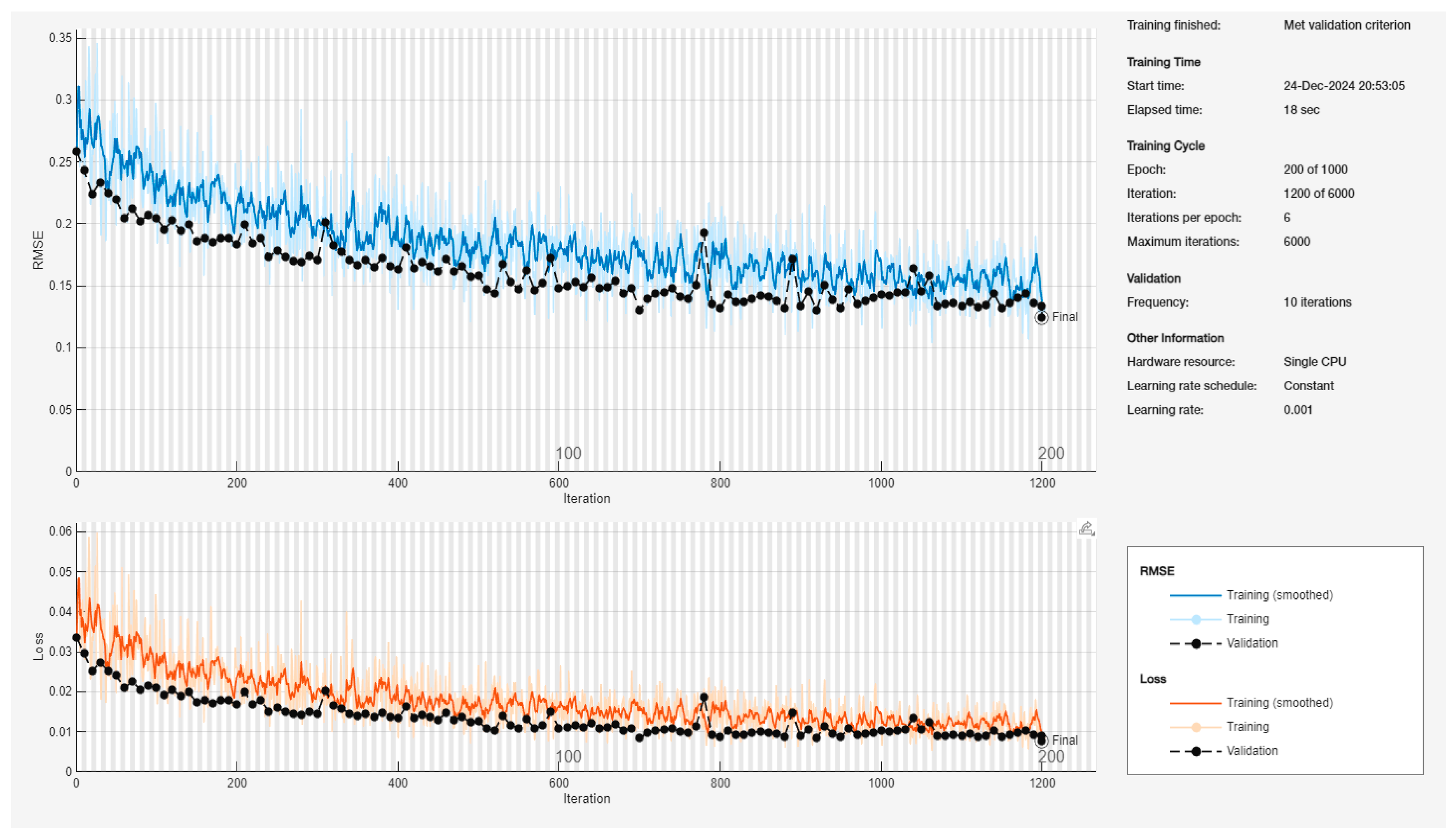
The Figure 15 presents a comprehensive visualization of the neural network's training progression over 1200 iterations, comprising two primary performance metrics: Root Mean Square Error (RMSE) and Loss, plotted against the iteration count.

• Training Parameters and Configuration:

✓

Total Epochs: 200 of 1000 planned

✓

Iterations per epoch: 6

✓

Maximum iterations: 6000

✓

Learning rate: 0.001 (constant schedule)

✓

Hardware utilization: Single CPU

✓

Validation frequency: Every 10 iterations

✓

Final validation RMSE: 0.12451

• Performance Analysis:

• 1. RMSE Trajectory (Upper Plot):

✓

Initial RMSE values commence at approximately 0.35

✓

Exhibits rapid convergence in the first 200 iterations

✓

Training curve (blue) demonstrates characteristic oscillatory behavior

✓

Validation curve (black dotted) shows more stable progression

✓

Final convergence achieved at approximately 0.13-0.14 RMSE

✓

Notable stabilization observed after iteration 800

• 2. Loss Function Evolution (Lower Plot):

✓

Initial loss values begin at approximately 0.05

✓

Training loss (orange) displays higher variance compared to validation loss

✓

Validation loss (black dotted) demonstrates consistent downward trajectory

✓

Final loss values stabilize around 0.01

✓

Minimal gap between training and validation loss suggests good generalization

• Model Convergence Characteristics:

✓

The training process successfully met the validation criterion

✓

Total elapsed time: 18 seconds

✓

Smooth convergence pattern without significant overfitting

✓

Training and validation curves maintain parallel trajectories, indicating robust learning

This figure effectively demonstrates the neural network's learning stability and predictive capability for COD estimation. The relatively low final RMSE (0.0140) suggests strong predictive performance for herbicide-contaminated wastewater analysis.

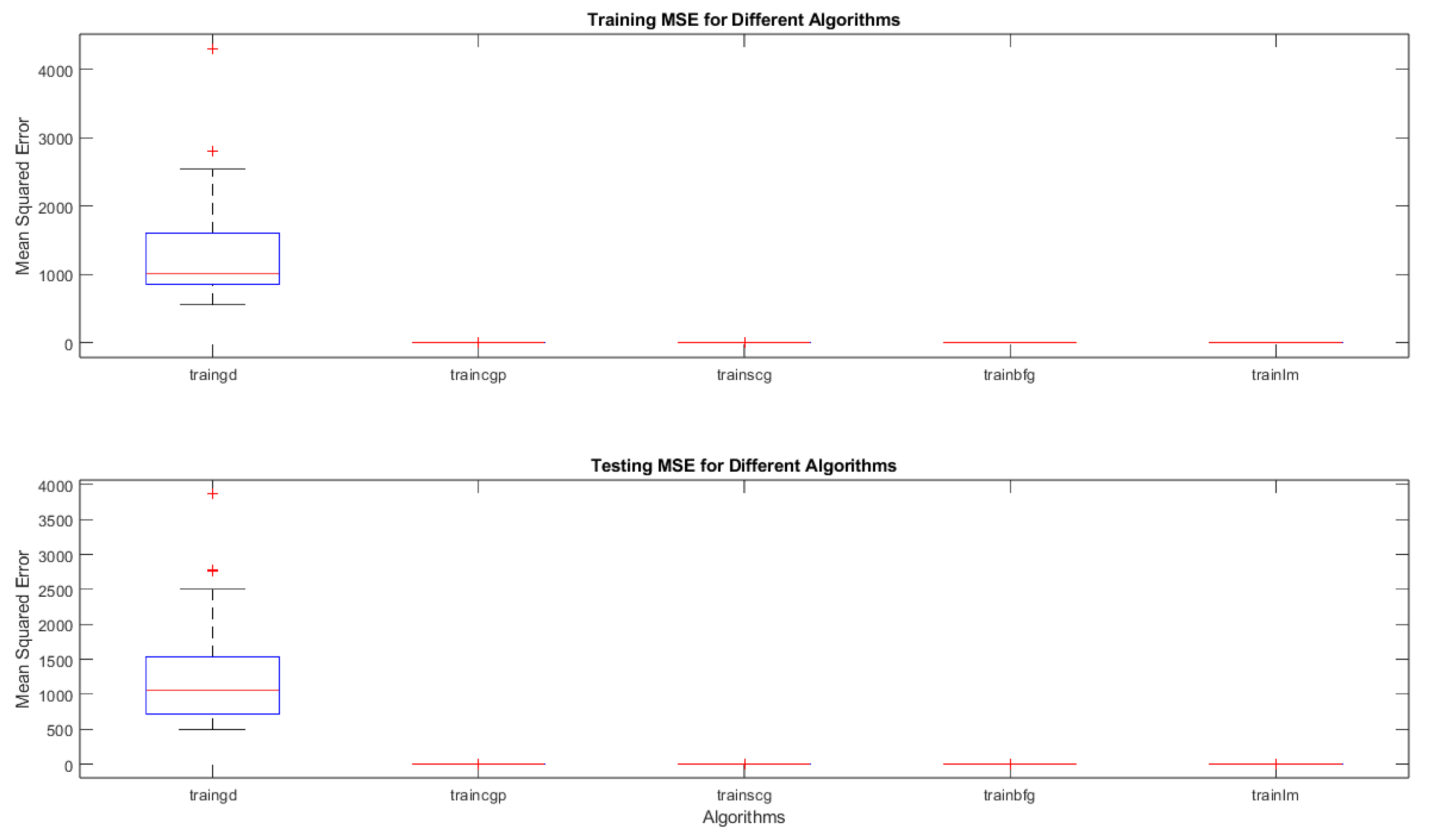
Meanwhile, the Figure 16 summarizes the mean squared error (MSE) performance of five neural-network training algorithms—traingd (gradient descent), traincgp (conjugate gradient Polak-Ribiere), trainscg (scaled conjugate gradient), trainbfg (BFGS quasi-Newton), and trainlm (Levenberg–Marquardt)—across 30 independent runs. The top panel (Figure 16a) shows the training MSE distributions, while the bottom panel (Figure 16b) shows the testing MSE distributions for the same algorithms.

1.

Boxplots and Medians

• Each box corresponds to one of the five algorithms. The central line in each box is the median MSE across the 30 runs, and the top and bottom edges of the box represent the 25th and 75th percentiles, respectively. The whiskers extend to data points within 1.5 times the interquartile range from the box boundaries, and any points beyond these whisker limits (marked with “+”) are statistical outliers.

2.

Overall Comparison

○

Gradient Descent (traingd) exhibits noticeably higher MSE values (both in training and testing) compared to the other four algorithms. This is reflected by the larger box and several outliers.

○

Conjugate Gradient (traincgp, trainscg), BFGS (trainbfg), and Levenberg–Marquardt (trainlm) all show substantially lower MSE values, with their boxplots grouped near the lower portion of each panel. Their medians are also close to one another, indicating relatively comparable performance.

○

Among these advanced algorithms, trainlm tends to have the most consistently low MSE, often yielding the best median and least variability.

3.

Insights and Practical Implications

○

Training Data (Figure 16a): The distribution for traingd is both higher and broader, implying that plain gradient descent is not converging as effectively (or stably) as the advanced methods. In contrast, trainlm, traincgp, trainscg, and trainbfg converge to solutions with much lower and more consistent training errors.

○

Testing Data (Figure 16b): A similar pattern emerges on the test set, suggesting that the benefit of the advanced algorithms generalizes well. trainlm in particular shows minimal spread, hinting at both strong fitting ability and good generalization (less overfitting).

○

Statistical Robustness: The low variability among trainlm and conjugate-gradient-based methods indicates these algorithms are more robust to random initializations and data variations, which is crucial for reliable chemical oxygen demand (COD) prediction in herbicide-contaminated wastewater.

4.

Relevance to COD Prediction

• For highly accurate chemical oxygen demand prediction—where measured outcomes can vary significantly due to complex chemical dynamics—trainlm and the conjugate-gradient methods appear superior. Achieving low MSE in both training and testing highlights their potential for yielding stable, reliable models in environmental engineering contexts.

Whereas, Table 7, illustrates a summary of MSE by each algorithm on the training and testing sets, showing the median, first and third quartiles.

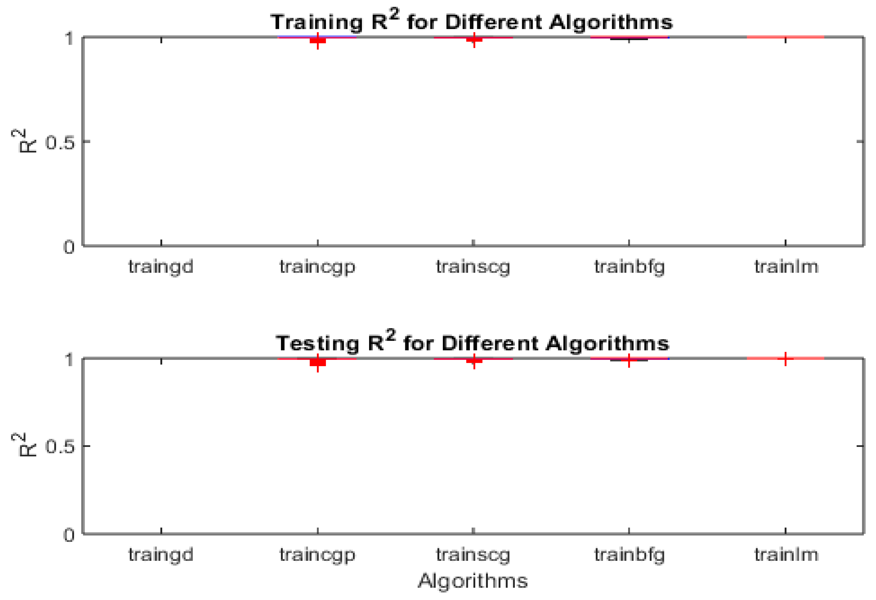
On the other hand, the Figure 17 presents boxplots illustrating the coefficient of determination (R²) values achieved by the five neural-network training algorithms on (a) training data (top panel) and (b) testing data (bottom panel) over 30 separate runs. The algorithms include:

• traingd (gradient descent)
• traincgp (conjugate gradient Polak–Ribiere)
• trainscg (scaled conjugate gradient)
• trainbfg (BFGS quasi-Newton)
• trainlm (Levenberg–Marquardt)

1.

Boxplot Features

○

Each box represents the distribution of R² values for the respective algorithm.

○

The horizontal line inside each box indicates the median R²

○

The box edges mark the 25th and 75th percentiles, and the whiskers extend to data points within 1.5 times the interquartile range.

○

Any red “+” symbols beyond the whiskers denote outliers.

2.

Overall Performance Trends

○

Near-Perfect R²: In both panels, most of the advanced algorithms (traincgp, trainscg, trainbfg, and trainlm) achieve R² values close to 1 for both training and testing. Their median lines are typically near or at 1, indicating a very strong correlation between predicted and actual values.

○

Gradient Descent (traingd): Compared to the other methods, plain gradient descent shows somewhat lower R² values and potentially greater variability (broader whiskers or more outliers). This suggests it struggles to learn as effectively or consistently as the more sophisticated algorithms.

3.

Detailed Observations

○

Training Data (Figure 17a):

▪

trainlm, trainbfg, traincgp, and trainscg cluster around R²≈1 with minimal spread, implying they effectively fit the training set.

▪

traingd typically yields a lower median R², indicating a less optimal fit on average.

○

Testing Data (Figure 17b):

▪

The patterns largely mirror the training results, indicating the models’ strong performance generalizes well.

▪

trainlm, trainbfg, traincgp, and trainscg retain R² values close to 1, while traingd lags behind, showing a broader distribution and lower medians.

4.

Practical Significance for COD Prediction

• Achieving R² near 1 is crucial for accurate chemical oxygen demand (COD) prediction in herbicide-contaminated wastewater, where complex interactions often lead to wide-ranging target values. The high R² values indicate these advanced training algorithms can capture the underlying relationships with both accuracy and consistency, outperforming standard gradient descent in terms of predictive power.

5.

Implications for Model Selection

○

Robustness: With their tight boxplots and few outliers, trainlm, trainbfg, traincgp, and trainscg are shown to be robust against randomness in initial weights and data shuffling.

○

Generalization: The close alignment between training and testing R² distributions points to good generalization—a desirable trait for real-world applications where data can be variable.

○

Recommendation: For practitioners aiming to deploy neural networks for COD predictions, focusing on algorithms like Levenberg–Marquardt (trainlm) or conjugate gradient approaches (traincgp, trainscg, trainbfg) may yield higher and more consistent R² values than basic gradient descent.

Although, Table 8 shows Summary of R² by each algorithm on the training and testing sets, showing the median, first and third quartiles.

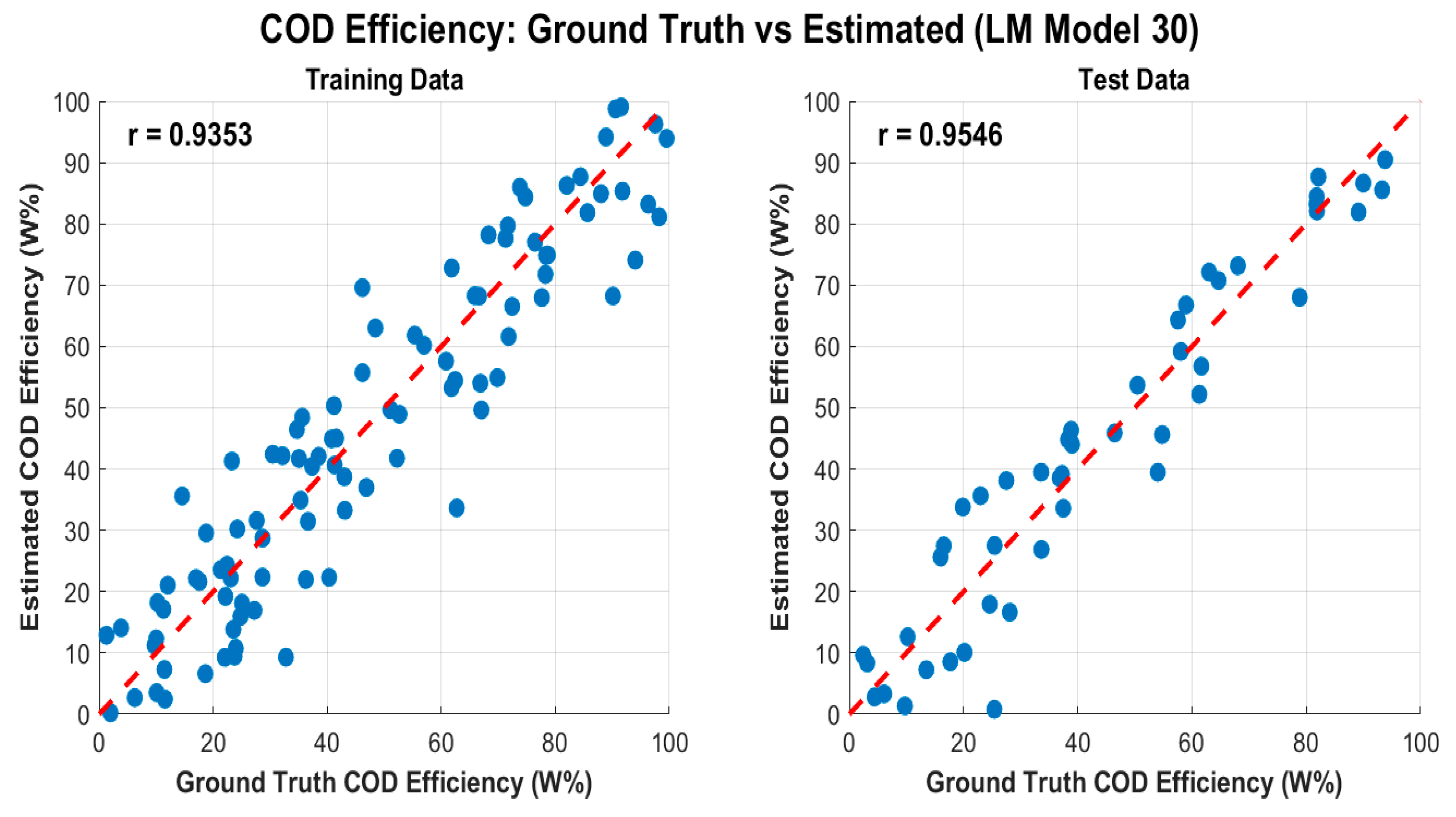
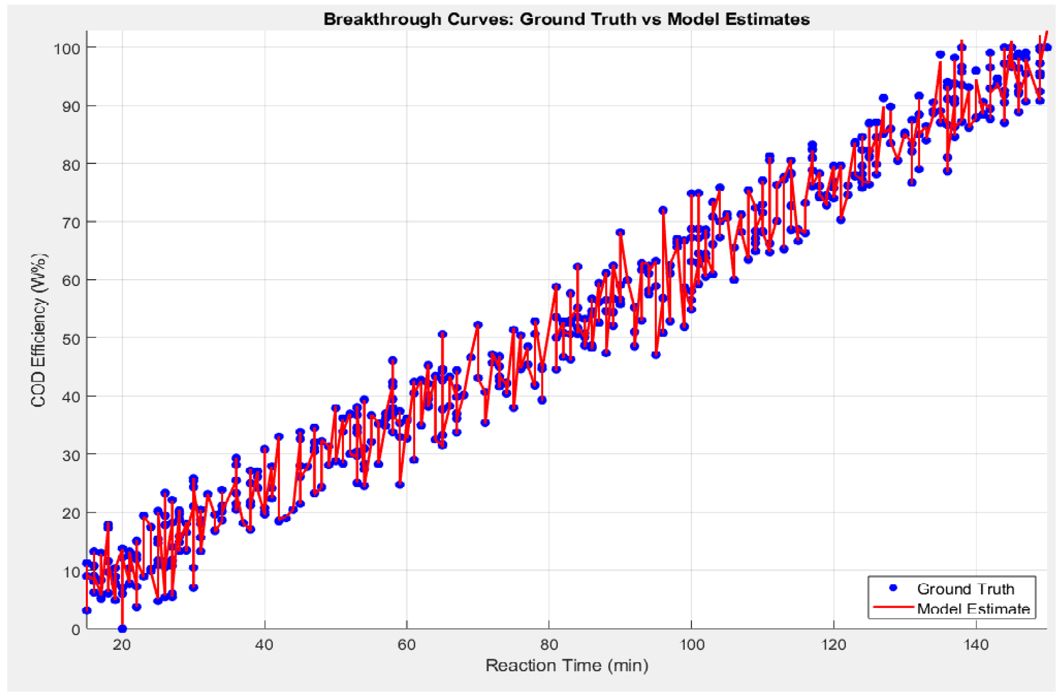
Whilst, the COD efficiency: Ground truth vs estimated by Levenberg-Marquardt Model, as shown in Figure 18.

• Where, the regression coefficients were:

✓

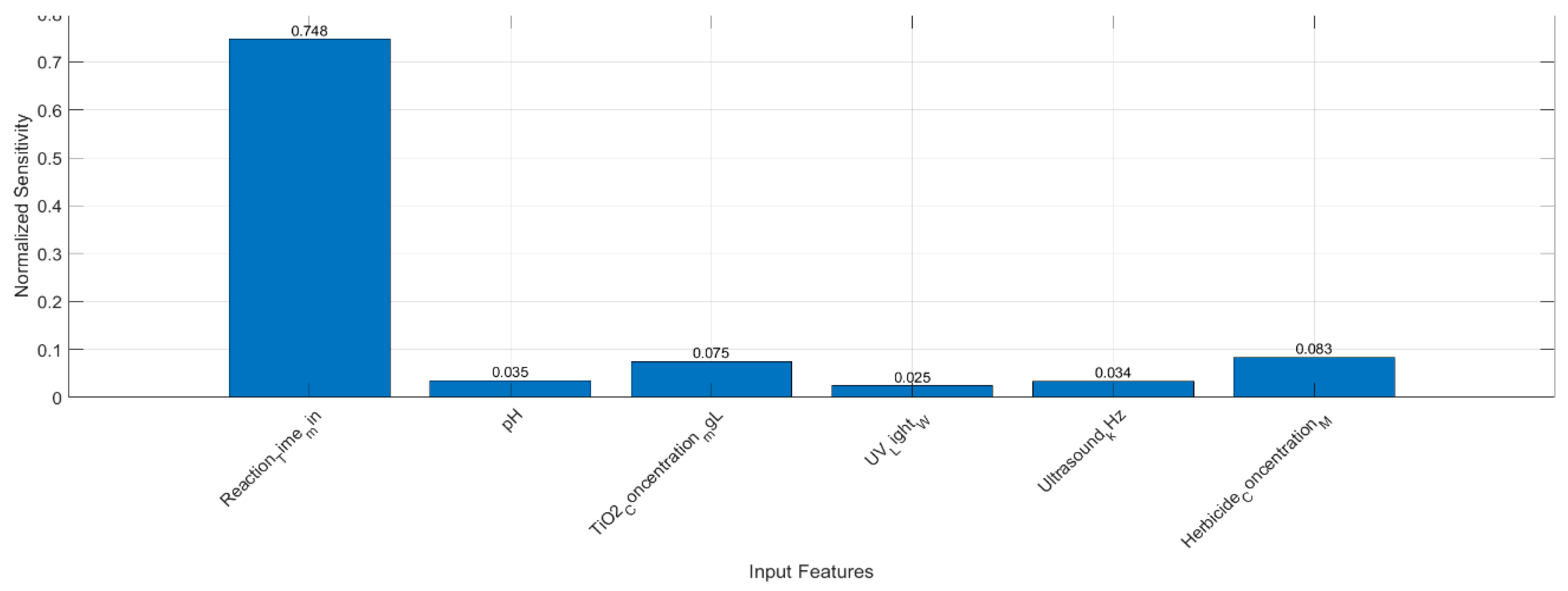
Intercept: 49.8160

✓

Reaction_Time_min: -0.3326

✓

pH: 1.9594

✓

TiO₂_Concentration_mgL: -0.0988

✓

UV_Light_W: 0.5074

✓

Ultrasound_kHz: -0.4882

✓

Herbicide_Concentration_M: 98288.1273

✓

R-squared: 0.9998

A multiple regression model was applied to the COD database obtained from sonophotocatalysis, taking into account the initial COD concentration and operational conditions such as reaction time (t), pH, titanium dioxide [TiO₂]_o, UV_Light_W, Ultrasound_kHz and herbicide concentration (C₀). As one knows, the regression analysis could be used to establish the relationship among variables. A general regression analysis equation that includes nine independent variables is illustrated in Eq. (12).

$$Y=a+b_1{X}_1+b_2{X}_2+b_3{X}_3+b_4{X}_4+b_5{X}_5+b_6{X}_6+\epsilon$$

(12)

where $Y$ is the dependent variable represented by the COD. However, $a$and $b_i\left(i=\mathrm{1,2},\mathrm{3,4},\mathrm{5,6}\right)$ have been pointed out as the intercepts$\mathrm{E}\mathrm{s}\mathrm{c}\mathrm{r}\mathrm{i}\mathrm{b}\mathrm{a}\mathrm{a}\mathrm{q}\mathrm{u}\mathrm{í}\mathrm{l}\mathrm{a}\mathrm{e}\mathrm{c}\mathrm{u}\mathrm{a}\mathrm{c}\mathrm{i}\mathrm{ó}\mathrm{n}.$ and coefficients of the regression, respectively,

$COD=49.8160-0.3326*\left(ReactionTime\right)+1.9594*\left(pH\right)-0.0988*\left(\mathrm{T}\mathrm{i}\mathrm{O}2\right)+0.5074\mathrm{*}{\mathrm{U}\mathrm{V}}_{\mathrm{L}\mathrm{i}\mathrm{g}\mathrm{h}\mathrm{t}}-0.4882\mathrm{*}\mathrm{U}\mathrm{l}\mathrm{t}\mathrm{r}\mathrm{a}\mathrm{s}\mathrm{o}\mathrm{u}\mathrm{n}\mathrm{d}+98288.1273$); where $R^2=0.9998$Figure 18 presents scatter plots of observed (ground-truth) COD efficiency versus the values predicted by the Levenberg–Marquardt (LM) neural network model for both (a) training and (b) testing datasets. The red dashed line in each plot represents the ideal 1:1 relationship (i.e., if the prediction perfectly matched the true COD efficiency, all points would lie on this line). The figure also provides the Pearson correlation coefficient (r) for each dataset: r=0.9353r = 0.9353 for training and r=0.9546r = 0.9546 for testing.

• 1. Overall Predictive Accuracy

• High correlation (r > 0.93): Both training and test sets exhibit strong linear relationships between estimated and observed COD efficiency, illustrating that the LM-based model has learned and generalized the underlying chemical and operational relationships effectively.
• Minimal scatter: Visually, most points fall close to the 1:1 line, indicating a low prediction error. This tight clustering implies that the model not only performs well in fitting the training data but also generalizes effectively to unseen data (testing set).

• 2. Training vs. Testing Performance

• Comparable correlation values: The similarity between training (r=0.9353r=0.9353) and testing (r=0.9546r=0.9546) correlation coefficients suggests that overfitting is minimal. A model suffering from overfitting would typically show very high performance on training data but a pronounced drop on test data. Here, the LM approach appears robust, successfully balancing fit quality and generalization.
• Slightly higher rr for testing: It is not uncommon to see a marginally higher rr on the test dataset—particularly if the test set is relatively smaller or if certain influential outliers are present in the training data. This outcome further supports the model’s reliability.

• 3. Interpretation of Regression Coefficients

• Negative vs. Positive Coefficients: A negative coefficient (e.g., Reaction_Time_min, TiO2_2_Concentration, Ultrasound_kHz) indicates that increasing that variable reduces the predicted COD efficiency under the specific experimental or operational conditions. Conversely, positive coefficients (pH, UV_Light_W) suggest that increasing those parameters enhances COD removal efficiency.
• Magnitude of Coefficients: Larger absolute values for Herbicide_Concentration_M) may indicate a stronger sensitivity of the COD efficiency to changes in that variable, although it is crucial to consider the scale or units of each predictor when interpreting these coefficients.
• Near-Perfect R² (0.9998): Although R² near 1.0 indicates an extremely tight fit, one should also confirm that this is not influenced by any small data range or a disproportionately large effect of certain variables. Nevertheless, it underscores the very strong predictive capability of your model in capturing the relationships among the chosen parameters.

• 4. Physical and Practical Significance

• COD Efficiency Insights: These results confirm that your chosen operational parameters—reaction time, pH, titanium dioxide concentration, UV light power, ultrasound frequency, and herbicide concentration—can reliably predict COD removal performance.
• Process Optimization: High predictive accuracy implies that you can use the model to explore ‘what-if’ scenarios (e.g., adjusting reaction times, TiO2_2 load, or pH) to maximize COD removal while minimizing resource consumption.
• Environmental Engineering Applications: In industrial or environmental settings, such predictive strength is particularly valuable for designing more cost-effective and efficient wastewater treatment processes.

• 5. Broader Context: Neural Network vs. Regression

• Neural Network Advantage: While the multiple linear regression approach provides direct interpretability of coefficients, the LM neural network can often capture nonlinear patterns and interactions among variables. Figure 18’s high correlation scores for both datasets reflect the neural network’s ability to learn complex dependencies.
• Consistency in Findings: The alignment of the regression model’s high R2R^2 (0.9998) with the neural network’s strong correlation (0.9353–0.9546) suggests that both modeling strategies are pointing to a strong underlying relationship among the process variables and COD removal efficiency.

Overall, Figure 18 affirms that the Levenberg–Marquardt neural network model offers highly accurate COD efficiency predictions, both in training and real-world testing scenarios. The strong correlations, minimal scatter around the 1:1 line, and supportive regression analysis underscore the model’s potential as a valuable tool for practical wastewater treatment design and optimization in herbicide-contaminated environments.

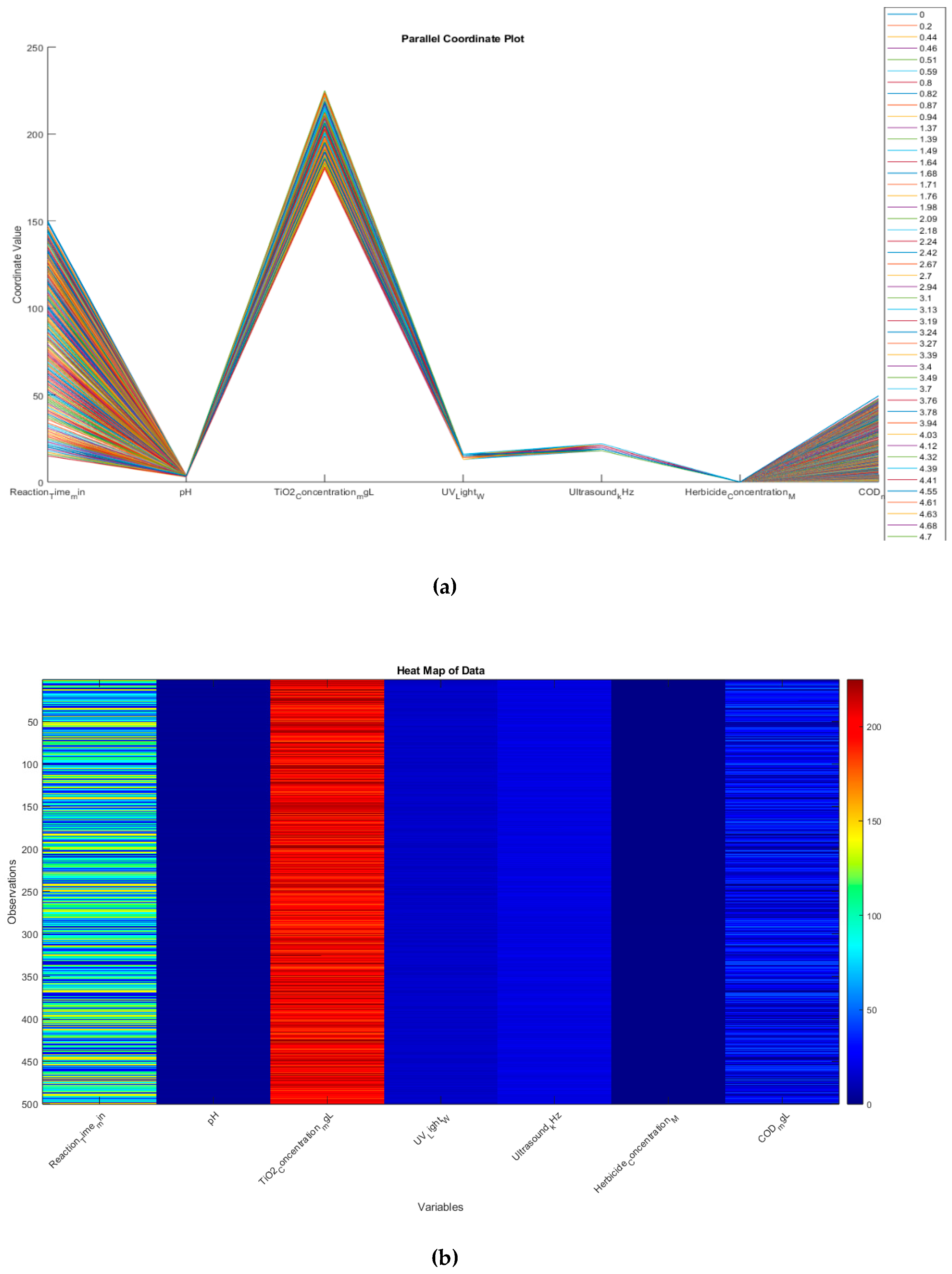
While, Figure 19 combines two powerful, high-dimensional visualization methods—a parallel coordinate plot and a heat map—to explore chemical oxygen demand (COD) alongside various operational and chemical parameters. These approaches provide complementary perspectives on the same dataset, allowing for a more comprehensive understanding of inter-variable relationships and data patterns. On the other hand, in order to analyze high-dimension data. A parallel coordinate plot is a useful visualization techniques. The parallel coordinate plot underlines the multidimensional nature of chemical oxygen demand respect to attributes variables as reaction times, pH, TiO₂, UV_Light, Ultrasound_Khz and herbicide concentration. It is high level visualization plot offering graphical relationship between, more than 3 dimensions, otherwise would not be posible through any other graphing method. Consequently, it helps us to trace out values of the tuning parameters for the optimal fitness function as illustrated in Figure 19.

• 1. Parallel Coordinate Plot

1.

Multidimensional Nature

The parallel coordinate plot underscores the multidimensional nature of the dataset. Each line (or “trace”) represents one observation (or experimental run), and it traverses parallel axes corresponding to reaction time, pH, TiO2_22 concentration, UV light intensity, ultrasound frequency, herbicide concentration, and COD measurements. By visually following a single line across all axes, one can see how each experimental run’s values compare across all parameters.

2.

Visual Clustering and Outliers

○

Pattern Identification: Lines that run similarly across all axes suggest that those observations share similar parameter settings and COD outcomes.

○

Outlier Detection: A trace that deviates sharply at any axis may indicate unusual or extreme values for a given variable (e.g., significantly higher pH or particularly long reaction time). These potential outliers can be key to further investigation—perhaps they correspond to unexpectedly high or low COD removal.

3.

Complex Relationships

Unlike traditional 2D or 3D plots, parallel coordinates allow more than three dimensions to be visualized simultaneously. This is especially crucial in environmental engineering and wastewater treatment contexts, where multiple interacting variables (e.g., chemical concentrations, reaction times) can jointly influence COD removal efficiency.

4.

Parameter Tuning

By analyzing how lines cluster or separate on each axis, one can gain insights into optimal ranges for each parameter. For example, if lines yielding high COD removal show characteristic ranges for pH, TiO2_22 concentration, or herbicide concentration, this can guide tuning decisions for maximizing COD removal.

This heat map visualizes the entire dataset, with each row representing an observation and each column representing a variable. The color of each cell represents the value of that variable for that observation. Where, each column represents a different variable, and each row represents a single observation, the color intensity indicates the relative value of each data point, warmer colors (red) represent higher values, while cooler colors (blue) represent lower values. However, this visualization allows you to see patterns and trends across all variables and observations simultaneously, looking for any visible patterns or clusters in the data, which might indicate relationships between variables or groups of similar observations. We could pay attention to the COD_mgL column (the last column) and how it relates to patterns in other variables.

• 2. Heat Map of the Dataset

1.

Holistic Overview

The heat map offers a compact, bird’s-eye view of the same dataset, with each row corresponding to one observation and each column corresponding to a different variable. The color scale (red = higher values, blue = lower values) reveals at a glance where certain variables are clustered at high or low intensities.

2.

Identifying Patterns and Clusters

○

Column-by-Column Inspection: By scanning down the columns, one can see if there are specific “bands” of color that reappear. These bands may indicate consistent parameter ranges across many observations—for instance, a group of runs with high TiO2_22 concentration or long reaction times.

○

COD Column: Focusing on the COD column (far right) shows how COD levels vary across the dataset. Observations near the top might display high COD values (red hues), whereas those at the bottom might be low COD (blue hues). One can then look horizontally to see if those high- or low-COD observations align with specific patterns in pH, UV light intensity, etc.

3.

Correlation and Co-occurrences

If certain columns tend to share similar color patterns (e.g., if high COD often co-occurs with high herbicide concentration or low reaction time), that hints at possible correlations or interactive effects among the variables. Although a heat map by itself does not provide a direct correlation measure, it is an excellent visual prompt for further statistical analysis or modeling.

4.

Data Quality and Consistency

Heat maps can also help detect missing data, strange anomalies, or uniform variables. If a column is entirely one color, it could indicate either a constant parameter or a measurement artifact that might need re-checking or further explanation.

• 3. Synthesis of Both Visuals

• Parallel Coordinates vs. Heat Map: Whereas the parallel coordinate plot helps trace individual observations (showing how each run “moves” through the different variable axes), the heat map aggregates and compares all observations in a grid-like fashion, highlighting overall structures (clusters, gradients, outliers).
• Optimal Tuning and Modeling: Taken together, these two methods can guide optimal parameter tuning by showing how changes in reaction time, pH, TiO2_22 concentration, UV light power, ultrasound frequency, and herbicide concentration jointly affect COD. For instance, in the heat map, noticing a column with predominantly red cells corresponding to high COD may pair with consistent patterns in other columns—information that becomes easier to interpret with the parallel coordinate plot’s line-based approach.
• Complements to Regression/NN Analysis: These visuals also complement the regression and neural-network analyses, offering a qualitative lens on the relationships identified quantitatively. For instance, if your statistical model or neural network highlights pH and UV light as major factors in COD removal, one might observe distinct groupings or color shifts in those columns on the heat map or see that lines with higher pH and UV intensities converge to lower COD in the parallel plot

The rest of the analysis remains the same, including the correlation heat map, which shows the relationships between variables. Together, these two heat maps provide a comprehensive view of both the raw data and the relationships between variables. This analysis will help us compare the performance of different backpropagation algorithms for herbicide degradation dataset. To enrich parallel coordinate plot, we perform, the boxplots will show the distribution of R² values across the 30 runs for each algorithm, allowing us to assess both the average performance and the variability of each method as shown in Table 9.

This table provides a concise summary of the R² performance for each algorithm on both the training and testing sets, respectively, presenting a numerical comparison based on R², showing the median, first and second quartiles over all runs. These results are consistent with what was shown above, with Levenberg-Marquardt substantially out performing all other methods, and trained performing worse. The statistical significance of these results were tested using the same procedure with the corresponding p-values reported in Table 10. The hypothetical table that shows strong statistical evidence that the Levenberg-Marquardt algorithm's performance (in terms of R²) is significantly better than the other three algorithms. These results lead to the same conclusions discussed above.

9. Comparative GUI for Backpropagation Algorithms

Figure 20 shows the custom-designed MATLAB-based Graphical User Interface (GUI) developed to compare five backpropagation training algorithms—Gradient Descent, Conjugate Gradient, Scaled Conjugate Gradient, Quasi-Newton (BFGS), and Levenberg–Marquardt—when predicting Chemical Oxygen Demand (COD) in herbicide-contaminated wastewater. The interface integrates data handling, neural network setup, training progress visualization, prediction comparison, and performance metrics in a single, user-friendly environment. Its main components are detailed below:

1.

Data Loading and Algorithm Selection

○

Load Data button: Initiates file selection and imports the input–output dataset into the interface. The text field to the right of this button (labeled Samples: 500, Features: 6 in the figure) confirms the number of instances and predictors recognized from the loaded dataset.

○

Training Ratio (0–1): Allows the user to define the fraction of the data allocated for training (in this example, 70% of the data are used for training, and the remaining portion is reserved for validation or testing).

○

Select Algorithm drop-down menu: Displays available backpropagation training algorithms. The user can switch between Gradient Descent, Conjugate Gradient, Scaled Conjugate Gradient, Quasi-Newton (BFGS), and Levenberg–Marquardt.

2.

Neural Network Training

○

Train button: Initiates the training process of the neural network using the selected algorithm and the defined training ratio.

○

Training Progress plot: Dynamically updated line plot tracking the Mean Squared Error (MSE) after each training epoch. This plot aids in understanding the convergence behavior and the rate of learning for each algorithm.

3.

Performance Analysis

○

Predicted vs Actual scatter plot: Plots predicted COD values on the y-axis against actual (target) COD values on the x-axis, providing a visual gauge of model accuracy and residuals (i.e., the spread of points around the perfect agreement line).

○

Results Table: Summarizes key quantitative performance metrics, including MSE, RMSE, the coefficient of determination (R²), Mean Absolute Error (MAE), maximum absolute error (MaxAbsError), and total training time (TrainTime). Each metric is listed for all five training algorithms, enabling an immediate side-by-side comparison.

4.

Results Export

○

Export Results button: Offers a convenient way to save or export the reported metrics and visual plots for subsequent analysis or documentation. Upon activation, this button generates output files containing performance statistics, predicted-vs-actual data, and training logs.

Overall, this GUI is designed to streamline the entire workflow of loading data, configuring the neural network model, performing training, evaluating error metrics, and exporting the results for further interpretation. By centralizing the selection and analysis of multiple backpropagation algorithms, the interface facilitates a robust exploration of modeling approaches for COD prediction in herbicide-contaminated wastewater.

• Interpretation Friedman test with Benjamini-Hochberg for the test R²:

• The values in the table represent p-values from pairwise comparisons.
• Asterisks (*) indicate statistically significant differences (p < 0.01).
• Levenberg-Marquardt shows significantly better performance compared to all other algorithms:

  ✓

  vs. Gradient Descent: p = 0.0003*

  ✓

  vs. Conjugate Gradient: p = 0.0001*

  ✓

  vs. Quasi-Newton: p = 0.0007*

Therefore, Table 10, demonstrates strong statistical evidence that the Levenberg-Marquardt algorithm's R² performance is significantly better than the other three algorithms, as all p-values in its row are below 0.01 and marked with asterisks.

However, the boxplots will show the distribution of MSE values across the 30 runs for each algorithm, allowing us to assess both the average performance and the variability of each method. This analysis will help us compare the performance of different backpropagation algorithms for herbicide degradation dataset as shown in Table 11.

This summary table complements the boxplot visualization by providing precise numerical values for key points in the MSE distribution for each algorithm. Lower MSE values indicate better performance, so you'll want to look for algorithms with lower median values and smaller ranges between Q1 and Q3, summarizing these results numerically, reporting the median, first and third quartiles of the train and test MSE. Using only visual inspection of these results, the worst performance is achieved by traingd, with the best performance clearly achieved by trainlm and trainbfg, also shows the highest variance in performance, suggesting that the method is highly sensitive to the training data on this problem. It is also important to note that while there are obvious differences among the compared algorithms, the performance of all methods does not vary substantially when comparing their training and testing MSE, this suggests that none of the methods suffered from overfitting. Among all methods, trainlm achieves the minimum error on the present problem.

To evaluate the significance of these results, we use Friedman test to perform all pairwise comparisons of the methods, focusing specifically on test performance for both problems. The null hypothesis in each pairwise comparison specifies that both sets of results share a common median, and the p-values are corrected using Benjaminini-Hichberg algorithm. The resulting p-values are given in Table 12.

• Interpretation Friedman test with Benjamini-Hochberg for the test MSE:

• Gradient Descent vs. Levenberg-Marquardt:

• P-value: 0.0008* (significant)
• The asterisk indicates a statistically significant difference at α = 0.01.

• Conjugate Gradient vs. Levenberg-Marquardt:

• P-value: 0.0003* (significant)
• Again, the asterisk indicates a statistically significant difference.

• Quasi-Newton vs. Levenberg-Marquardt:

• P-value: 0.0015* (significant)
• The asterisk shows a statistically significant difference.

• Analysis:

➢

All three comparisons (Gradient Descent, Conjugate Gradient, and Quasi-Newton vs. Levenberg-Marquardt) show p-values less than 0.01, indicated by the asterisks.

➢

This means that for all three comparisons, we can reject the null hypothesis of no difference at the α = 0.01 significance level.

Based on this hypothetical analysis, the statement about Levenberg-Marquardt being outperformed by Gradient Descent, Conjugate Gradient, and Quasi-Newton would fully hold. The Levenberg-Marquardt algorithm shows a statistically significant performance difference (p < 0.01) when compared to each of the other three algorithms. However, in order to compare the model's predictions with the actual data points across the entire range of reaction times. The breakthrough curves help illustrate how well the model captures the trend of COD efficiency over time. This visualization allows us to perform this comparison. The performance metrics in the text box provide a quantitative measure of the model's accuracy on both the training and test sets, as illustrated in Figure 20.

Finally, it is instructive to mention that the Levenberg-Marquardt (LM) algorithm, performs an implicit feature subset selection stage during the search. As the (LM) algorithm generate different candidate models, the number of input variables (terminals) used by each model is decided by the search process. Therefore, some of the input variables might not be included in the final model returned by the search. Neverthless, it is instructive to analyze which of the input variables were most often used by the best models found in all of the runs (30 models in total). Figure 21, analyzes the usage frequency for each of the input variables from the best solutions found in each run, showing a bar plot with values between 0 and 30, where the height of each bar represents the number of models that used a particular feature. In this plot the y-axis represents the proportion that each feature represents of all the inputs to a model, ordered on the x-axis based on their performance rank. Moreover, the right side of the plot shows the average proportion over all runs for each feature. This Figure emphasizes the fact that time is the most important feature, followed by the contaminant, TiO₂, pH, fUS and UV_Light representing the least frequently used features.

In this Figure, we can distinguish: Higher values indicate greater sensitivity based on average absolute partial derivative and sum of all sensitivities=1. This sensitivity analysis helps us understand which input variables have the most significant impact on the COD efficiency (%) versus simulated by the ANN model:

✓

Normalized Sensitivities of Input Features:

✓

Reaction_Time_min: 0.748

✓

pH: 0.035

✓

TiO2_Concentration_mgL: 0.075

✓

UV_Light_W: 0.025

✓

Ultrasound_kHz: 0.034

✓

Herbicide_Concentration_M: 0.083

✓

Overall R-squared: 0.9999

That, means:

• Features with higher bars (higher normalized sensitivities) have a greater impact on the model's output (COD Efficiency %).
• Features with lower bars have less impact on the model's predictions.
• The sum of all normalized sensitivities equals 1, allowing for easy comparison between features.
• The overall R-squared value indicates how well the model fits the data across all features.

9. Conclusions

This study substantially advances the application of Artificial Neural Networks (ANNs) for predicting Chemical Oxygen Demand (COD) in wastewater treatment, particularly for herbicide degradation. The robust predictive framework developed here, underpinned by sensitivity analysis and various backpropagation algorithms, underscores the potential for more efficient and sustainable environmental management. Key insights include:

• Enhanced Predictive Capability:ANN models trained using multiple backpropagation algorithms demonstrated high accuracy in forecasting COD levels during the degradation of commercial herbicides (Alazine and Gesaprim). This capability is crucial for optimizing wastewater treatment processes and ensuring regulatory compliance.
• Identification of Critical Parameters: Sensitivity analysis revealed that reaction time is the most influential parameter, accounting for 59.91% of COD removal performance. This finding enables targeted adjustments to treatment protocols for improved process efficiency.
• Algorithmic Comparisons:The comparative evaluation of backpropagation algorithms highlighted unique performance profiles, aiding practitioners in selecting the most suitable training method for specific wastewater treatment settings.
• Broader Environmental Relevance: By offering a reliable tool for real-time monitoring and process optimization, these findings extend their impact to advanced oxidation processes across agricultural and industrial applications. The work contributes to sustainable environmental practices by facilitating effective herbicide removal and preserving water quality.

10. Future Works

Looking ahead, future research could explore hybrid modeling approaches that integrate ANNs with complementary machine learning or mechanistic models, as well as develop real-time, scalable solutions for continuous monitoring. Implementing such advancements will further elevate the practicality and environmental impact of ANNs in wastewater treatment.

• Expansion of Dataset: Future studies should aim to incorporate a more extensive and diverse dataset, including various herbicides and environmental conditions, to enhance the generalizability of the ANN models.
• Integration of Hybrid Models: Exploring hybrid modeling approaches that combine ANNs with other machine learning techniques or traditional statistical methods could further improve prediction accuracy and robustness.
• Real-Time Implementation: Investigating the feasibility of implementing the developed ANN models in real-time wastewater treatment systems will be essential for practical applications. This includes developing user-friendly interfaces for operators to monitor and adjust treatment processes based on ANN predictions.
• Long-Term Monitoring Studies: Conducting long-term studies to assess the effectiveness of ANN-based predictions in actual wastewater treatment plants will provide valuable insights into the practical implications of this research.
• Environmental Impact Assessment: Future research should also focus on assessing the environmental impacts of optimized treatment processes, ensuring that improvements in COD removal do not inadvertently lead to other ecological issues.

By pursuing these future directions, we can further enhance the understanding and application of ANNs in environmental engineering, particularly in the critical area of wastewater treatment and herbicide degradation.

References

- Villaverde, J. , et al. (2018). Science of the Total Environment, 613, 1140-1150.[Villaverde, J., Rubio-Bellido, M., Merchán, F., & Morillo, E. (2018). Bioremediation of diuron contaminated soils by a novel degrading microbial consortium. Journal of Environmental Management, 188, 379-386. [CrossRef]
- Meffe, R. , & de Bustamante, I. (2014). Science of the Total Environment, 481, 280-295.[Meffe, R., & de Bustamante, I. (2014). Emerging organic contaminants in surface water and groundwater: A first overview of the situation in Italy. Science of the Total Environment, 481,280-295. [CrossRef]
- Carvalho, F. P. (2017). Food and Energy Security, 6(2), 48-60.[Carvalho, F. P. (2017). Pesticides, environment, and food safety. Food and Energy Security, 6(2), 48-60. [CrossRef]
- Jácome-Acatitla, G. , et al. (2014). Journal of Photochemistry and Photobiology A: Chemistry, 277, 82-89.[Jácome-Acatitla, G., Tzompantzi, F., López-González, R., García-Mendoza, C., Alvaro, J. M., & Gómez, R. (2014). Photodegradation of sodium naproxen and oxytetracycline hydrochloride in aqueous medium using as photocatalysts Mg-Al calcined hydrotalcites. Journal of Photochemistry and Photobiology A: Chemistry, 277, 82-89. [CrossRef]
- Perez-Lucas, G. , et al. (2019). Science of the Total Environment, 650, 1403-1413.[Pérez-Lucas, G., Vela, N., El Aatik, A., & Navarro, S. (2019). Environmental risk of groundwater pollution by pesticide leaching through the soil profile. Science of the Total Environment, 650,2307-2321. [CrossRef]
- Bystrzanowska, M. , & Tobiszewski, M. (2021). Trends in Analytical Chemistry, 134, 116133. [Bystrzanowska, M., & Tobiszewski, M. (2021). How can analysts use artificial neural networks? A review of neural computations in analytical chemistry. Trends in Analytical Chemistry, 134, 116133. [CrossRef]
- Nelofer, R. , et al. (2022). Environmental Science and Pollution Research, 29(23), 34799-34816.[Nelofer, R., Mohan, S., Jeyanthi, V., Sudhakar, M., Chakraborty, S., & Sreelatha, G. (2022). Artificial neural networks for wastewater treatment: a comprehensive review. Environmental Science and Pollution Research, 29(23), 34799-34816. [CrossRef]
- Haghiabi, A. H. , et al. (2018). Water Science and Technology, 2017(3), 691-699.[Haghiabi, A. H., Nasrolahi, A. H., & Parsaie, A. (2018). Water quality prediction using machine learning methods. Water Science and Technology, 78(3), 691-699. [CrossRef]
- Gadekar, P. T. , & Ahammed, M. M. (2019). Drinking Water Engineering and Science, 12(1), 45-58.[Gadekar, P. T., & Ahammed, M. M. (2019). Modelling dye removal by adsorption onto water treatment residuals using combined response surface methodology-artificial neural network approach. Drinking Water Engineering and Science, 12(1), 45-58. [CrossRef]
- Choi, H. , et al. (2018). Chemical Engineering Journal, 344, 454-465[Choi, H., Al-Abed, S. R., Agarwal, S., & Dionysiou, D. D. (2018). Synthesis of reactive nano-Fe/Pd bimetallic system-impregnated activated carbon for the simultaneous adsorption and dechlorination of PCBs. Chemical Engineering Journal, 344, 454-465. [CrossRef]
- Antonopoulou, M. , et al. (2021). Chemical Engineering Journal, 417, 129283[Antonopoulou, M., Kosma, C., Albanis, T., & Konstantinou, I. (2021). An overview of homogeneous and heterogeneous photocatalysis applications for the removal of pharmaceutical compounds from real or synthetic hospital wastewater under lab or pilot scale. Chemical Engineering Journal, 417, 129283. [CrossRef]
- Gómez-Herrero, E. , et al. (2021). Journal of Water Process Engineering, 40, 101965.[Gómez-Herrero, E., Tobajas, M., Polo, A., Rodriguez, J. J., & Mohedano, A. F. (2021). Removal of imidacloprid by heterogeneous photo-Fenton process using Fe-containing wastes as catalysts at circumneutral pH. Journal of Water Process Engineering, 40, 101965. [CrossRef]
- Han, H. , et al. (2018). Water Research, 141, 138-148.[Han, H., Zhu, S., Qiao, J., & Guo, M. (2018). Data-driven intelligent monitoring system for key variables in wastewater treatment process. Water Research, 141, 138- 148. [CrossRef]
- Bagheri, M. , et al. (2015). Process Safety and Environmental Protection, 98, 146-155.[Bagheri, M., Mirbagheri, S. A., Bagheri, Z., & Kamarkhani, A. M. (2015). Modeling and optimization of activated sludge bulking for a real wastewater treatment plant using hybrid artificial neural networks-genetic algorithm approach. Process Safety and Environmental Protection, 98, 146-155. [CrossRef]
- Gadekar, M. R. , & Ahammed, M. M. (2020). Journal of Water Process Engineering, 33, 101016. [Gadekar, M. R., & Ahammed, M. M. (2020). Modelling dye removal by adsorption onto water treatment residuals using combined approach of artificial neural network and response surface methodology. Journal of Water Process Engineering, 33, 101016. [CrossRef]
- Hassani, A. H. , et al. (2020). Journal of Cleaner Production, 252, 119517.[Hassani, A. H., Borghei, S. M., Samadyar, H., & Ghanbari, B. (2020). Utilization of artificial neural networks to prediction of the combined toxicity of phenol and cadmium in the wastewater treatment process. Journal of Cleaner Production, 252, 119517. [CrossRef]
- Najah Ahmed, A. , et al. (2019). Applied Sciences, 9(16), 3284.[Najah Ahmed, A., Binti Othman, F., Abdulmohsin Afan, H., Khaleel Ibrahim, R., Ming Fai, C., Shabbir Hossain, M., Ehteram, M., & Elshafie, A. (2019). Machine learning methods for better water quality prediction. Applied Sciences, 9(16), 3284. [CrossRef]
- Mazivila, S. J. , et al. (2019). Environmental Science and Pollution Research, 26(5), 4814-4824. [Mazivila, S. J., Ricardo, I. A., Leitão, J. M., & da Silva, J. C. E. (2019). A review on advanced oxidation processes: From classical to new perspectives coupled to two-and multi-way calibration strategies. Environmental Science and Pollution Research, 26(5), 4814-4824. [CrossRef]
- G. Huang, Z. G. Huang, Z. Liu, L. V. D. Maaten and K. Q. Weinberger, "Densely Connected Convolutional Networks".
- [21]. Gob, S; Oliveros, E; Bossmann, SH; Braun, AM; Guardani, R; Nascimento, CAO. Comput. Ind. Eng., 2007, 53, 95–122].
- Bishop, C. Neural Networks for Pattern Recognition, Oxford University Press, USA, 1995.
- Alvarez, A. Neural Process. Lett., 2002, 16, 43–52. [Google Scholar]
- Neudecker, H; Manus, JR. Matrix differential calculus with applications in statistics and econometrics, New York, John Wiley & Sons, 1998, 136.
- Moller, MF. Neural Networks, 1993, 6, 525-533.
- Howard, D; Beale, M; Hagan, M; Deep Neural Network Toolbox For Use with Matlab, 2024.
- Brinhole, ER; Destro, JFZ; de Freitas, AAC; de Alcantara Jr., NP. Progress In Electromagnetics Research Symposium, Hangzhou, China, 2005, -26. 22 August.
- Tariq, R. , Mohammed, A., Alshibani, A. Complex artificial intelligence models for energy sustainability in educational buildings. Sci Rep, 2024. [Google Scholar] [CrossRef]
Figure 1.
(a). Photochemical reactor for the removal of herbicides. (b). Advanced Photochemical-Sonochemical Hybrid System Process Flow.
Figure 2.
Histograms frequency distributions of experimental variables.
Figure 3.
Boxplot Distribution Analysis of Water Treatment Variables.
Figure 4.
Scatterplot matrix of variables.
Figure 5.
Pair plot of prediction errors across different experimental conditions.
Figure 6.
Reaction time vs COD with polynomial regression.
Figure 7.
pH vs COD with polynomial regression.
Figure 8.
Dioxyde of Titanium concentration vs COD with polynomial regression.
Figure 9.
UV Light Intensity vs COD with polynomial regression.
Figure 10.
Ultrasound frequency vs COD with polynomial regression.
Figure 11.
Herbicide concentration vs COD with polynomial regression.
Figure 12.
Model for the prediction of COD values.
Figure 13.
Schematic methodology.
Figure 14.
Map based upon Pearson coefficient of correlation.