
Submitted:
14 June 2024
Posted:
17 June 2024
You are already at the latest version
Abstract
Modeling the reaction time required for the removal of chemical oxygen demand (COD) from wastewater is important because can be an indicator of harmful pollutants that may pose risks to human health.. Here, we evaluate the use of an inverse artificial neural network (ANNi) to optimize the removal of COD from aqueous herbicide solutions using sonophotocatalysis as the treatment process.. This algorithm takes the operating conditions as input and estimates the optimal reaction time to reach the required effluent COD. This model was validated by comparison with both experimental measurements and simulated analysis, resulting in low error (0.5%), high Pearson correlation (R2 = 0.9956), and short computing time (less than one minute). The results for the proposed methodology (ANNi-GAs) were efficient and attractive in a reasonable way providing a satisfactory picture of the relationships between the optimal input parameters. Such parameters control the degradation process of herbicides online and can be used to predict the behavior of COD removal, thus taking actions to reduce the impact of aqueous treatment with alazine and gesaprim herbicides on aquatic, soil biota, and human health. Therefore, this technique constitutes a promising framework for predicting the environmental impact of herbicides within a tolerable degree of error.
Keywords:
artificial intelligence
; mathematical model
; objective function
; optimal parameters
; water treatment process
1. Introduction
The global population's growing demand for food has led the agricultural industry to increasingly rely on the use of herbicides to boost crop yields. However, this widespread herbicide usage has significant environmental consequences.[1] Herbicides, a class of pesticides, are considered persistent organic pollutants due to their low biodegradability, and their degradation in the soil can give rise to complex metabolites that may pose potential threats to human health.
The pervasive application of herbicides, while effective in controlling weeds and meeting production targets, has been found to have detrimental effects on the environment. These chemicals can disrupt the delicate balance of soil microflora, which play a crucial role in maintaining soil fertility and ecosystem functioning. Studies have shown that exposure to common herbicides, such as glyphosate, glufosinate, paraquat, and paraquat-diquat, can temporarily impair the ability of soil organisms to utilize certain organic compounds, potentially leading to long-term changes in microbial community composition and function [2]. This is particularly concerning, as soil microorganisms are responsible for the degradation of herbicides and are essential for supporting the overall health and productivity of agricultural systems.[3]
Moreover, the persistence of herbicides in the environment can lead to their accumulation in groundwater, posing a significant threat to human health.
The research conducted by focused on the degradation of two commercially available herbicides, Alazine (comprising alachlor and atrazine) and Gesaprim (atrazine), using a combination of son olysis and photocatalysis (sonophotocatalysis). The authors reported that the photodegradation of these herbicides was enhanced by the use of ultrasound in the presence of a TiO2 catalyst, resulting in high decomposition yields and over 80% chemical oxygen demand (COD) abatement.
The use of advanced oxidation processes, such as photocatalytic degradation, has gained significant attention in recent years for the treatment of resistant organic pollutants. Titanium dioxide (TiO2) has been widely studied as a semiconductor photocatalyst due to its high photocatalytic activity, chemical stability, and low cost.[4] Upon illumination with UV light, electron-hole pairs are generated on the TiO2 surface, which can initiate redox reactions to degrade organic contaminants.[5] The addition of an ultrasound source, as employed in the study mentioned, can further enhance the photocatalytic degradation process through various mechanisms, including improved mass transfer, disruption of the boundary layer, and generation of additional reactive species.
Modeling the herbicide degradation process is a complex task due to the intricate interplay of factors such as the radiant energy balance, spatial distribution of the absorbed radiation, mass transfer, and mechanisms of sonophotocatalytic degradation involving radical species. The process is further complicated by its nonlinear behavior, making it challenging to describe using a linear mathematical model. To overcome this challenge, artificial neural networks (ANNs) have emerged as a powerful tool, as they can develop a multivariable nonlinear model by learning from input and output data without the need for detailed physicochemical knowledge of the process [6], [7].
In this study, we aimed to develop a novel approach based on inverse artificial neural networks (ANNi) to optimize the operation conditions for the removal of chemical oxygen demand (COD) during the aqueous treatment of two commercial herbicides, alazine and gesaprim, using a sonophotocatalytic process. The sonophotocatalytic degradation of the herbicides is influenced by various factors, including reaction time, pH, herbicide concentration, titanium dioxide load, and potassium persulfate concentration under irradiation with UV light and solar light. The complexity and nonlinear nature of these relationships make it challenging to describe using traditional linear models. To address this challenge, the researchers in this study employed inverse artificial neural networks (ANNi), which have been successfully used in many applications to calculate the optimal operation conditions [8]. The use of ANNs in modeling environmental and water resource applications has been well-documented, showcasing their ability to develop multivariable nonlinear models by learning from input and output data without the need for detailed physicochemical knowledge of the process [6,7].
The main objective of this study was to develop a new approach based on inverse artificial neural networks (ANNi) to optimize the operation conditions for the removal of chemical oxygen demand (COD) during the aqueous treatment of two commercial herbicides, alazine and gesaprim, using a sonophotocatalytic process. The sonophotocatalytic degradation of the herbicides is influenced by various factors, including reaction time, pH, herbicide concentration, titanium dioxide load, and potassium persulfate concentration under irradiation with UV light and solar light. The complexity and nonlinear nature of these relationships make it challenging to describe using traditional linear models.
2. Theory
2.1. Artificial Neural Network Inverse
A general neural network is shown in Figure 1. It consists of a hyperbolic tangent (tanh) or sigmoid function (tansig) in the hidden layer and linear transfer functions in the output layer. The output is then given by Eq. (1)
According to the definition of purelin and tansig functions were used, was given by
Eq. (2),
Let be the input to be calculated and the required output . Then, we obtain Eq. (3),
The Eq. (4) was minimized to zero to find the optimal input(s) parameter(s) in a general ANN; in this case, was the value to be computed to zero by an optimization method.
Therefore, optimization can be done using optimization algorithms as genetic algorithms.
2.2. Genetic Algorithms with Crossed Binary Coding
Genetic Algorithms (GA) have demonstrated efficient and robust optimization capabilities in various fields, including practical engineering problems such as the design of multiproduct batch chemical processes [14]. Genetic algorithms combine the survival of the fittest among string structures with a structured yet randomized information exchange to form search algorithms, in every generation a new set of artificial creation (strings) is evolved from the most successful individuals of the previous generation. The canonical steps of GAs are described as follows:
- (1)
- The problem to be addressed is defined and captured by an objective function that indicates the fitness of any potential solution.
- (2)
- A population of candidate solutions was initialized subject to certain constraints. Typically, each trial solution is coded as a vector , termed a chromosome, with elements described as solutions represented by binary strings. The desired degree of precision indicates the appropriate length of the binary coding.
- (3)
- Each chromosome , in the population was decoded into an appropriate form for evaluation and was then assigned a fitness score, , according to the objective.
- (4)
- Selection in genetic algorithms is often accomplished via differential reproduction according to fitness. In a typical approach, each chromosome is assigned a probability of reproduction, Pi, i=1,2,..., P, so that its likelihood of being selected is proportional to its fitness relative to the other chromosomes in the population. If the fitness of each chromosome is a strictly positive number to be maximized, this is often accomplished using roulette-wheel selection [15]. Successive trials were conducted in which a chromosome was selected until all available positions were filled. Chromosomes with above-average fitness tended to generate more copies than those with below-average fitness.
- (5)
- According to the assigned probabilities of reproduction, ) , a new population of chromosomes is generated by probabilistically selecting strings from the current population. The selected chromosomes generate “offspring” using specific genetic operators, such as crossover and bit mutation. Crossover was applied to two chromosomes (parents) and creates two new chromosomes (offspring) by selecting a random position along the coding and splicing the section that appears before the selected position in the first string with the section that appears after the selected position in the second string and vice versa (see Figure 2). A bit mutation offers the chance to flip each bit in the coding of a new solution (see Figure 3).
Briefly, the GAs work as follows:
- We start with a randomly generated population of n chromosomes (candidate solutions to a problem).
- Calculate the fitness of each chromosome in the population.
-
Repeat the following steps until n offspring have been created:
- A pair of parent chromosomes is selected from the current population, and the probability of selection is an increasing function of fitness. Selection is performed with replacement, meaning that the same chromosome can be selected more than once to become a parent.
- With probability (crossover rate), crossover is performed on the pair at a randomly chosen point to form two offspring.
- Mutate the two offspring at each locus with probability (mutation rate), and place the resulting chromosomes in the new population.
- Replace the current population with the new population.
- Go to step 2.
The simple procedure described above is the basis for most applications of GAs, as shown in Figure 4.
While the computation flow chart of GAs was shown in Figure 5.
2.3. Implementation and Empirical Tuning Methods for GAs
(1) Mapping Objective Functions to Fitness Form. For the optimization of sonophotocatalysis developed in this study, the objective is most naturally stated as the minimization of the cost function . However, for GA optimization (search), the metric must be non-negative; therefore, the following cost-to-fitness transformation iss used:
where Cmax may be taken as the largest value observed thus far. .
(2) Fitness Scaling: To achieve the best results for GAs, it is necessary to regulate the level of competition among members of the population. This was precisely what we performed using fitness scaling. The regulation of copy number is especially important in small-population genetic algorithms. At the start of the GAs runs, it was common to have a few extraordinary individuals in the population of mediocre colleagues. If left to the normal selection rule , extraordinary individuals would take over a significant proportion of the finite population in a single generation, and this was undesirable, a leading cause of premature convergence. Later, during a run, we encountered a very different problem. Late in the run, there may still be significant diversity within the population. However, the average fitness of the population may be similar to that of the population. If this situation is left alone, the average members and best members get nearly the same number of copies in future generations, and the survival of the fittest necessary for improvement becomes a random walk among the mediocre. In both cases, fitness scaling can help at the beginning of the run and as the run matures. There are several methods of fitness scaling, that is, the ranking method [16] and linear scaling. We tested both of them and found that linear scaling was simple and efficient for our problem.
Let us define the raw fitness and scaled fitness f. Linear scaling requires a linear relationship between and f, as per . and require to be the number of expected copies desired for the best population member. In our problem, we tried different values of ranging from 1.1 2.5. According to our experience, ranging from 1.2 to 2 has been used successfully and independently. From the above equation, we obtain
In this way, simple scaling helps prevent the early domination of extraordinary individuals, while later, it encourages healthy competition among near-equals. This improves the performance of GAs in practice.
(3) Constraints. We deal with the dimension constraints by coding equations and deal with time constraints as follows: A genetic algorithm generates a sequence of parameters to be tested using the system model, objective function, and constraints. We simply run the model, evaluate the objective function, and check whether any constraints are violated. Otherwise, the parameter set is assigned a fitness value corresponding to the objective function evaluation. If the constraints are violated, the solution is infeasible and, thus, has no fitness.
(4) Codings. When GAs manage a practical problem, the parameters of the problem are coded into bit-strings. Coding designs for a special problem are key to using GAs effectively. There are two basic principles for designing GAs coding [15], where the user should select a coding so that short, low-order schemata are relevant to the underlying problem and relatively unrelated to schemata over other fixed positions, and the user should select the smallest alphabet that permits a natural expression of the problem.
The reason for using crossed binary coding, because this codification was suitable for our problem owing to the behavior of process variables, should be analyzed in theory as follows: First, because of the strong relationship among the parameters, the highest bit in each local string in binary coding determines the basic structure among every parameter, and the second highest bit in each local string determines the finer structure among every parameter, and so on for the third, the fourth, etc.
The schema-defining length under crossed coding was shorter than the length under concatenated, mapped, fixed-point coding . According to the schema theorem, short schemata cannot be disturbed with high frequency and the schema under crossed coding has a greater chance of being reproduced in the next generation. Because it combines the characteristics of function optimization with the schema theorem and a successful binary alphabet table, crossed coding demonstrates greater effectiveness than the ordinary coding method in our implementation.
Local string formation was achieved as follows: for a parameter that needs to be coded, it was first transformed to a binary coding (appropriate length is determined by the desired degree of precision) and then mapped to the specified interval . Thus, the precision of this mapped coding may be calculated using . This means that the interval from to was divided into parts because the largest binary string that has a length of equals the decimal number . We can then obtain , and a local string for parameter with a length of is obtained.
To illustrate the coding scheme for the size variables more clearly, we considered this simple example for the minimization problem, , in which and , if we adopted a string length of 5 for each local string and , was an initial solution, we will get the chromosome , therefore, we obtained:
(5) Reproduction. The reproduction operator can be implemented in an algorithmic form in a number of ways. In this study, we consider the easiest methods for roulette wheels [15].
(6) Crossover. The crossover operator can take various forms, that is, one-point crossover and multipoint crossover [17]. It is commonly believed that multipoint crossover exhibits a better performance. The number of crossover points in a multipoint crossover operator is determined by the string structure. In this study, a four-point crossover operator is adopted. The crossover rate plays a key role in GAs implementation. Different values for crossover rates ranging from 0.05 to 1.0 were tried, and the results demonstrated that the values ranging from 0.25 0.75. In this study, we take 0.25 as a crossover rate.
(7) Mutation operation. After selection and crossover, the mutation was applied to the resulting population with a fixed mutation rate. The number of individuals on which the mutation procedure was carried out to the integer part of the population size was multiplied by the mutation rate. These individuals were chosen randomly from the population, and the procedure was then applied. The mutation rates used in this paper were 0.01.
(8) Elitism. Elitism consisted of keeping the best individual from the current population to the next one. In this study, we used 1 as the elitism value.
(9) Population-related Factors.
(a) Population Size. GAs performance was heavily influenced by population size. Various values ranging from 20 to 200 were tested. Small populations run the risk of seriously under-covering the solution space; a small population size causes the GAs to quickly converge on a local minimum, because it insufficiently samples the parameter space, while large populations incur severe computational penalties. According to our experience, a population size range of 50–200 is sufficient to solve this problem. In this study, according to our experience, we take 200 as the population size.
(b) Initial Population. It was demonstrated that a high-quality initial value obtained from another heuristic technique can help GAs find better solutions rather quickly than it could be from a random start. However, a possible disadvantage is that the chance of premature convergence may increase. In this study, the initial population was randomly chosen.
(10) Termination Criteria. It should be pointed out that there are no general termination criteria for GAs. Several heuristic criteria were employed in GAs, that is, computing time or number of generations, no improvement in the search process, or comparing the fitness of the best-so-far solution with the average fitness of all solutions. All the termination criteria above tried the criterion of computing time was proven to be simple and a simulation of approximately 200-1000 generations simulation is sufficient for the sonophotocatalysis optimization problem. The best results were obtained when the number of generations was 1000. Therefore, briefly, when applying GAs, a number of parameters must be specified. An appropriate choice of parameters affects the convergence speed of the algorithm. However, the optimization approach is terminated by the specified number of generations.
2.4. Sonophotocatalytic Process
Sonophotocatalysis consists of a combination of advanced oxidation processes such as sonolysis and TiO2 photocatalysis under UV light irradiation, resulting in the production of non-selective powerful oxidant species capable of converting organic pollutants (toxic and non-biodegradable) into relatively innocuous end products such as CO2, H2O, and mineral acids [18].
The elimination of the active compounds present in the herbicides at the surface of TiO2 occurs via chemical reactions between the oxidant species and the active compounds (alachlor and atrazine). TiO2 illuminated with photons, hv (UV light, λ ≤ 400 nm), creates charge carriers (electron-hole pairs) capable of initiating chemical reactions [19], according to Eq. (7):
The electron-hole pairs dissociate into free photoelectrons in the conduction band (ecb-) and photoholes in the valence band (hvb+) that migrate to the particle surface and react with chemical species, such as H2O, OH-, and O2 to generate hydroxyl radicals (∙OH), superoxide radicals (O2∙-), and hydrogen peroxide (H2O2) [20,21]. Ultrasonic irradiation creates cavitation microbubbles that generate localized and transient high pressure and temperature (50 000 kPa, 5000 K) [22]. This improved mass transfer and activated the TiO2 surface reaction by the generated shock waves, which accelerated the decomposition of the active compounds present in the herbicides. Thus, the active compounds were eliminated by the oxidation species generated in the sonophotocatalytic process, as illustrated in the reaction below, which were responsible for COD abatement.
3. Experimental
Alazine comprises alachlor, atrazine, and formulating agents. Gesaprims contain atrazine and other formulating agents. These herbicides were purchased from Syngenta Crop Protection, Inc. (USA). TiO2 (Degussa P25) and H2SO4 were of analytical grade (Sigma–Aldrich). All the chemicals were used as received without further purification. Details of the apparatus, experimental setup, and procedures can be found in [2]. Briefly, series of photodegradation experiments for each herbicide were performed employing a photochemical reactor operating in a recirculating mode using a volume of 250 ml and a flow rate of 5.63l/min The photochemical reactor consisted of a jacketed ultrasonic cell (150 cm3) containing the ultrasonic probe (500 W, 20 kHz, Cole Parmer). The ultrasonic cell was temperature controlled with water recirculation and a UV lamp (15 W, 352 nm, Cole Parmer). Samples were withdrawn at different degradation time intervals to analyze the COD using standard methods and tubes [23].
Table 1 shows the experimental COD of Alazine and Gesprim with the reaction for the mineralization of the active compounds present in each herbicide.
4. Optimization Approach
4.1. Neural Network Learning
A learning algorithm is defined as a procedure that consists of adjusting the coefficients (weights and biases) to minimize an error function (usually a quadratic one) between the network outputs, for a given dataset of inputs, and the correct (already known) outputs, as shown in Figure 6 and Figure 7. The developed ANNs model for COD removal during aqueous treatment of alazine and gesaprim herbicides has been previously described in detail [22]. The characteristics of the input and output variables are presented in Table 2. To determine the best backpropagation learning algorithm, nine neurons were used in the hidden layer for all the backpropagation algorithms. The Levenberg-Marquardt algorithm (LMA) was selected as the best backpropagation training approach according to its internal design for calculating the second-order training speed without having to compute the Hessian matrix [22].
4.2. Statistical Data Analysis
In environmental investigations, multiple regression analysis is generally used to estimate the impact of numerous independent parameters on the examined dependent parameter [24,25,26].
A multiple regression model was applied to the COD database obtained from sonophotocatalysis, taking into account the initial COD concentration and operational conditions such as reaction time (t), pH, herbicide concentration (C0), contaminant (Cont), ultrasound (US), ultraviolet (UV), titanium dioxide [TiO2]o, potassium persulfate [K2S2O8], and solar radiation [SR]. As one knows, the regression analysis could be used to establish the relationship among variables. A general regression analysis equation that includes nine independent variables is illustrated in Eq (9).
where is the dependent variable represented by the COD. However, and have been pointed out as the constants and coefficients of the regression, respectively, while experimental parameters such as initial concentration of CODo, reaction time (t), pH, concentration of herbicides (C0), contaminant (Cont), ultrasound (US), ultraviolet (UV), dioxide of titanium [TiO2]o, persulfate of potassium [K2S2O8], and solar radiation [SR] were considered as independent variables. The values of the constant and the coefficients were calculated using a multiple regression model, which minimizes the error ε shown in the above regression equation, sometimes called the root mean square error (RMSE) and mean percentage error (MPE). The significance levels of the constant and coefficients were statistically tested using Fisher (F) and Student (t) distributions, respectively. In general, the correlation coefficient R2 is used to measure the goodness of fit of the nonlinear model.
The performance of the ANNs model was statistically measured by the root mean square error (RMSE), mean percentage error (MPE), and correlation coefficient (R2), calculated using the experimental values and network predictions, as illustrated in Figure 8 and Figure 9. These calculations were used as criteria for model adequacy, obtained using Eqs. (10-12):
where N is the number of data points, is the mean of (COD), and is the values of (COD) calculated by ANN. However, is the experimental observation value of the real (COD). Therefore, the optimal networks selected had RMSE = 0.000259, MPE = 5%, and
R2 = 0.9913, demonstrating the best performance of the ANNs model. For more details on neural networks, training is described in detail in [22].
4.3. Inverse Artificial Neural Network
The problem with inverse neural networks involves determining the value of the input variable from the required output parameter. El Hamzaoui et al. (2011) and Hernandez et al. (2013) [22,23] demonstrated that an analytical solution exists with only one neuron in the hidden layer.
However, when more than one neuron is found in the hidden layer, there is no analytical solution. Therefore, El Hamzaoui et al. (2011) [22] developed a model expressing the behavior of COD, as illustrated
where Wi, Wo, b1, and b2 are the parameters of the neural network, as shown in Table 3. The Eq. (14) can be expressed using Eq. (15). Then, we have:
In this step, we obtain the function that has to be optimized to obtain the optimal input parameter (s) :
It should be noted that was reaction time for COD removal.
The Eq. (16), represents the object if the function for calculating the input value when the required output is known. In this study, we were interested in calculating the reaction time of this process for the required output value (COD). To solve this type of problem, we suggested combining a neural network model with genetic algorithms (GAs). To the best of our knowledge, this approach is considered the novelty of this engineering process.
It is interesting to note that the GA parameters used in this work are
- ✓
- Population size = 50
- ✓
- Number of generations = 500;
- ✓
- Selection function = standard roulette selection mechanism is used.
- ✓
- Crossover rate = 0.6, 0.8 and 1.0 respectively;
- ✓
- Mutation rate = 0.6;
- ✓
- Elitism = 1.
5. Results and Discussion
Every setting was run 25 times, each time with different random initializations. However, the network errors of the best chromosome of each generation were accumulated and averaged over the experiments with the three settings. Table 4 presents the results obtained by the various crossover operators after 500 generations per setting for the crossover rate.
It comes into view that the average values are reasonably high, indicating that in each batch of 25 runs, at least a couple of runs did not reach a network error close to zero. The geometric mean values indicate that the correct solution has indeed been found in many other runs, resulting in very small network errors. There was a noticeable difference between the results for the different crossover rates.
The simulation error results improved as the crossover rate increases from 0.6 1.0. The 1-point crossover performs the best. However, the uniform version performs better for , equal results are obtained for , and the 2-point version performs better for the highest crossover rate. This means that, for the first time, a uniform NN-specific crossover does not always yield the best results. It is clear that the NN-specific operators exceed in performance and outperform the normal crossover operators, although the difference is not significant. Therefore, the highest crossover rate was chosen because this setting usually provides the best results for each crossover type. In addition, it is an NN-specific uniform crossover that obtains the best results, as predicted theoretically.
On the other hand, an analysis was made showing that the neural network model has an efficiency of 99% in predicting the removal of COD for the degradation of the herbicides, was also seen as a credible and holistic approach to the simulation of COD. The developed ANN model had nine neurons in the hidden layer (90 weights and 10 biases) and considered nine input parameters (reaction time, pH, herbicide concentration, contaminant, ultrasound, ultraviolet, titanium dioxide, potassium persulfate, and solar radiation).
The regression equation obtained for the COD removal efficiency during the sonophotocatalytic process is expressed by Eq. (17):
According to the Eq. (17), the COD removal efficiency decreased with an increase in reaction time, potassium persulfate, solar radiation, ultraviolet radiation, ultrasound, titanium dioxide, and potential hydrogen. From this equation, we can also see that the reaction time was the most influential parameter, with relative importance of 33.49%.
The general objective function in Eq. (16) is transformed into Eqs. (17-19) describing the relationships between the reaction time (t) that should be calculated and COD could be expanded in the form, we obtain
Where
and
As was seen in the discussion, J=1:9; t = reaction time; In(2)= pH; In(3)= herbicide concentration; In(4)= contaminant; In(5)= ultrasound; In(6)= UV light intensity; In(7)= ; In(8)= and In(9)= solar radiation.
A good way to make an approximate estimation for validating this methodology, ANNi-GAs, is to calculate the reaction time (t), matching the required COD. Some samples randomly taken during the experimental database process are reported in Table 3 and were used for this purpose.
For example, in the test number 180, we have:
pH = 3.2;
Herbicide concentration = 0.2401 mM;
US ultrasound = 11.11 khz;
UV light intensity = 195.55 nm;
[TiO2]o = 166.66 mg/l ;
[K2S2O8]o = 7.22 mM ;
Solar radiation = 455.55 w/m2;
Reaction time (t) =? (*)
COD = 0.1 mg/l
The overall response to this issue was surprising. According to the weights and biases shown in Table 3 and the optimized method previously described, it is possible to numerically calculate the optimum reaction time (t) corresponding to COD = 0.1 mg/l. During, the execution of the ANNi-GA approach, as illustrated in Figure 10, was carried out for 900 generations with a plausible processing time (<1 min). Thus, this test revealed that the calculated reaction time was (t ANNi-GAs= 91.23 min). However, to validate this value, a test was performed with different data to optimize the reaction time under different conditions and demonstrate the feasibility of this method for ANNi coupled with GAs. The simulation outcomes were then compared with experimental data to verify the accuracy of the ANNi-GAs. In each generation, the error is given by Eq. (20):
This means that the reaction time estimated by the ANNi-GAs was compared with the experimental time using Eq. (16). In Table 4, within test number 180, the experimental value of the reaction time is tEXP = 88.51 min. Therefore, in this case, an error of Err = 0.5% was obtained. However, the elapsed time for the ANNi-GAs was less than one minute. It appears that this time was sufficient for controlling the process. In addition, Figure 11 illustrates that there is good agreement between the experimental reaction time and the reaction time estimated by the ANNi-GAs. The fitting quality was significant, and illuminated the overall trend of the process. These results were significant only for the prediction of reaction time in the framework of this process. On the other hand, not all the detailed data are shown here, only the key pieces of information relevant to support the goal of this paper about harmonization through the success of the model in computing the experimental results estimated by ANNi-GAs. Similarly, the calculation of other input parameters can be performed using ANNi-GAs. Consequently, the fitting quality was determined. It has been an outstandingly successful model for estimating experimental results. We believe that this solution will aid in carrying out the simulation to predict the unknown input parameter as reaction time within a small error rate and consistent with the experimental results.

Table 5.
Some samples of the experimental and simulated information of the system.
| Test number | 25 | 55 | 102 | 130 | 163 | 180 | 207 | 228 | 245 | 275 |
|---|---|---|---|---|---|---|---|---|---|---|
| Input Variables | ||||||||||
| pH | 1 | 1.4 | 1.8 | 2.3 | 2.7 | 3.2 | 3.6 | 4.1 | 4.5 | 5 |
| Herbicide concentration | 0.1540 | 0.1712 | 0.1884 | 0.2057 | 0.2229 | 0.2401 | 0.2573 | 0.2746 | 0.2918 | 0.3090 |
| US ultrasound | 0 | 2.22 | 4.44 | 6.66 | 8.88 | 11.11 | 13.33 | 15.55 | 17.77 | 20 |
| UV light intensity | 0 | 39.11 | 78.22 | 117.33 | 156.44 | 195.55 | 234.66 | 273.77 | 312.88 | 352 |
| [TiO2]o | 0 | 33.33 | 66.66 | 100 | 133.33 | 166.66 | 200 | 233.33 | 266.66 | 300 |
| [K2S2O8]o | 0 | 1.44 | 2.88 | 4.33 | 5.77 | 7.22 | 8.66 | 10.11 | 11.56 | 13 |
| Solar radiation | 0 | 91.11 | 182.22 | 273.33 | 364.44 | 455.55 | 546.66 | 637.77 | 728.88 | 820 |
| Reaction time | 102 | 418 | 121 | 27 | 58 | 88(*) | 111 | 109 | 106 | 96 |
| Output | ||||||||||
| CODEXP | 0.73 | 0.57 | 0.44 | 0.35 | 0.32 | 0.3 | 0.26 | 0.23 | 0.21 | 0.17 |
| CODANN | 0.72 | 0.55 | 0.43 | 0.37 | 0.33 | 0.28 | 0.07 | 0.06 | 0.05 | 0.04 |
| (*) t exp= Reaction time that would be estimated by ANNi-GAs | ||||||||||
Although this technique (ANNi-GAs) is rather dubious mathematically, it does seem to work in practice and has been used to make predictions of reaction time that agree with observations with an excellent degree of accuracy (0.5%). ANNi-GAs do have a serious drawback because it means that the parameters of ANNi-GAs are black boxes with no physical meaning. These were just a set of working rules that must be chosen to fit the observations. However, how well does it match and agree with the experimental results?
5.1. Comparative Results
Figure 12 , depict the ability of the ANNi-GAs to estimate the relationship between reaction time and chemical oxygen demand of Gesaprim and Alazine herbicides, randomly taken at different number of test patterns. The remarkable thing was that, there was a good agreement between calculated and experimental reaction time for COD during herbicide degradation process. The results of simulations agree with experimental data in many points, as demonstrated in figures previously mentioned.
The simulated reaction time obtained using this methodology was injected into the mathematical model shown in (Eq.14) to estimate the new simulated COD. Consequently, the COD error between the experimental and simulated data by ANNi-GAs was approximately 5 % for Gesaprim and Alazine, respectively. The most remarkable result to emerge from the data is that the result details fit together in a reasonable way to provide a satisfactory picture of the estimation of the reaction time. In our view, these results emphasize the validity of our model.
Figure 13.
Comparison between GA’s and PSO with respect to COD Efficiency.
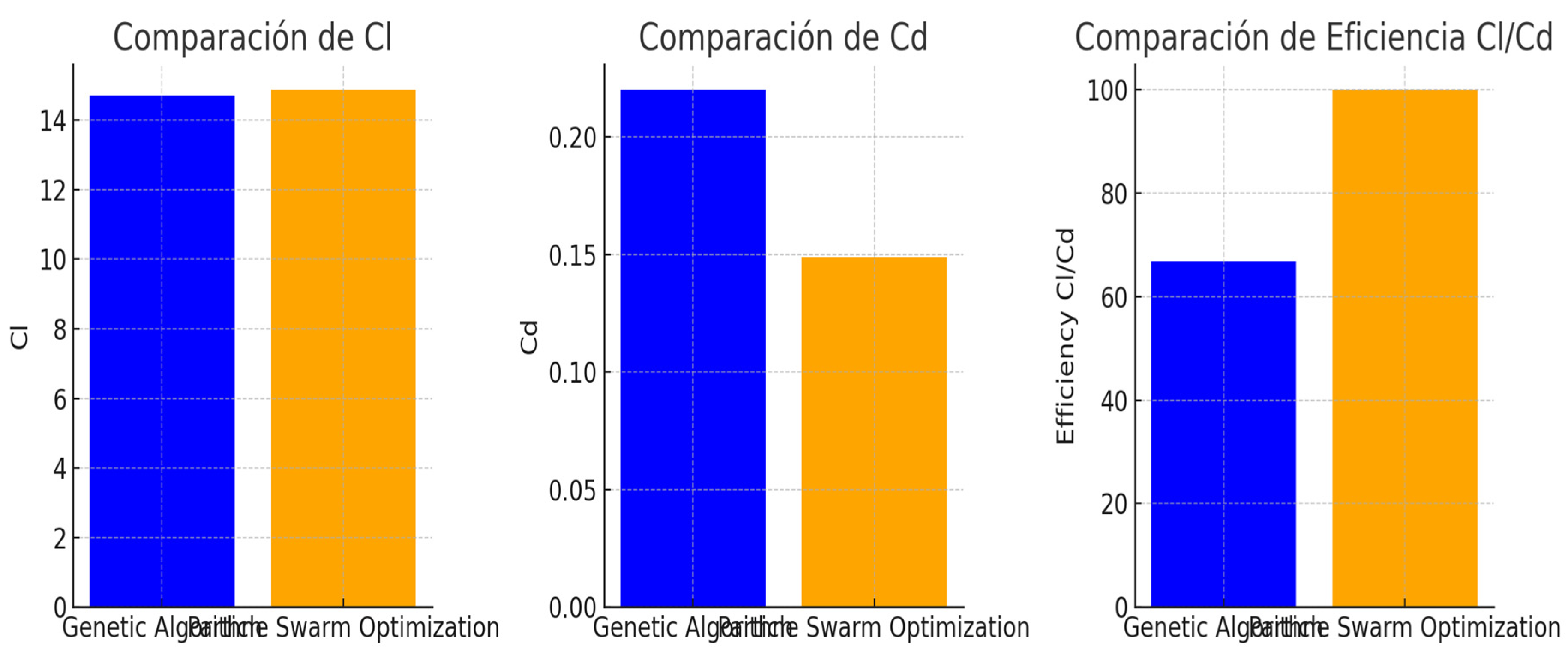
Figure 14.
Graphical displays of the results of the Genetic Algorithm (GA) and Particle Swarm Optimization (PSO) optimizations.
Figure 14.
Graphical displays of the results of the Genetic Algorithm (GA) and Particle Swarm Optimization (PSO) optimizations.
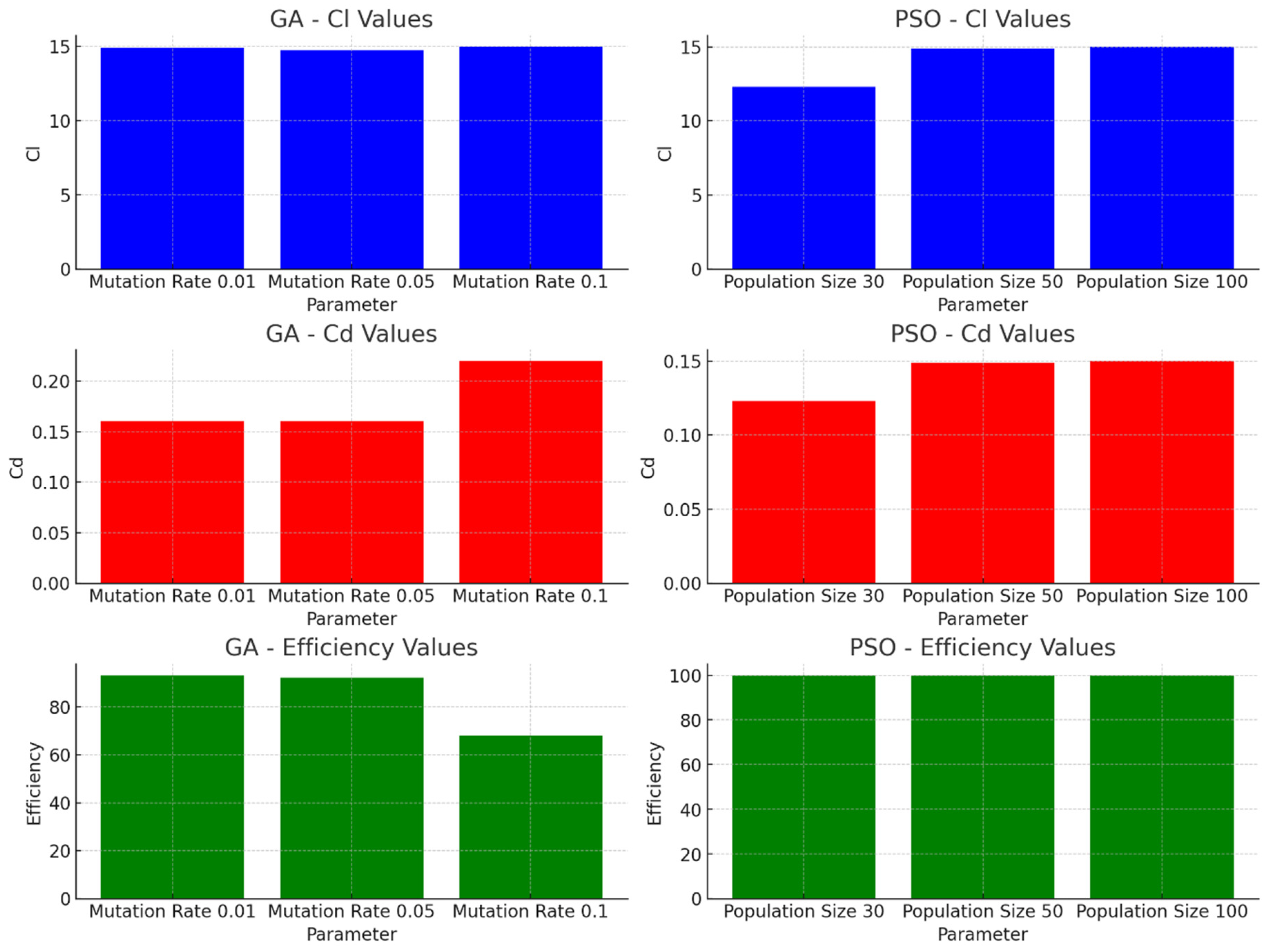
Figure 15.
Graphical displays of the results of the optimizations for the Genetic Algorithm (GA) and Particle Swarm Optimization (PSO), with different parameters.
Figure 15.
Graphical displays of the results of the optimizations for the Genetic Algorithm (GA) and Particle Swarm Optimization (PSO), with different parameters.
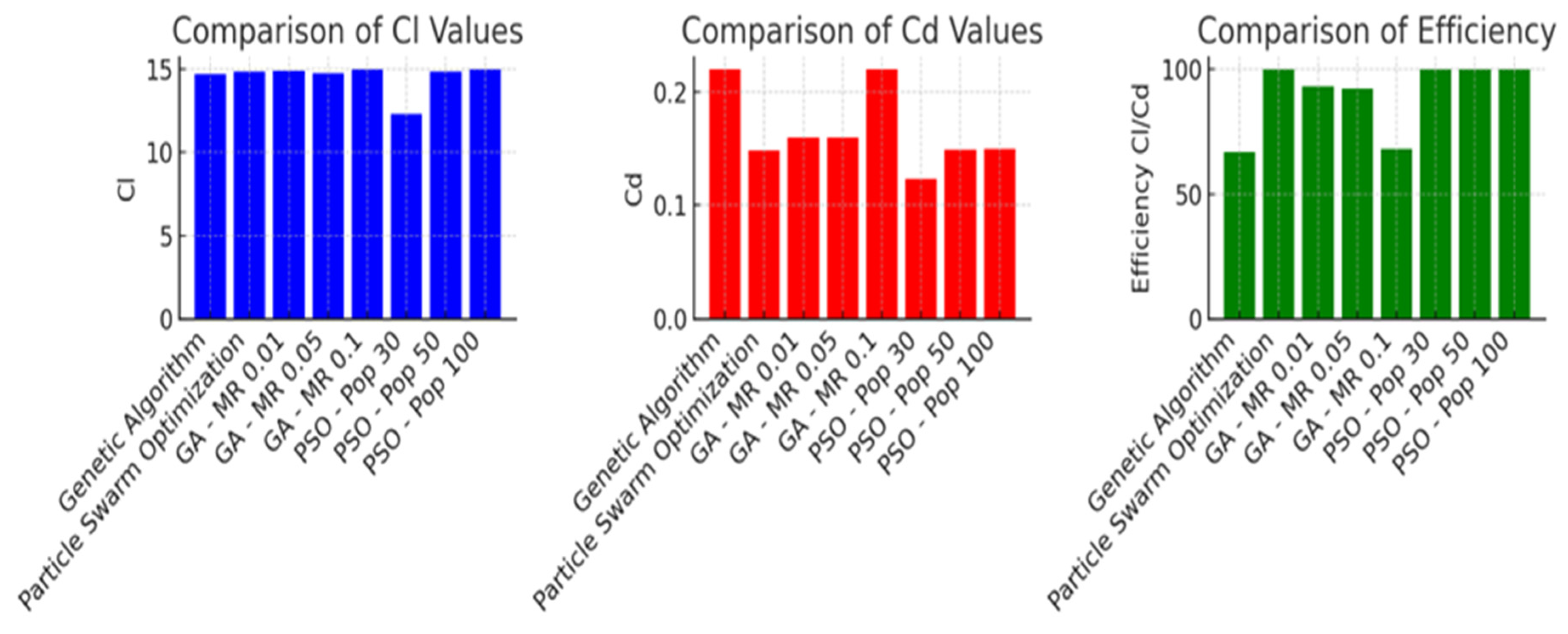
Figure 16.
Experimental COD abatement of the Alazine compared to that predicted by ANNi-GAs.
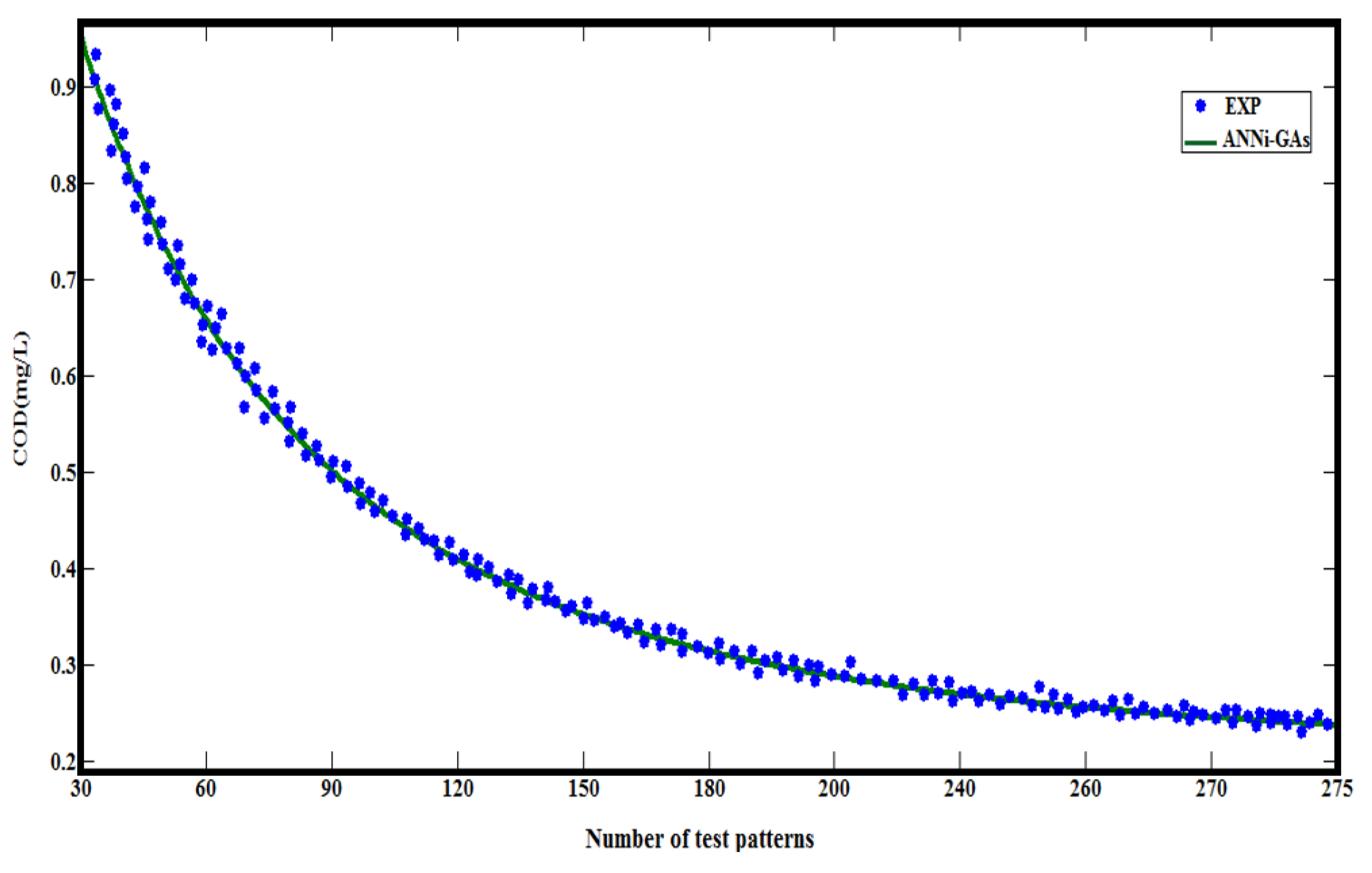
The model of ANNi-GAs has proven to be very effective in describing the reaction time for the chemical oxygen demand removal of herbicides during the degradation process, where the model was trained using experimental datasets and validated by the new datasets (fresh data). However, in practice, the calculations required for this system are complicated. Therefore, all the calculations were carried out on a Linux operating system, Intel D CPU 2.8 Ghz, and 4 GB of RAM. From these figures, the following results can be distinguished: The ANNi-GA model demonstrated the smallest error. In addition, we believe that our method could calculate the values of other input variables, but this was not done because it would significantly enlarge this paper. Throughout this investigation, the ANNi-GAs achieved better performance and agreed perfectly with the experimental data. Therefore, the coupling of an artificial neural network with genetic algorithms, as was done in our model ANNi-GAs, is a better choice for modeling the chemical oxygen demand due because the GAs search from a population (not a single point), including its parallel computing mechanism, and are also able to deal with the uncertainty of COD. These results provide vital evidence of the advantages of the proposed method. Therefore, it is believed that ANNi-GAs could be used to handle many other types of problems related to chemical oxygen demand removal during the aqueous treatment of herbicide degradation processes leading to the prediction.
6. Conclusions
The COD removal of herbicides during the degradation process was optimized using inverse artificial neural networks coupled with genetic algorithms to calculate an ideal input value from the COD, taking into account the above well-known input values, except the required input value as reaction time. Subsequently, the genetic algorithm was applied to the inverse problem to optimize the optimal operating conditions tested for a single parameter. Using this method, it was possible to find any unknown input variable online in the engineering water treatment of herbicide degradation. Indeed, it is very important to note that the elapsed time to calculate the optimum input parameter was less than one minute, thus it was feasible to obtain optimal parameters online and was sufficiently suitable for direct control of the degradation process in real time. Despite their success, ANNi-GAs are still in their infancy. This is a part of the future. In a way, it was amazing that we have done so much with so little, and we have barely begun. Consequently, if there are many input parameters to be found (solutions to multi-parameter problems), then genetic algorithms can solve the optimization problem. It is recommended that this approach be used to solve the optimization problem of high-dimensional functions. The development of this model could be carried out by implementing smart sensors for on-line estimated variables applied to the control and optimization of the engineering process under study, which should be observable, and we could expect an effect of the advanced oxidation process using sonophotocatalysis to operate more efficiently, indicating an appropriate reaction time to improve the COD value; however, these findings could be exploited in any situation where the estimation of inputs is needed. However, careful attention must be exercised when using this technique, related to its parameters, in which no physical meaning can be attached and operates with ad hoc mathematical tricks not directly dictated by basic physical principles.
References
- H. Köhler and R. Triebskorn, "Wildlife Ecotoxicology of Pesticides: Can We Track Effects to the Population Level and Beyond?".
- P. G. Dennis, T. Kukulies, C. Forstner, T. G. Orton and A. B. Pattison, "The effects of glyphosate, glufosinate, paraquat and paraquat-diquat on soil microbial activity and bacterial, archaeal and nematode diversity".
- M. Greaves, H. A. Davies, J. A. P. Marsh, G. I. Wingfield and S. J. L. Wright, "Herbicides and Soil Microorganisms".
- G. Rammohan and M. N. Nadagouda, "Green Photocatalysis for Degradation of Organic Contaminants: A Review".
- Y. Liu et al., "Photoelectrocatalytic degradation of tetracycline by highly effective TiO2 nanopore arrays electrode".
- Goli et al., "Applications of artificial neural networks for water quality prediction and modeling: A review," Sci. Total Environ., vol. 711, 2020, Art no. 137191. [CrossRef]
- N. A. Khan and S. M. Ali, "Artificial neural networks and genetic algorithm based model for prediction of dissolved oxygen in river," Environ. Sci. Pollut. Res., vol. 29, no. 43, pp. 65992–66009, 2022. [CrossRef]
- S. Heddam and S. Belkacem, "Inverse artificial neural network for the prediction of optimal operating conditions in a photovoltaic thermal collector," Mater. Today: Proc., 2021. [CrossRef]
- Khataee, A. R., Fathinia, M., Zarei, M., Izadkhah, B., Joo, S.W. 2014. Modeling and optimization of photocatalytic/photoassisted-electro-Fenton like degradation of phenol using a neural network coupled with genetic algorithm. Journal of Industrial and Engineering Chemistry. 20 (4). 1852-1860.
- Li, X., Maier, H. R., Zecchin, A. C. 2015. Improved PMI-based input variable selection approach for artificial neural network and other data driven environmental and water resource models. Environmental Modelling & Software. 65. 15-29.
- Hoffmann, M.R.; Martin, S.T.; Choi, W.; Bahnemannt, D.W. Environmental applications of semiconductor photocatalysis. Chem. Rev., 1995, 95(1), 6996.
- Herrmann, J.M. Heterogeneous photocatalysis: Fundamentals and applications to the removal of various types of aqueous pollutants. Catal. Today., 1999, 53(1), 115-129.
- Gaya, U.I.; Abdullah, A.H. Heterogeneous photocatalytic degradation of organic contaminants over titanium dioxide: A review of fundamentals, progress and problems. J. Photoch. Photobio. C., 2008, 9(1), 1-12.
- Wang, C., Quan, H., Xu, X., Optimal design of multiproduct batch chemical process using genetic algorithm. Industrial engineering and chemistry research,1996, 35, 10, 3560-6.
- Goldberg, D. E. (1989). Genetic algorithms in search optimization, and machine learning. Reading, MA: Addison Wesley.
- Baker, J.E. Adaptive selection methods for Genetic Algoriyhms. Pages 101-111 of proceedings of an international conference on Genetic Algorithms, Grefenstette, J.J. (ed), Lawrence Earlbaum. 1985.
- Frantz, D. R. Non-linearities in genetic adaptive search. Diss. Abstr. Int. B 1972, 33 (11), 5240.
- Jaimes-Ramírez R., Pineda-Arellano C.A., Varia J.C., Silva-Martínez S. Visible light-induced photocatalytic elimination of organic pollutants by TiO2: A Review. Current Organic Chemistry, 2015, 19, 540-555.
- Suslick, K.S., the chemical effects of ultrasound, Sci. Am., 1989, 260, 80-86.
- Hach Company, 1992. Water Analysis Handbook, Loveland, Colorado.
- David E. Goldberg. Genetic Algorithms in Search, Optimization, and Machine Learning.
- El Hamzaoui, Y., J.A. Hernandez, J. A., Silva-Martínez, S., Bassam, A., Alvarez, A., Lizama-Bahena, C., 2011. Optimal performance of COD removal during aqueous treatment of alazine and gesaprim commercial herbicides by direct and inverse neural network. Desalination. 37, 325-337.
- Hernández, J. A., Colorado, D., Cortés-Aburto, O., El Hamzaoui, Y., Velazquez, V., Alonso, B., 2013. Inverse neural network for optimal performance in polygeneration systems. Applied Thermal Engineering. 50. 1399–1406.
- Mas, D.M.L., & Ahlfeld, D.P. (2007). Comparing artificial neural networks and regression models for predicting faecal coliform concentrations. Hydrological Sciences.
- Journal, 52, 713-731.
- Crowther, J., Kay, D.,& Wyer, M.D. (2001). Relationships between microbial water quality and environmental conditions in coastal recreational waters: the fylde coast, UK. Water Research, 35, 4029-4038.
- Motamarri, S., & Boccelli, D.L. (2012). Development of a neural-based forecasting tool to classify recreational water quality using fecal indicator organisms. Water Research, 46, 4508-4520.
- A. J. F. Van Rooij, L. C. Jain, R. P. Johnson. Neural Network Training Using Genetic Algorithms. Series in Machine Perception and Artificial Intelligence. World Scientific Pub Co Inc (March 1997).
Figure 1.
General inverse artificial neural network model. where subscripts s and r are the number of neurons in the hidden layer and the number of neurons in the input layer, respectively; l is the number of neurons in the output layer; S is the number of neurons in the hidden layer; R is the number of inputs; Tansig is the hyperbolic tangent sigmoid transfer function; purelin is the linear transfer function; Wi, Wo and b1s; b2s are the input and output weights and biases, respectively.
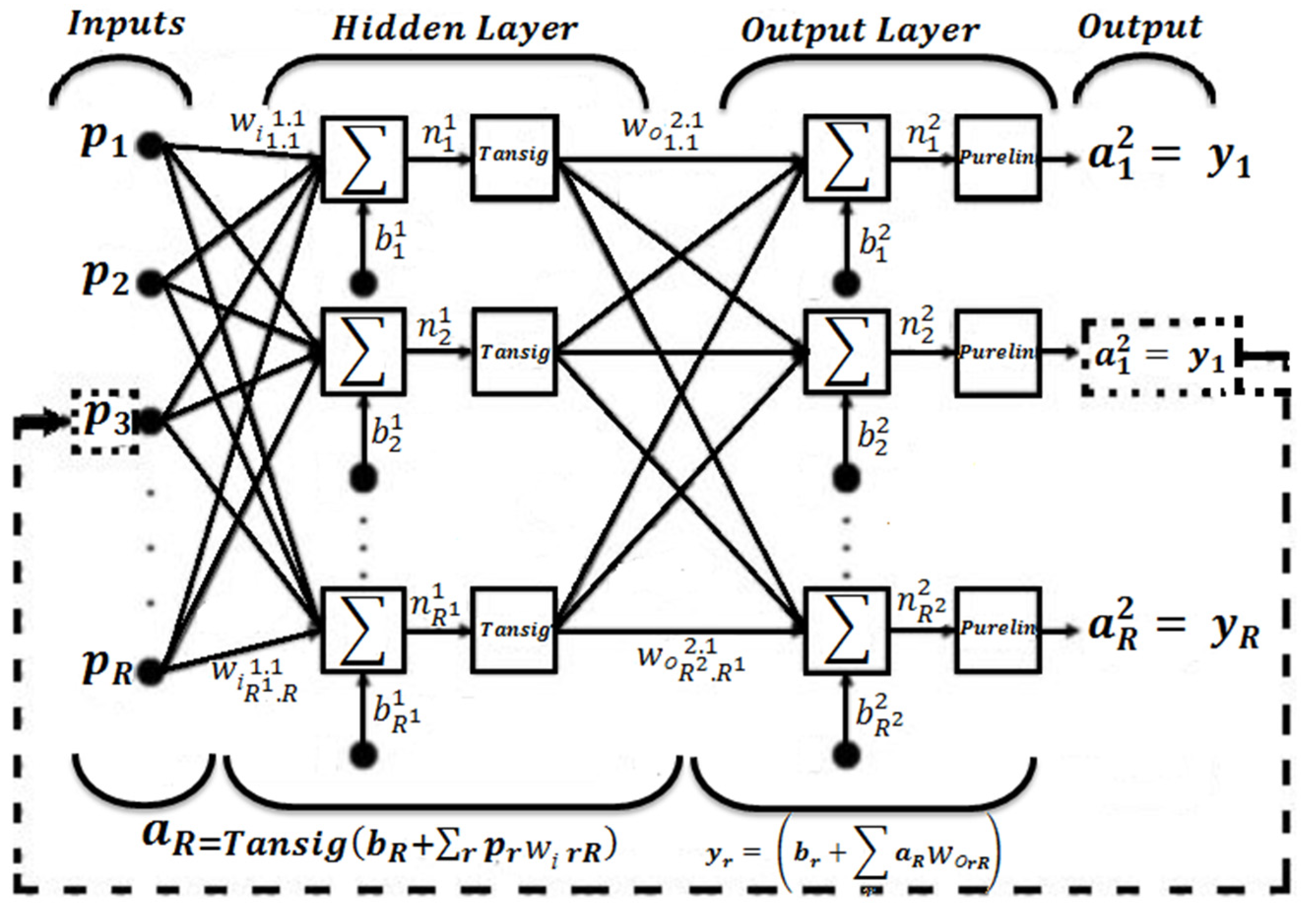
Figure 2.
Four-point crossover operators.
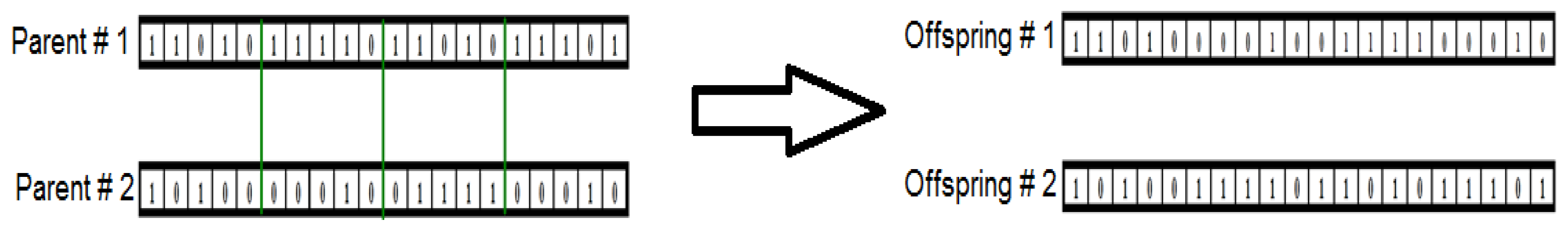
Figure 3.
Mutation of a chromosome at the 4th bit position.

Figure 4.
Evolution flow of genetic algorithms.
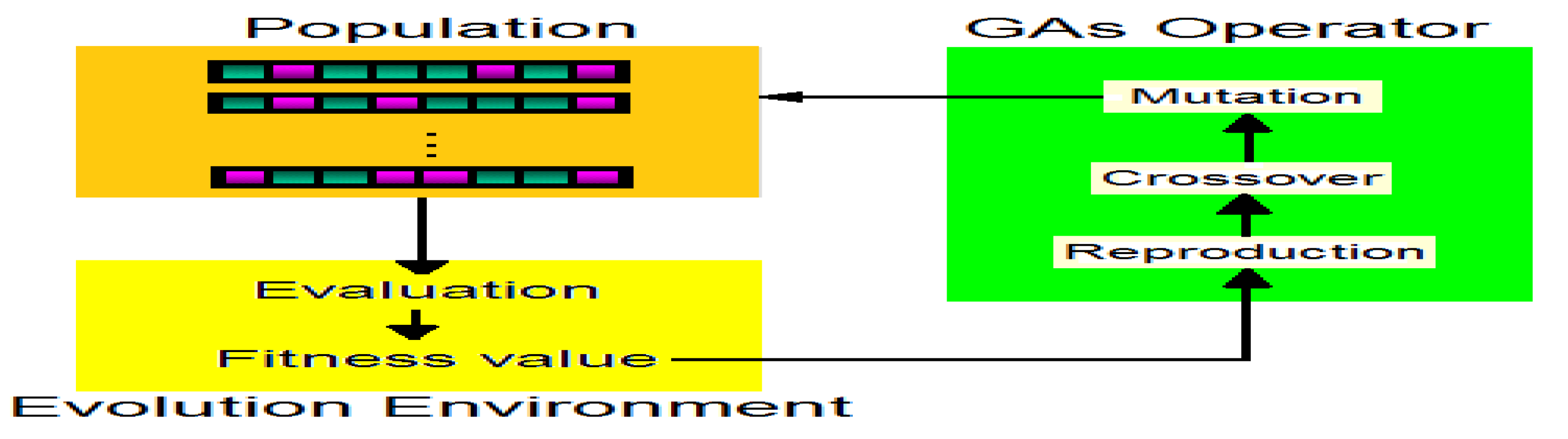
Figure 5.
Flowcharts of GAs.

Figure 6.
Numerical procedure used for the ANN learning process, and the iterative architecture used by the model to estimate the COD (S was the number of the neuron in the hidden layer).
Figure 6.
Numerical procedure used for the ANN learning process, and the iterative architecture used by the model to estimate the COD (S was the number of the neuron in the hidden layer).
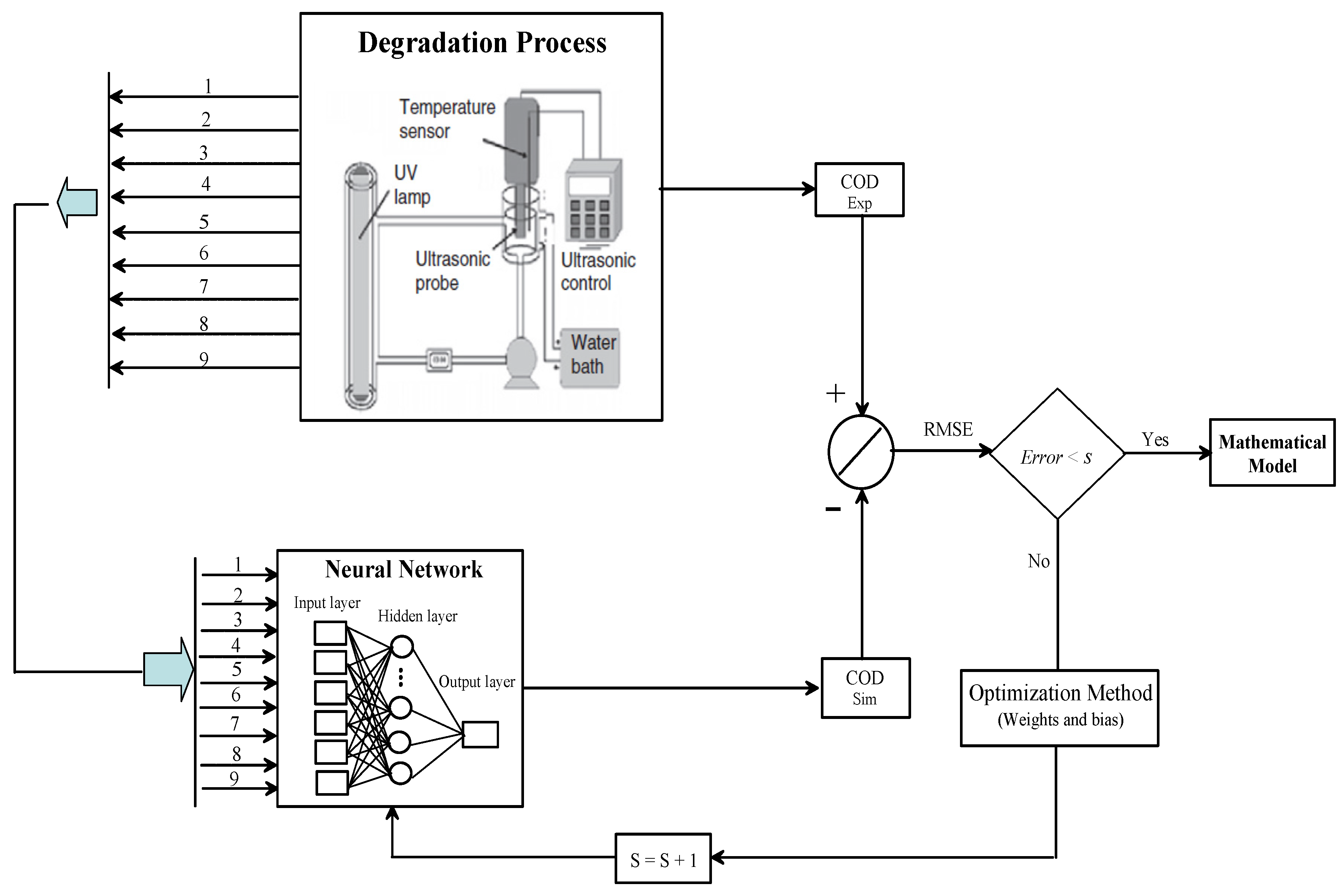
Figure 7.
Model for the prediction of COD values.
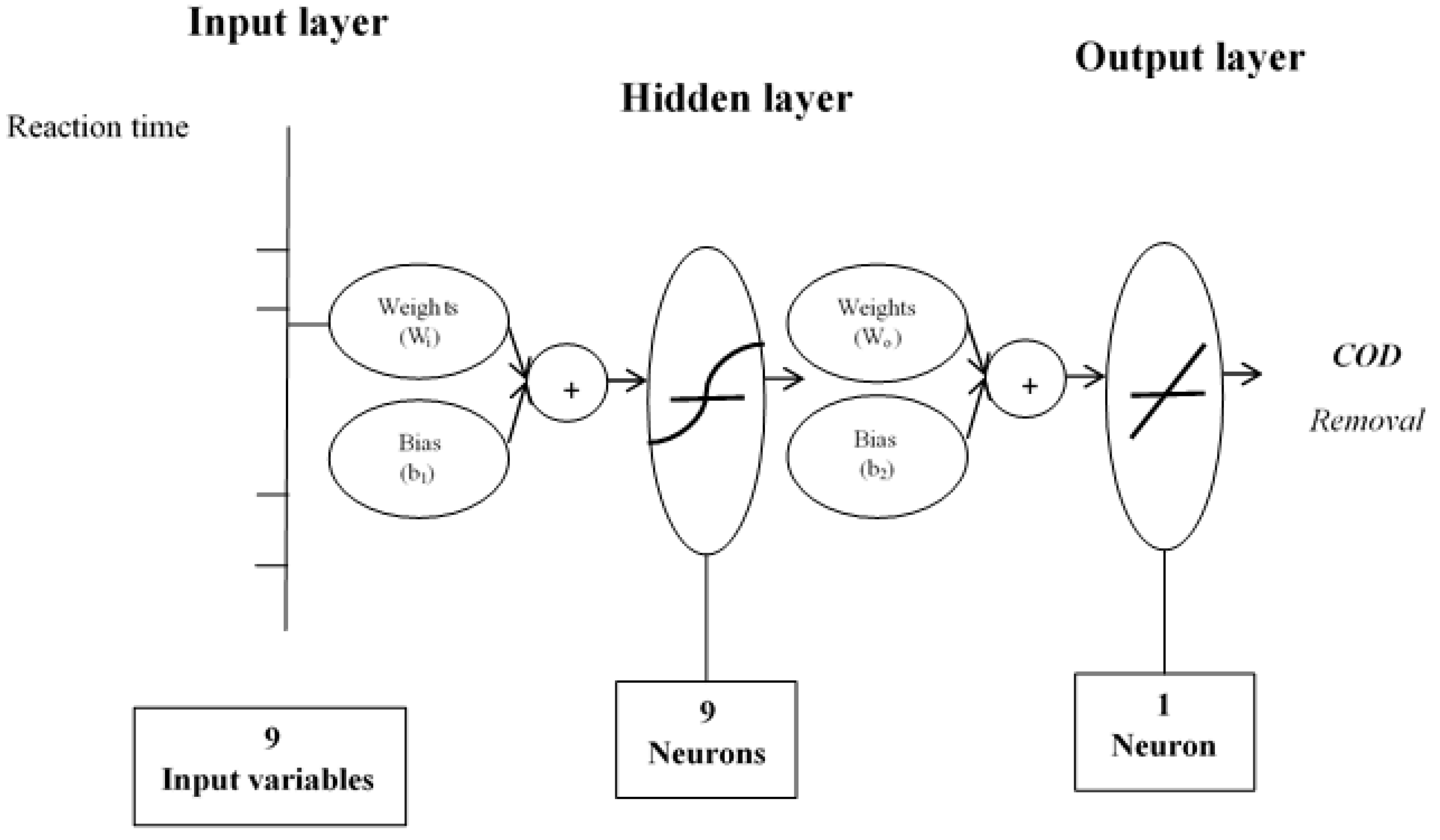
Figure 8.
Schematic methodology.
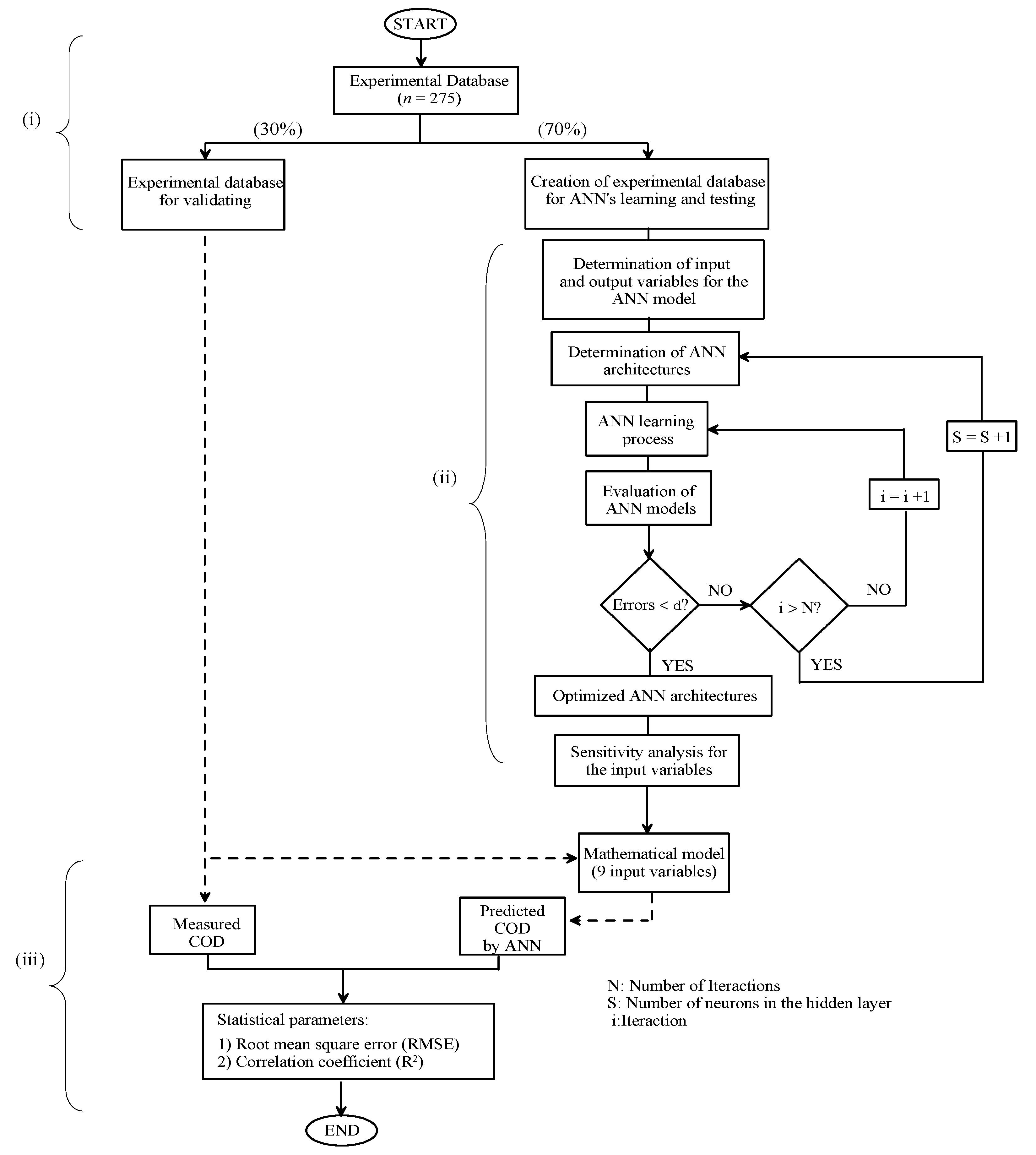
Figure 9.
Performance plots of ANN during training, validating and testing of the network.
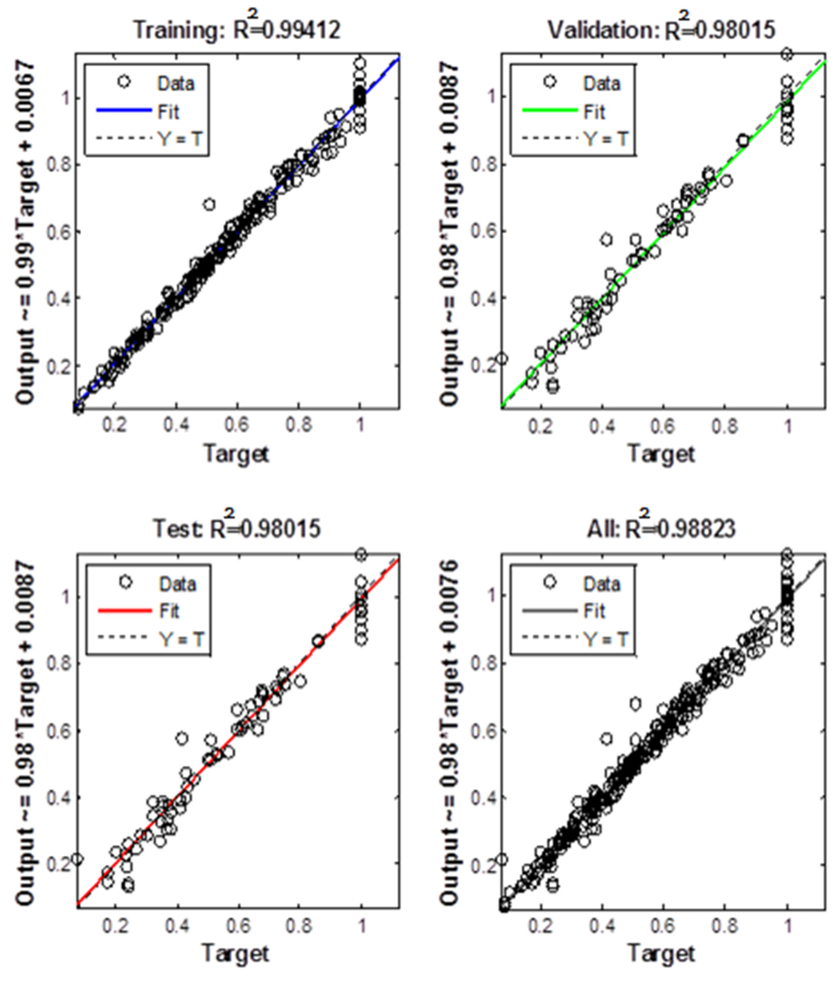
Figure 10.
The convergence for ANNi-GAs.
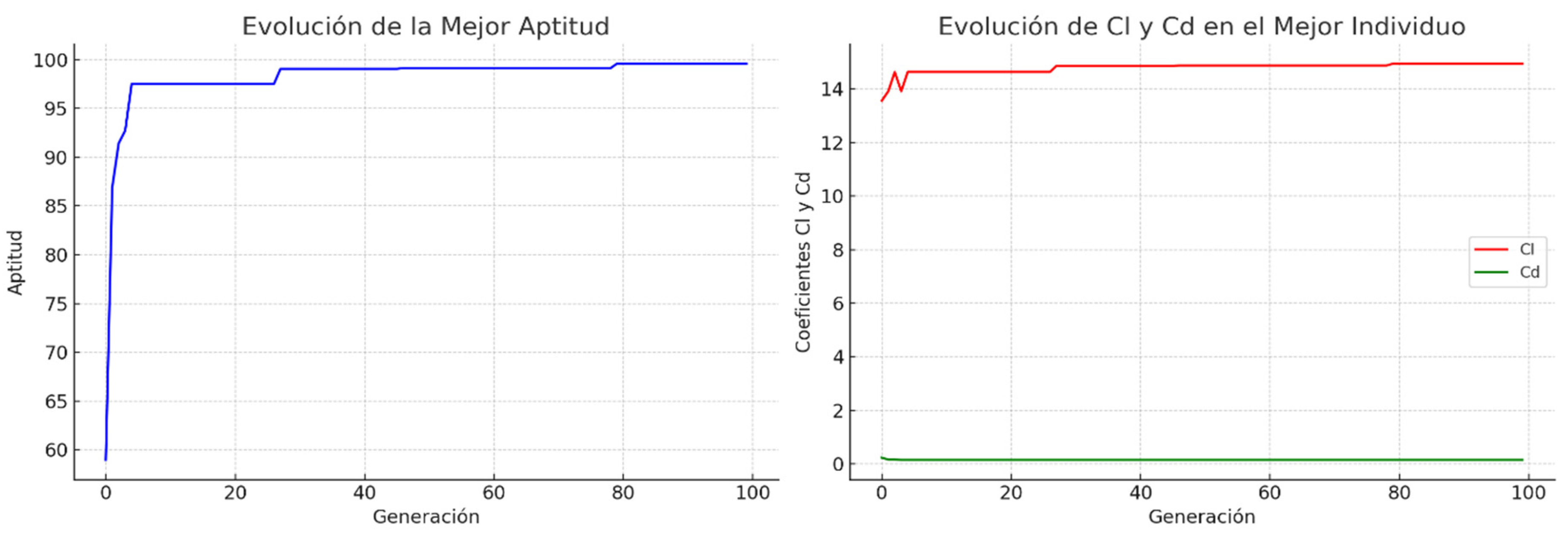
Figure 11.
Evolution of the best fitness including evolution of COD in the best individual with adjustments.
Figure 11.
Evolution of the best fitness including evolution of COD in the best individual with adjustments.
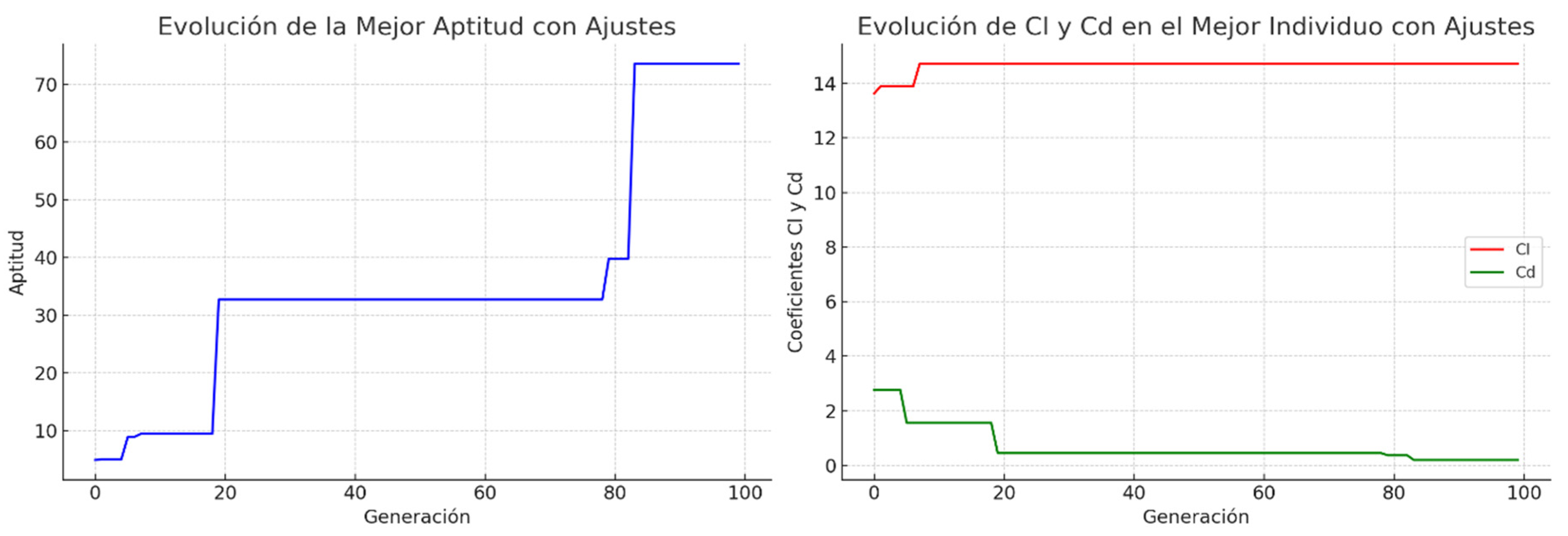
Figure 12.
Reaction time versus number of test patterns during herbicides degradation process.
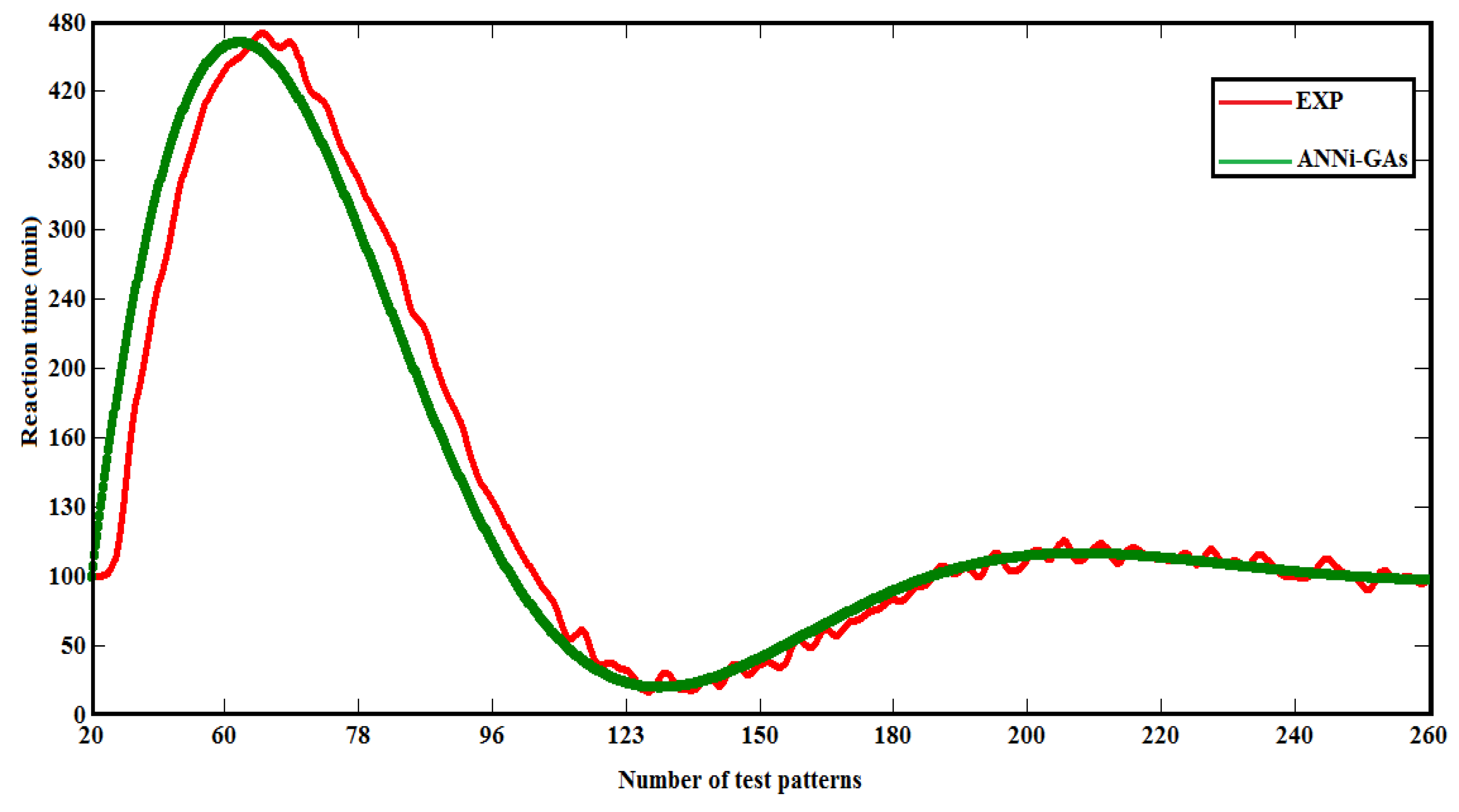
Table 1.
Experimental COD of alazine (comprised by alachlor and atrazine) and gesaprim (atrazine) including the reaction for the mineralization of the active compounds present in each herbicide.
Table 1.
Experimental COD of alazine (comprised by alachlor and atrazine) and gesaprim (atrazine) including the reaction for the mineralization of the active compounds present in each herbicide.
| Active components | Oxidation reaction (mineralization) | Concentration (mg/l) | COD (mg/l) |
|---|---|---|---|
| Alachlor | C14H20ClNO2 + 17O2 → 4CO2 + NH3 + HCl + H2O | 83.3 | 170.4 |
| Atrazine | C8H14ClN5 + 7.5O2 + H2O → CO2 + 5NH3 + HCl | 62.5 | 68.0 |
Table 2.
Characteristics of input and output parameters.
| Variable | Range | Unit |
|---|---|---|
| Input layer | ||
| Reaction time | 0 – 480 | min |
| pH | 1 – 5 | |
| Concentration of herbicides | 0.1540 – 0.3090 | mM |
| Contaminant | 0.1 – 0.9 | |
| US Ultrasound | 0 – 20 | kHz |
| UV Ultraviolet | 0 – 352 | nm |
| [TiO2]o | 0 – 300 | mg/l |
| [K2S2O8]o | 0 – 13 | mM |
| Solar radiation | 0 – 820 | W/m2 |
| Output layer | ||
| COD | 0.07 – 1 | mg/l |
Table 3.
Weights and biases for the ANN model.
| Number of neurons |
Weights | Bias | ||||||||||
|---|---|---|---|---|---|---|---|---|---|---|---|---|
| Hidden layer Wi (s, k) |
Output layer Wo (s, l) |
|||||||||||
| (s)* | (k=1) | (k=2) | (k=3) | (k=4) | (k=5) | (k=6) | (k=7) | (k=8) | (k=9) |
COD (l=1) |
b(1,s) | b(2,l) |
| 1 | -0.3166 | 0.2236 | 7.2842 | 2.0881 | 1.811 | 3.3471 | -1.0447 | 1.7596 | 2.0459 | 0.6031 | -5.25 | 12.9598 |
| 2 | -0.5515 | -0.956 | -3.8864 | 2.0139 | -2.867 | -1.294 | -0.45 | -6.4122 | 2.1782 | -5.9361 | 5.6355 | |
| 3 | 1.4092 | -8.029 | -12.034 | 15.7374 | -3.313 | -0.242 | -3.6828 | 11.6702 | -3.655 | 0.6256 | -11.9996 | |
| 4 | -0.7383 | -0.169 | -3.2518 | 1.2309 | -0.327 | -1.031 | -0.541 | -2.8458 | 1.668 | 7.0453 | 2.6748 | |
| 5 | 50.505 | -0.110 | 6.7242 | 1.7719 | -1.248 | -3.151 | 1.6575 | -1.4106 | -3.0969 | -6.087 | -2.4115 | |
| 6 | -1.3825 | -0.466 | -5.9643 | 5.8058 | 0.9334 | -2.855 | -1.6653 | -3.5912 | 2.8908 | -0.6846 | 1.2615 | |
| 7 | -29.020 | 0.7569 | 0.4108 | 0.2687 | -0.086 | -0.630 | 1.0245 | -0.7546 | -7.7876 | 5.127 | 1.4984 | |
| 8 | -3.7356 | 0.0012 | 0.9109 | -0.667 | -0.786 | -1.226 | 1.2131 | -1.3882 | -0.1462 | 1.7649 | -0.0617 | |
| 9 | -5.5039 | 1.1252 | 3.23 | -2.7131 | -0.735 | 0.2545 | 1.9287 | 3.0638 | -1.139 | -0.6662 | -0.6785 | |
| *s is the number of neurons in the hidden layer, k is the number of neurons in the input layer, l is the number of neurons in output layer (l=1). | ||||||||||||
Table 4.
Simulation results for the COD problem after 500 generations.
| Crossover type | Average of the runs2 | Geometric Mean of the runs3 | ||||
|---|---|---|---|---|---|---|
| 1-point | 0.515 | 0.583 | 0.379 | 0.401 | 6.81E-2 | 2.33E-2 |
| 2-point | 0.216 | 0.753 | 0.474 | 1.28E-2 | 5.02E-3 | 3.13E-3 |
| uniform | 0.113 | 0.183 | 0.203 | 9.52E-2 | 6.14E-3 | 3.17E-2 |
| NN-2-point | 0.553 | 0.277 | 0.927 | 3.35E-2 | 0.79E-3 | 7.01E-4 |
| NN-uniform | 0.376 | 0.305 | 0.229 | 3.47E-4 | 8.50E-5 | 9.12E-6 |
2The arithmetic mean is calculated as 3 The geometric mean is calculated as .
Disclaimer/Publisher’s Note: The statements, opinions and data contained in all publications are solely those of the individual author(s) and contributor(s) and not of MDPI and/or the editor(s). MDPI and/or the editor(s) disclaim responsibility for any injury to people or property resulting from any ideas, methods, instructions or products referred to in the content. |
© 2024 by the authors. Licensee MDPI, Basel, Switzerland. This article is an open access article distributed under the terms and conditions of the Creative Commons Attribution (CC BY) license (http://creativecommons.org/licenses/by/4.0/).
Copyright: This open access article is published under a Creative Commons CC BY 4.0 license, which permit the free download, distribution, and reuse, provided that the author and preprint are cited in any reuse.


