Preprint
Article

This version is not peer-reviewed.

Number-Operator-Based Inverse Engineering Technique for the Shortcut to Adiabaticity in Two Level Quantum Mechanical System

Submitted:

06 January 2025

Posted:

07 January 2025

You are already at the latest version

Abstract

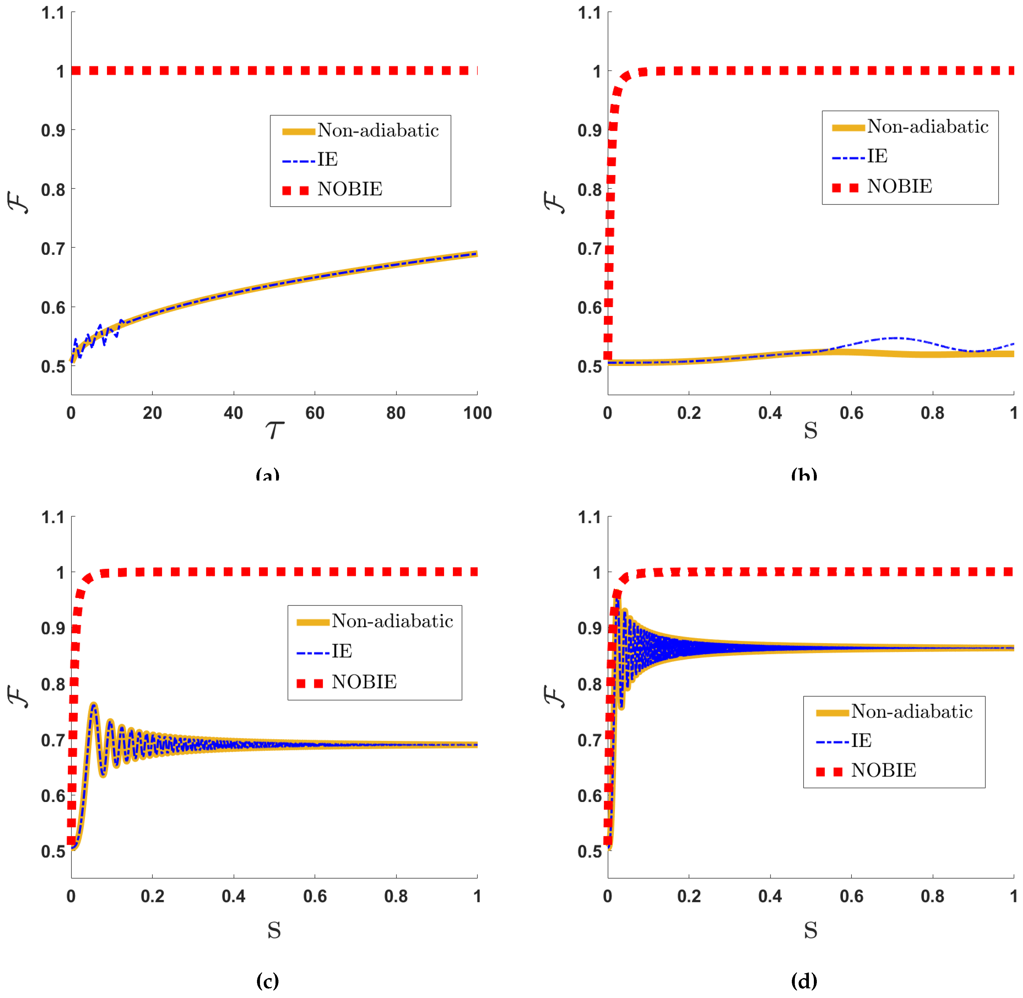
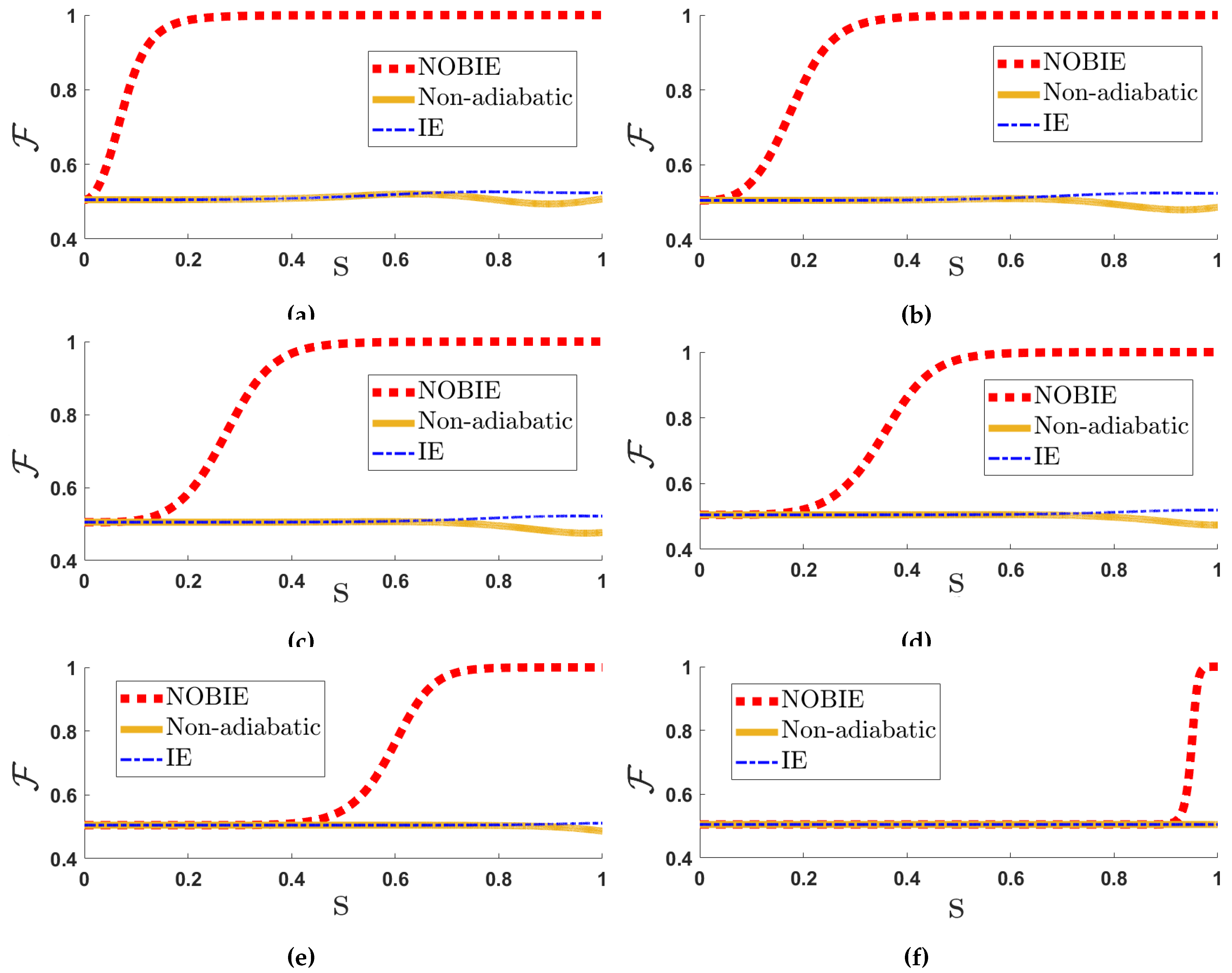
In general, the conventional Lewis-Riesenfeld invariant-based inverse engineering is a nonadiabatic process that results in the adiabatic final states to achieve the shortcut to adiabaticity, which does not provide complete suppression of non-adiabaticity throughout the evolution. We propose a new method to accomplish the shortcut to adiabaticity through an entirely adiabatic path. This new method is developed using the number operator as an invariant of the Hamiltonian. This paper discusses the mathematical framework of the new method in two-level quantum system and analyzes its performance compared to the conventional Lewis-Riesenfeld invariant-based inverse engineering method.

Keywords: 
;  ;  

1. Introduction

The adiabaticity in classical thermodynamics refers to the processes in thermally isolated systems [1]. However, the quantum mechanical definition of adiabaticity requires not only the isolation from the heat bath (environment) but needs to preserve the probability of occupation among the eigenstates [2,3]. Quantum adiabaticity is a relevant topic, considering its necessity in modern quantum technologies [4,5,6,7,8]. The quantum adiabatic theorem states that the process takes long time durations to achieve an entirely adiabatic evolution. This requirement of long time durations poses practical challenges to its testing and application. Quantum experiments and technologies deal with the preparation of quantum systems, quantum control, and quantum measurements; The needed time duration for quantum adiabaticity usually exceeds the coherence time of the prepared quantum systems [9]. Further, the technologies like quantum heat engines can produce only a negligible power output due to the long time duration of cycles [8]. Thus, the reduction of the time duration to achieve an entirely adiabatic process is in the research front over the last decade [10,11,12,13,14,15,16,17,18,19]. The attempts for the same succeeded in bringing several methods collectively called the shortcut to adiabaticity (STA) [2,3].
STA methods provide protocols to drive the quantum systems to an adiabatic final state corresponding to the system’s initial state. These protocols are theoretically optimized to give accurate results in short time durations. Several methods to achieve STA differ in the approach to developing protocols. Let us consider the theoretical approach of the counter-diabatic (CD) method [10,11,12] and invariant-based inverse engineering (IE) [14,15,16,17,18,19]. The CD method restructures the Hamiltonian to get the approximate adiabatic solution as the general solution of the time-dependent Schrodinger equation [10]. The above approach cancels the non-adiabatic excitations throughout the evolution, and the process follows an entirely adiabatic path. The IE method uses the Lewis-Riesenfeld (LR) invariants of the Hamiltonian and some boundary conditions to obtain the STA protocol. This method gives more freedom to arbitrarily fix the protocols and explore different paths to reach the final adiabatic state. Equivalent to say that the method produces a class of inverse engineered Hamiltonians to drive the system to a final adiabatic state. The CD method lacks this arbitrary set of protocols, and the IE method will not evolve through the entirely adiabatic path in general [3]. We use the number operator as an invariant of the Hamiltonian to develop protocols that drive the quantum system in an entirely adiabatic path, and prove that the Number-operator-based inverse engineering (NOBIE) method can generate a class of Hamiltonians to achieve STA. Also, we illustrate the new method for two-level systems.
Two-level systems are the most simple but essential systems for understanding quantum-level dynamics [20]. The two-level systems were vital in developing quantum theory from the early days. The quantum theory advanced from a subject explaining the quantumness in nature to engineering quantum systems with desired quantum effects, and the two-level systems became an inalienable part of modern-day quantum technologies. The usage of two-level systems ranges from the Stern-Gerlach experiment to qubits for quantum computation and information. Any combination of three Pauli spin matrices can represent a Hamiltonian to drive two-level systems [21]. Among numerous such possibilities, the Landau-Zener (LZ) Hamiltonian might be the one that is widely studied [22,23,24,25,26]. Existing STA methods were applied and tested for LZ dynamics [3], and this paper illustrates the NOBIE method for the LZ Hamiltonian. We verify the credibility of the NOBIE method using a numerical simulation of the fidelity of the shortcut process. Also, this paper compares the performance of the conventional IE method and the NOBIE method from the fidelity plots.

2. IE and NOBIE Methods for Two-Level Systems

We begin this section by considering the LZ Hamiltonian [8],
H = z x x z ,
to drive the two level quantum system. The LZ dynamics depend on the linearly time-dependent variation of z with a constant x. In other words, the LZ Hamiltonian is a combination of the Pauli-Z operator with a linearly time-dependent function,
z = z ( 0 ) + z ( τ ) z ( 0 ) t τ
and a Pauli-X operator with a constant, x. Here, τ is the total time duration of the driving process, and t represents time. The initial state of the two level system, | ϕ ( 0 ) , changes during the driving with LZ Hamiltonian and attains a state, | ψ ( τ ) on completion of the process. The variation of a quantum system’s state during a time-dependent driving can be understood from the parameter called fidelity [8,27],
F = | ψ ( τ ) | ϕ ( τ ) | 2
where | ϕ ( τ ) is the adiabatic final state. If the state obtained after the driving is the same as the adiabatic final state, then the fidelity will be unity ( F = 1 ). Otherwise, the fidelity takes a value between zero and one. Thus, the fidelity will be unity for a successfully completed adiabatic process/shortcut process, and any deviation from the final adiabatic state results in 0 F < 1 . We can generate F by numerically simulating the time-ordered exponential of the Hamiltonian. The precise method of numerical simulation of time-ordered exponential is provided in Appendix A.
Figure 1a shows the fidelity for the non-adiabatic driving of different time durations (in arbitrary unit) using the Hamiltonian in equation (1) (solid yellow line). We have assumed z ( 0 ) = 0 , z ( τ ) = 10 , and the constant x = 0 . 1 . The fidelity of the non-adiabatic drive increases with the increase in the time duration of the process. However, the fidelity is very low for short time durations. The evolution paths of LZ driving for different time durations are depicted in figures 1b-1d (solid yellow line). It moves towards the entirely adiabatic path for an increased time duration of the process. However, the fidelity fluctuates throughout the path, showing the drive’s instability. The non-adiabaticity and instability of the LZ dynamics are evident from the above mentioned figures. Further, developing a conventional IE method and NOBIE method will enable us to compare the fidelities. Let us revisit the conventional inverse engineering method for two-level systems.

2.1. IE Method for Two-Level Systems

The IE method was developed based on two fundamental concepts in quantum mechanics. The first concept is that an operator/observable which is invariant in the Hilbert space of the Hamiltonian satisfies the relation [14],
I t = i I , H
where the invariant, I and Hamiltonian, H are the time-dependent operators. The time dependence of H is determined by its control parameters (z for LZ Hamiltonian), while I contains arbitrarily chosen time-dependent functions. The above equation can inverse engineer the control parameters of H from the arbitrary parameters of I . Secondly, the commuting operators share a common set of eigenstates, which helps to set the boundary conditions guiding the protocol to the final adiabatic state [21]. The boundary conditions are obtained using the relations [8],
I ( 0 ) , H ( 0 ) = 0
and
I ( τ ) , H ( τ ) = 0
Let us understand the step-by-step mathematical formulation of the IE method for a two level system driven by the LZ Hamiltonian in equation (1). Assume the invariant of the form,
I = c a i b a + i b c ,
where a , b , and c are arbitrary time-dependent parameters. These parameters can be designed so that the invariant will satisfy the condition in equation (4). For the above purpose, we have to substitute the assumed form of invariant and the LZ Hamiltonian to the invariance condition (4). Then, we obtain the following conditions relating to the arbitrary parameters of I and the control parameters of H ,
a ˙ = 2 b z ,
b ˙ = 2 a z 2 c x ,
c ˙ = 2 b x ,
where the dot accent represents the time derivative. We can rewrite all the arbitrary parameters of the invariant in terms of c and its time derivatives. From equation (9), we can write b = c ˙ 2 x , and from equation (8), we get a = c ¨ 4 x z + c x z . Thus, the explicit form of the invariant becomes,
I = c c ¨ 4 x z + c x z i c ˙ 2 x c ¨ 4 x z + c x z + i c ˙ 2 x c .
Using the property that the eigenvalue of an invariant is a constant [14], we can write,
A 2 = c ¨ 4 x z + c x z 2 + c ˙ 2 x 2 + c 2 ,
where A is the constant eigen value of the invariant. On rearranging the above equation, we get an expression for z in terms of other parameters. The obtained explicit form is
z = c ¨ 4 x + c x A 2 c ˙ 2 4 x 2 c 2 1 2 .
The above two equations (11) and (12) help inverse engineer the LZ Hamiltonian. In other words, the LZ Hamiltonian with z defined in equation (12) satisfies the invariance condition with the invariant in equation (10). Further, we need to apply the boundary conditions to achieve STA. For that we substitute the LZ Hamiltonian in equation (1) and invariant in equation (10) to equations (5) and (6) and obtain
c ˙ ( 0 ) = c ˙ ( τ ) = c ¨ ( 0 ) = c ¨ ( τ ) = 0 .
Thus, an arbitrary function c which satisfies the above boundary conditions, can inverse engineer the LZ Hamiltonian using equation (12) to achieve STA. We choose a particular function [8],
c = z ( 0 ) + 6 z ( τ ) z ( 0 ) t τ 5 + 10 z ( τ ) z ( 0 ) t τ 3 15 z ( τ ) z ( 0 ) t τ 4 ,
which satisfies the required boundary conditions to inverse engineer the LZ Hamiltonian. The numerical simulation of time-ordered evolution of inverse engineered LZ Hamiltonian provides the fidelity as given in Figure 1a (dot-dashed blue line). Compared with the fidelity of the non-adiabatic drive (solid yellow line), the STA based on the conventional IE method is not enough to improve significantly. The fidelity of the IE method shows some fluctuations for short time durations, while it merges with the fidelity of the non-adiabatic drive for long time durations. The evolution path for the IE method (dot-dashed line in figures 1b-1d) also shows the exact characteristics of the non-adiabatic drive without any improvement. Although, the original formalism of the IE method claims to achieve adiabatic final state in arbitrarily short time durations, the cost ( C ) of implementation also plays a vital role in its successful completion. The cost of implementation for successful completion of STA methods increases as the time duration of the process decreases [27,28,29]. In our previous paper [8], we have discussed the implementation of the invariant-based STA method in qubits for varying cost. And we found the cost required to achieve the adiabatic final state increases for decreasing time duration of the STA process. Also, for a specified short time duration, the invariant-based STA method (Ref. [8]) unsuccessful to achieve the adiabatic final state for cost values below the required cost of successful implementation. Similarly, in this work, Figure 1a shows that the IE method unsuccessful to achieve final adiabatic state in short time durations, which implies the insufficient cost of implementation. Choosing a different arbitrary function c might change the cost of implementation and improve the fidelity of the drive for given time durations. However, it is not ideal to arbitrarily guess the c function until we improve fidelity. In the following subsection, we develop the NOBIE method to achieve STA through an entirely adiabatic path and compare its fidelity with non-adiabatic and IE fidelities. The comparison is performed for time durations for which the conventional IE method unsuccessful to achieve STA. Also, a comparison of the cost of the IE and NOBIE methods is provided towards the end of this section.

2.2. NOBIE Method for Two-Level Systems

As we mentioned in the introduction, quantum adiabaticity requires isolation from the environment and preservation of probability among the eigenstates. The first mentioned can be achieved by perfecting the experimental setup, while the latter depends on the driving protocol and time duration of driving. We aim to preserve the probability among the eigenstates, although in a short time. Such a short process through an entirely adiabatic path can be developed based on an invariant that commutes with the system Hamiltonian for the whole driving duration. We define a number operator for the system Hamiltonian and use it as an invariant for the above purpose. Let us see why the invariance of the number operator leads to driving through an entirely adiabatic path.
Figure 1. (a) Fidelity of the non-adiabatic driving (Solid yellow line), IE method (dot-dashed blue line), and NOBIE method (dotted red line) are plotted against the total time duration of the process, τ . The evolution path of the non-adiabatic driving (Solid yellow line), IE method (dot-dashed blue line), and NOBIE method (dotted red line) are plotted against ratio s = t / τ for different τ values, (b) τ = 1 (c) τ = 100 , and (d) τ = 500 . The parameters z ( 0 ) = 0 , z ( τ ) = 10 , and x = 0 . 1 are used for the calculation. Time is considered in arbitrary units for all the plots.
Preprints 145307 g001
Consider the spectral decomposition of the system Hamiltonian [21],
H = n λ n | n n | ,
where λ n is the energy eigenvalues, | n is the instantaneous eigenstates, and n is the quantum number. In general, λ n is a time-dependent function that also depends on the corresponding quantum number. If it is possible to write the energy eigenvalues in a separable form as a product, λ n = g ( n ) f ( t ) ( g ( n ) is a function of n alone and f ( t ) is a function of t alone), then, we can define a number operator,
N = H f ( t ) = n g ( n ) | n n | .
As N is just a scaling of system Hamiltonian by a function of time alone, N will always commute with H . It is essential to prove that the invariance of the number operator leads to the preservation of the probability among the eigenstates. Let us find the expectation value of the number operator for that purpose,
Figure 2. The cost ratio of NOBIE and IE methods for time durations of the process ( τ ) ranges from 1 to 10. The black dotted line corresponds to the cost ratio with k = 1 and the blue solid line corresponds to the cost ratio with k = 2 . All the other required parameters are same as in Figure 1
Preprints 145307 g002
N = ψ | N | ψ ,
where | ψ is the general solution of the time-dependent Schrodinger equation. We can decompose | ψ on to the instantaneous eigenstates | n using time-dependent coefficients, C n as [21]
| ψ = n C n | n .
Substituting the above expression for | ψ to equation (16), we obtain,
N = n C n 2 n | N | n = n C n 2 g ( n ) ,
where C n 2 is the probability of occupation among the instantaneous eigenstates, which is a function of time. The above equation clearly says that the constant probability among the instantaneous eigenstates corresponds to the constant expectation value of the number operator. The converse of the above statement is also true: if g ( n ) is distinct for all the eigenstates, then a constant expectation value of the number operator results in a constant probability of occupation among the eigenstates. Thus, a Hamiltonian that obeys the invariance condition with the number operator is needed to drive the system through an entirely adiabatic path. We assume that a NOBIE Hamiltonian H N satisfies the invariance condition:
N t = i N , H N .
In the case of LZ Hamiltonian, the energy eigenvalues are given by λ n = ± z 2 + x 2 , which gives
g ( n ) = ± 1
and
f ( t ) = z 2 + x 2
Then the number operator corresponding to the LZ Hamiltonian becomes
N = H f ( t ) = 1 z 2 + x 2 z x x z
Considering the structure of N , we should choose H N = y σ y , where y is an arbitrary function of time. Then, the commutation of H N with the number operator results in an operator of σ x and σ z combination (as same as the combination of the left-hand side of the above equation). Substituting the explicit form of N and H N to the invariance condition (equation (19)) will result
z ˙ f ( t ) z f ˙ ( t ) f 2 ( t ) x f ˙ ( t ) f 2 ( t ) x f ˙ ( t ) f 2 ( t ) z ˙ f ( t ) + z f ˙ ( t ) f 2 ( t ) = 2 y x f ( t ) 2 y z f ( t ) 2 y z f ( t ) 2 y x f ( t ) ,
from which we can deduce two relations,
z ˙ f ( t ) z f ˙ ( t ) f 2 ( t ) = 2 y x f ( t )
and
x f ˙ ( t ) f 2 ( t ) = 2 y z f ( t )
Adding equation (24) multiplied by x and equation (25) multiplied by z gives
x z ˙ f ( t ) = 2 y x 2 + y 2 f ( t ) = 2 y f ( t )
The above equation results in the arbitrary function of inverse engineered Hamiltonian,
y = x z ˙ 2 f 2 ( t )
and explicitly, we can write,
H N = 0 i x z ˙ 2 f 2 ( t ) i x z ˙ 2 f 2 ( t ) 0 .
We have simulated the time-ordered evolution of the two level system using the above NOBIE Hamiltonian. The obtained fidelity for various time durations is plotted in Figure 1a (red dotted line). The performance of the newly developed method is as expected and always gives near to unit fidelity irrespective of the time duration of the process. The path of evolution using H N for various time durations are given in figures 1b-1d (red dotted line). The path deviates from the entirely adiabatic path ( F = 1 ) at the initial moments of the drive. However, the NOBIE methods attain complete adiabaticity in the early instants of drive, while the non-adiabatic and conventional IE methods usually unsuccessful to attain the same. The stability of the NOBIE method to maintain the unit fidelity is commendable compared with the fluctuating non-adiabatic and IE methods. The trend of evolution path by NOBIE method is similar irrespective of the total time duration of the process, which is highly desirable.
Figure 3. The evolution path of the non-adiabatic driving (Solid yellow line), IE method (dot-dashed blue line), and NOBIE method (dotted red line) are plotted against ratio s = t / τ ( τ = 1 ) for different control functions z = z ( 0 ) + z ( τ ) z ( 0 ) t m τ , where m takes values, (a) m = 2 , (b) m = 3 , (c) m = 4 , (d) m = 5 , (e) m = 10 , and (f) m = 100 . The parameters z ( 0 ) = 0 , z ( τ ) = 10 , and x = 0 . 1 are used for the calculation. Time is considered in arbitrary units for all the plots.
Preprints 145307 g003
As it is already mentioned, the unsuccessful of the IE method in achieving adiabatic final state is a consequence of inefficient cost of implementation. Then, it becomes necessary to compare the cost for both IE and NOBIE methods to understand the merits or demerits of the new method. The cost as a measure of resources involved in the implementation of a shortcut, it does not have a unique definition. There are multiple definitions for the cost and this paper use a recent definition [3,27,30],
C 0 τ | | H | | k d t , k = 1 , 2 , 3 . . .
where | | H | | = t r a c e H H is the Frobenius norm and H is the Hamiltonian driving the system i.e., substituting the inverse-engineered Hamiltonian gives the cost for IE method ( C I ) and NOBIE Hamiltonian gives the cost for NOBIE method ( C N ). The cost depends on the quantum system and the fields used to implement the Hamiltonian, since the value of k is associated with power required to generate the control fields [3]. For example, the value of k = 1 for a neutral atom in a time-dependent electric field, and k = 2 for a single spin system in a time-dependent magnetic field [30].
The propotionality relation of cost for the IE and NOBIE methods can be obtained by substituting the respective driving Hamiltonians in equation (29). Further, the ratio of the cost gives,
C N C I = 0 τ x 2 + z 2 k d t 0 τ y k d t ,
where z is given by equation (12). In Figure 2, we have plotted the above cost ratio with k = 1 , 2 for time durations of the process ranging from 1 t o 10 . The obtained value of cost ratio is less than one implying that the cost for NOBIE method is always less than that of the IE method. The indicated costs for the process in unit time duration ( τ = 1 ) reveals that the magnitude of NOBIE cost is very small compared with that of IE method ( C N = 0 . 0857 C I for k = 1 and C N = 0 . 285 C I for k = 2 ). Also, the cost ratio decreases with increase in the time duration of the process. This analysis clearly shows the advantage of the NOBIE method that it succeeded to achieve the final adiabatic state for time durations for which IE method is unsuccessful and with lesser cost than the cost of IE method.
All the fidelity calculations in Figure 1 and Figure 2 are based on the linear variation of the control parameter z as given in equation (2). It is possible to analyze the performance of STA methods for different control parameters of the LZ Hamiltonian. A class of control parameters, z = z ( 0 ) + z ( τ ) z ( 0 ) t m τ can be defined for the varying rate of change of the control parameter with values of m. In Figure 3, we have compared the evolution path of the non-adiabatic, IE, and NOBIE methods for m = 2 , 3 , 4 , 5 , 10 , and 100. The total time duration for all the plots is fixed as unity, τ = 1 . The IE method still unsuccessful to achieve the final adiabatic state for all the values of m. The increase in the value of m increases the rate of change of the control parameter and energy ( λ n ). The high rate of change of energy affects the entirety of the adiabatic path of the NOBIE method, and the deviation of the NOBIE method’s fidelity curve from unit fidelity increases with increasing values of m. However, the NOBIE method achieves unit fidelity (adiabatic state) towards the end of the drive for a dramatically high energy change rate with m = 100 , assuring the final adiabatic state.

3. Discussion

A shortcut to adiabaticity through an entirely adiabatic path is the motivating factor for the new method, NOBIE. As the driving protocols based on the invariance of the number operator are theoretically optimized to get an entirely adiabatic path, the stability of the protocol is presumably higher than that of the conventional IE method. From all the comparisons (Figure 1 and Figure 3), it is evident that the stability of the method to achieve the final adiabatic state is far better than the conventional IE method in short time durations. To see the cancellation of the the non-adiabatic transitions throughout the evolution of NOBIE dynamics, find the expression for the non-diagonal elements of H N in the instantaneous eigen basis of H using the equation (19),
n | H N | m = i n | N t | m g ( m ) g ( n ) .
Also, from the definition of number operator, we can get,
n | H t | m = f ( t ) n | N t | m .
Combining above two equations results
n | H N | m = i n | H t | m λ m λ n ,
which is equivalent to the off-diagonal elements of the counter-diabatic Hamiltonian in energy eigen basis [10]. Although the off-diagonal elements of NOBIE and counter-diabatic methods are equivalent, the method of deriving Hamiltonian for shortcut to adiabaticity is completely different. This equivalence justifies the entirely adiabatic path of the NOBIE method. Also, the fidelity curves obtained for NOBIE method will be same as that of CD method for two-level system governed by LZ Hamiltonian (see the Appendix B).
The driving Hamiltonian for STA resulting from the NOBIE method is not unique, but it provides a class of NOBIE Hamiltonians to drive the system. It is possible only due to the mathematical formalism of the entirely adiabatic path. In the NOBIE the number operator always commutes with system Hamiltonian (see equation (15)),
N , H = 0 .
This relation is useful to see that the addition or subtraction of arbitrary times the system Hamiltonian from the NOBIE Hamiltonian ( H N ± k H , where k is an arbitrary number) will satisfy the invariance condition throughout the path of evolution, i.e.,
N t = i N , H N ± k H = i N , H N ± k N , H = i N , H N .
The above property of the NOBIE method gives a class of NOBIE Hamiltonians, H N = H N ± k H to drive the system to achieve STA. Figure 4 illustrates this property by showing the same evolution paths for the NOBIE Hamiltonian, H N , H N + H , and H N H with z = z ( 0 ) + z ( τ ) z ( 0 ) t 10 τ .
Figure 4. Path of evolution for H N , H N + H , and H N H with z = z ( 0 ) + z ( τ ) z ( 0 ) t 10 τ in unit time duration, τ = 1 .
Preprints 145307 g004
The disadvantage NOBIE method is that the current definition of the number operator (15) is valid only for Hamiltonian with separable eigenvalues of the form λ n = g ( n ) f ( t ) . Thus, we need a much more general definition for number operators to include any arbitrary Hamiltonian of quantum systems. Although, The NOBIE method outperforms the conventional IE method, the deviation from the entirely adiabatic path for an increased energy change rate is a demerit of the new method.

4. Conclusion

In this paper, we have formulated a new STA method to overcome the shortcomings of the conventional IE method. The newly designed method, NOBIE, is supposed to provide an STA protocol that drives the system through an entirely adiabatic path. We have successfully developed the NOBIE method by using the number operator as an invariant of the Hamiltonian and applied it to a two level system governed by LZ Hamiltonian. The fidelity of the NOBIE method is compared with that of the non-adiabatic and IE method. Conventional IE driving did not to show any improvement in fidelity compared with non-adiabatic driving. Although, the IE method is expected to attain adiabatic states at the initial and final instants of time using the boundary conditions, it is unsuccessful to achieve the adiabatic final state in the short time durations of the protocol due to insufficient cost of implementation. The NOBIE method produced adiabatic final states for time durations in which the conventional IE method unsuccessful to achieve.
The path of evolution of the system is analyzed in terms of fidelity for non-adiabatic, IE, and NOBIE methods. The non-adiabatic and IE methods drive the system in nearly equivalent and highly fluctuating paths. The NOBIE method follows the entirely adiabatic path ( F = 1 ) almost all the time, except at the beginning of the drive for a linear control parameter. It is interesting to note that the cost of a successful NOBIE method is lesser than that of a unsuccessful IE method. However, Increasing the rate of change of the energy during the process increases the deviation of the NOBIE method’s fidelity curve from unit fidelity. Even though the high rate of change of energy affects the entirety of the adiabatic path expected from the NOBIE method, it achieves the final adiabatic state for a dramatically high rate of change of energy. The robustness of the NOBIE method is evident from its stable trend of evolution in approaching unit fidelity.
As an advantage of the formalism for the entirely adiabatic path, the new method can provide a class of NOBIE Hamiltonians to drive the system to achieve STA. The new method is applicable only if the system Hamiltonian has separable eigenvalues ( λ n = g ( n ) f ( t ) ), which can be considered a limitation of the method. However, a general definition for the number operator can be pursued to apply the NOBIE method to any arbitrary Hamiltonian of quantum systems. The new method can be applied to various systems such as time-dependent quantum harmonic oscillators to achieve STA.

Appendix A Numerical Simulation of Time-Ordered Evolution

The time-dependent Schrodinger equation for the evolution of a state, Ψ ( t ) , is i Ψ ( t ) t = F ( t ) Ψ ( t ) , where F ( t ) is the generator of the evolution (either H or H N in this paper). If F ( t ) of two different instants of time are not commuting with each other, then we need to execute the time-ordered evolution of the state. We split the total time duration ( τ ) into m equal intervals for the above purpose. Further, we can define the generator at any instant of time as F ( t j ) , where j 0 , m . In this scenario, the complete evolution operator, U ( 0 ; τ ) can be defined as the product of instantaneous evolution operators as [21]
U ( 0 ; τ ) = j = 0 m 1 U ( t j ; t j + 1 ) ,
where U ( t j ; t j + 1 ) = e x p i t j t j + 1 F ( t ) d t . The value of m is selected to make the intervals small, so the time-dependent change in the generator becomes negligible. In other words, we can assume a constant value, F ( t ) = F t j + t j + 1 2 , for the duration, t j t t j + 1 [32,33]. The above assumption reduces the instantaneous time-evolution operator to
U ( t j ; t j + 1 ) = e x p i · F t j + t j + 1 2 · t j + 1 t j .
We find the above instantaneous evolution operator for all the intervals and iteratively take the time-ordered product to obtain U ( 0 ; τ ) . Applying the obtained complete evolution operator to the initial state, Ψ ( 0 ) gives the final state, Ψ ( τ ) . The step-by-step algorithm is as follows,
  • Step 1: Initialize the variables, m = 10001 , t 0 = 0 , and t m = τ (i.e., the total duration is specified for each figure in the main text.)
  • Step 2: Define a set of m 1 values between t 0 and t m .
  • Step 3: Iteratively find F t j + t j + 1 2 and U ( t j ; t j + 1 ) for all the values of j.
  • Step 4: Calculate U ( 0 ; τ ) using equation (A1).
  • Step 5: Find Ψ ( τ ) = U ( 0 ; τ ) Ψ ( 0 ) .

Appendix B: Analysis of Counter-Diabatic Driving

The counter-diabatic method finds an Hamiltonian, H C D and adds it to the system Hamiltonian H to suppress the non-adiabatic transitions. Thus the total Hamiltonian, H = H + H C D drives the system through an entirely adiabatic path. The additional counter-diabatic term in the above Hamiltonian can be derived using the equation [10,17],
H C D = i n | t n n | n | t n | n n | ,
where | n is the instantaneous eigenstate of H and t is the partial dervative with respect to time. In the case of LZ Hamiltonian (1) considered in this paper, the eigenstates are given by
| 1 = 1 2 f 2 ( t ) + f ( t ) z ( f ( t ) + z ) x
and
| 2 = 1 2 f 2 ( t ) + f ( t ) z x ( f ( t ) + z ) ,
where | 1 ( | 2 ) is the ground state (excited state) corresponding to the energy eigenvalue λ ( λ + ). The resulting counter-diabatic Hamiltonian obtained from the equation (A3) is [31]
H C D = x z ˙ 2 f 2 ( t ) 0 i i 0 ,
which is same as the derived NOBIE Hamiltonian. Thus, the total Hamiltonian that can be used to drive the quantum system is
H = z x + i x z ˙ 2 f 2 ( t ) x i x z ˙ 2 f 2 ( t ) z ,
The path of evolution of the two-level system using the above Hamiltonian is given in Figure A1. The paths of evolution are same as the paths given by the NOBIE driving for all the plotted time durations. The total Hamiltonian obtained by counter-diabatic method is a special case of NOBIE method and obeys equation (35) with k = 1 ( H = H + H N ). Although the shortcut solutions of both the methods are equivalent for LZ dynamics, the procedure of NOBIE method is much easier than the counter-diabatic method.
Figure A1. Paths of evolution of the two-level system driven by the Hamiltonian, H given in equation (A7) for various time durations.
Preprints 145307 g0a1

References

  1. L. Tisza “Generalized Thermodynamics," MIT Press, Cambridge, MA (1966).
  2. E. Torrontegui, S. Ibáñez, S. Martínez-Garaot, M. Modugno, A. del Campo, D. Guéry-Odelin, A. Ruschhaupt, X. Chen, and J. G. Muga, P. R. Berman, and C. C. Lin “Shortcuts to adiabaticity," Advances in Atomic,Molecular, and Optical Physics (Academic Press) 62, Chap. 2, pp. 117–169 (2013).
  3. D. Guéry-Odelin, A. Ruschhaupt, A. Kiely, E. Torrontegui, S. Martínez-Garaot, and J. G. Muga “Shortcuts to adiabaticity: Concepts, methods, and applications," Rev. Mod. Phys. 91, 045001 (2019).
  4. A. del Campo and K. Kim “Focus on Shortcuts to Adiabaticity," New Journal of Physics 21, 050201 (2019).
  5. Z. Yin, C. Li, J. Allcock, Y. Zheng, X. Gu, M. Dai, S. Zhang, and S. An “Shortcuts to adiabaticity for open systems in circuit quantum electrodynamics," Nat Commun 13, 188 (2022).
  6. G. Passarelli, R. Fazio, and P. Lucignano “Optimal quantum annealing: A variational shortcut-to-adiabaticity approach," Phys. Rev. A 105, 022618 (2022).
  7. Fu-Quan Dou, Yuan-Jin Wang and Jian-An Sun “Highly efficient charging and discharging of three-level quantum batteries through shortcuts to adiabaticity," Front. Phys. 17, 31503 (2022).
  8. T. Kiran and M. Ponmurugan “The invariant-based shortcut to adiabaticity for qubit heat engine operates under quantum Otto cycle," Eur. Phys. J. Plus 137, 394 (2022).
  9. K. Southwell “Quantum coherence," Nature 453, 1003 (2008).
  10. M. V. Berry “Transitionless quantum driving," J. Phys. A 42, 365303 (2009).
  11. K. Funo, J.-N. Zhang, C. Chatou, K. Kim, M. Ueda, and A. del Campo “Universal Work Fluctuations During Shortcuts to Adiabaticity by Counterdiabatic Driving," Phys. Rev. Lett. 118, 100602 (2017).
  12. Barış Çakmak “Finite-time two-spin quantum Otto engines: shortcuts to adiabaticity vs. irreversibility," arXiv:2102.11657 [quant-ph] (2021).
  13. S. Ibáñez, Xi Chen, E. Torrontegui, J. G. Muga, and A. Ruschhaupt “Multiple Schrödinger Pictures and Dynamics in Shortcuts to Adiabaticity," Phys. Rev. Lett. 109, 100403 (2012).
  14. H. R. Lewis and W. B. Riesenfeld “An exact quantum theory of the time dependent harmonic oscillator and of a charged particle in a time dependent electromagnetic field," J. Math. Phys. 10, 1458 (1969).
  15. Xi Chen, A. Ruschhaupt, S. Schmidt, A. del Campo, D. Guéry-Odelin, and J. G. Muga “Fast Optimal Frictionless Atom Cooling in Harmonic Traps: Shortcut to Adiabaticity," Phys. Rev. Lett. 104, 063002 (2010).
  16. E. Torrontegui, S. Ibáñez, Xi Chen, A. Ruschhaupt, D. Guéry-Odelin, and J. G. Muga “Fast atomic transport without vibrational heating," Phys. Rev. A 83, 013415 (2011).
  17. Xi Chen, E. Torrontegui, and J. G. Muga “Lewis-Riesenfeld invariants and transitionless quantum driving," Phys. Rev. A 83, 062116 (2011).
  18. Xi Chen, E. Torrontegui, Dionisis Stefanatos, Jr-Shin Li, and J. G. Muga “Optimal trajectories for efficient atomic transport without final excitation," Phys. Rev. A 84, 043415 (2011).
  19. E. Torrontegui, Xi Chen, M. Modugno, A. Ruschhaupt, D. Guéry-Odelin, and J. G. Muga “Fast transitionless expansion of cold atoms in optical Gaussian-beam traps," Phys. Rev. A 85, 033605 (2012).
  20. D. J. Griffiths and D. Schroeter “Introduction to Quantum Mechanics (3rd ed.)," Cambridge University Press, doi:10.1017/9781316995433 (2018).
  21. J. J. Sakurai and J. Napolitano “Modern Quantum Mechanics (2nd ed.)," Cambridge University Press. doi:10.1017/9781108499996 (2017).
  22. L. D. Landau “Zur Theorie der Energieübertragung II," Phys. Z. Sowjetunion 2, 46 (1932).
  23. C. Zener “Non-adiabatic crossing of energy levels," Proc. R. Soc. A 137, 696 (1932).
  24. Artur Ishkhanyan, Matt Mackie, Andrew Carmichael, Phillip L. Gould, and Juha Javanainen “Landau-Zener problem for trilinear systems," Phys. Rev. A 69, 043612 (2004).
  25. N. V. Vitanov and K.-A. Suominen “Nonlinear level-crossing models," Phys. Rev. A 59, 4580 (1999).
  26. Boyan T. Torosov and Nikolay V. Vitanov “Pseudo-Hermitian Landau-Zener-Stückelberg-Majorana model," Phys. Rev. A 96, 013845 (2017).
  27. O Abah, R Puebla, A Kiely, G De Chiara, M. Paternostro and S. Campbell “Energetic cost of quantum control protocols," New Journal of Physics, IOP Publishing 21, 10, 103048 (2019).
  28. O. Abah and E. Lutz “Performance of shortcut-to-adiabaticity quantum engines," Phys. Rev. E 98, 032121 (2018).
  29. T. Kiran and M. Ponmurugan “Invariant-based investigation of shortcut to adiabaticity for quantum harmonic oscillators under a time-varying frictional force," Phys. Rev. A 103, 042206 (2021).
  30. Y. Zheng, S. Campbell, G. D. Chiara, and D. Poletti “Cost of counterdiabatic driving and work output," Phys. Rev. A 94, 042132 (2016).
  31. B. Çakmak and Ö. E. Müstecaplıoglu “Spin quantum heat engines with shortcuts to adiabaticity," Phys. Rev. E 99, 032108 (2019).
  32. Hans De Raedt “Product formula algorithms for solving the time dependent Schrödinger equation," Comput. Phys. Rep. 7, 1 0167-7977 (1987).
  33. F. Jin, R. Steinigeweg, H. De Raedt, K. Michielsen, M. Campisi, and J. Gemmer “Eigenstate thermalization hypothesis and quantum Jarzynski relation for pure initial states," Phys. Rev. E 94, 012125 (2016).
Disclaimer/Publisher’s Note: The statements, opinions and data contained in all publications are solely those of the individual author(s) and contributor(s) and not of MDPI and/or the editor(s). MDPI and/or the editor(s) disclaim responsibility for any injury to people or property resulting from any ideas, methods, instructions or products referred to in the content.
Copyright: This open access article is published under a Creative Commons CC BY 4.0 license, which permit the free download, distribution, and reuse, provided that the author and preprint are cited in any reuse.
Prerpints.org logo

Preprints.org is a free preprint server supported by MDPI in Basel, Switzerland.

Subscribe

Disclaimer

Terms of Use

Privacy Policy

Privacy Settings

© 2026 MDPI (Basel, Switzerland) unless otherwise stated