Real-Time and Post-Mission Heading Alignment for Drone Navigation Based on Single Antenna GNSS and MEMs-IMU Sensors

1. Introduction

Navigation is a core component of drone guidance, control, and navigation (GNC) systems, which themselves are essential subsystems of drones. To function effectively, both orientation and navigation must adhere to specific performance standards, often focused on precision, accuracy, integrity, availability, and continuity. These last four parameters, the required navigation performance criteria (RNP), form the basis for navigation specifications.

When using low-cost inertial sensors for navigation of UAV, such as IMU based on MEMs technology and single antenna GNSS receiver, one faces a significant challenge: obtaining the vehicle’s true heading before taking off. In this context, the usual way to find heading orientation with satisfactory accuracy in aerial navigation of UAVs with a single GNSS antenna relies on gyro-compassing, e.g., see [1] for an account of existing forms of heading alignment.

In a GNSS/INS loosely coupled integration scheme performed by a Kalman-like filtering algorithm, the pitch and roll estimates are more accurate than the heading, mainly because of their orientation relative to the gravity vector. The accelerometers in the INS module continuously measure the gravity acceleration vector, which in steady flight is orthogonal to the heading plane, providing good information on pitch and roll angles; however, it is poorly correlated with the heading angle, see Figure 1. Suppose a lever arm between the GNSS antenna and the IMU exists. In that case, it may provide some correlation information with the heading angle depending on the path profile developed by the UAV.

In this paper, we further develop the heading determination ideas outlined in [2] that suit the post-processed flow presented therein. The expansion of this technique is two-fold. First, we adapt to the real-time scenario of navigation based on the loosely coupled GNSS/INS integration problem, and then it is adapted to the multiparameter alignment problem. The processing should take a parallel form in real-time, seeking the heading estimate, while the filter adopts a rougher prior heading guess.

The heading alignment technique can be extended to multiple parameter alignment in a multivariable extension of the previous method to tackle the simultaneous adjustments, with interest to the navigation problem. For example, it applies to an accurate lever arm or body-to-IMU rotation determination in a UAV platform. Also, considering the improvement in IMU bias stability in up-to-date MEMS devices, the bias can be taken for granted as fixed during short drone flights, and the multivariable alignment technique applies to their determination as well. Although more involving and requiring more steps, the multivariable method leads to better values than the starting values since, under certain conditions, it produces a monotone decreasing sequence in terms of an estimation error. With that, the number of steps can be chosen as a compromise between the accuracy and effort required for the drone application in mind.

This paper reads as follows. Section 2 briefly introduces the elements of an inertial navigation system, the dynamic, and the GNSS measurement models. It details the preliminary alignment procedure for the pitch and roll angles. It presents the extended Kalman-Lie filter and describes how the RMS mean value of the innovation process can qualify parameter adjustments, namely, the guesses of the initial heading. Section 2 ends with a brief presentation of the quadratic fitting optimization technique, our ultimate tool. Section 3 develops the heading alignment method as a Bayesian parametric estimation in post-processed and real-time tailored for UAV navigation. This section also includes results with experimental data from a study of an actual UAV platform, used to evaluate the log-likelihood curve profile and the convergence process. Section 4 develops the multidimensional extension using quadratic fit optimization adapted to the multidimensional problem. It produces a monotone decreasing sequence that assures a better parameter vector adjustment. Considering the cost of multiple evaluations, some algorithm ideas are devised. Concluding remarks appear in Section 5.

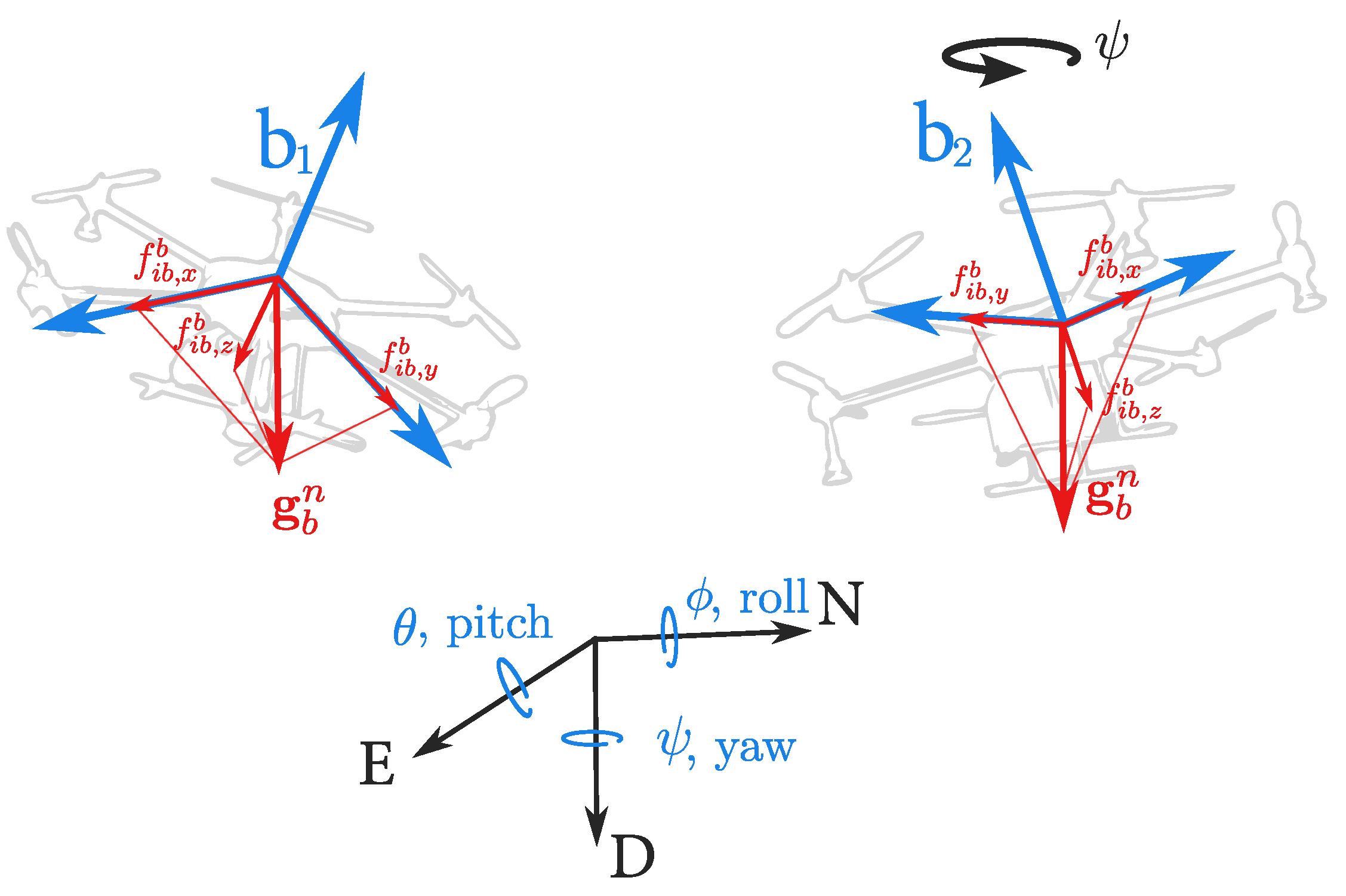
2. Inertial Navigation System for Drones

To achieve an accurate solution to the navigation problem of the UAV platform, the usual approach is to employ a Kalman-like filter to combine GNSS low-frequency measurements with high-frequency IMU-MEM measurements. In particular, our scenario considers that the UAV platform is mounted with a GNSS receiver compatible with RTK processing, such that the filter can update the predicted PVA state variables with highly accurate position measurement. The Kalman filter can adequately yield satisfactory results if the initial pose and sensor bias estimation are accomplished successfully on the ground with reasonable accuracy, depending upon the precision required for the UAV mission. Although static leveling methods can adequately estimate pitch and roll angles in the ground, the heading angle of the drone remains to be determined when the IMU cannot measure the Earth’s rotation. Moreover, ground roll and pitch angles are not so critical since they are well observed by the filter and corrected during the flight without trouble.

While the drone is still before taking flight, the biases of the IMU sensors can be well estimated by the same stochastic filter feed with Zero-Velocity-Updates (ZVU). During this period of pre-tuning, the bias estimation converges, and afterward, the filter parameters switch to the calibrated flight mode. If the drone flight is short, the bias fluctuations will be insignificant and incapable of obliterating the quality of the estimation during the flight. In other words, in short flights, the heading’s initial orientation of the drone is the main problem; for longer flights, bias re-estimation, and heading orientation are both challenges to be carried out. This scenario, combined with any fine adjustments of mechanical parameters of the UAV platform, such as the lever arm or IMU-to-body orientation, motivates the extension for multivariable parameter alignment of our proposed method.

notation: The following notation is adopted: $x_{\beta \alpha }^{\gamma }$ for a vector, x represents the coordinates of some kinematic property (position, velocity, etc.) of frame $\alpha$ w.r.t. frame $\beta$, expressed in frame $\gamma$. The navigation frame is the North-East-Down (NED) local-level frame, abbreviated by the index n; the body frame is indicated by b, the inertial frame by i, whereas the Earth Centered Earth Fixed (ECEF) frame is indexed by e.

2.1. Dynamic and Measurement Models

The PVA kinematic navigation equations in continuous time are given as [3,4],

$$\begin{array}{cc}\hfill {\dot{C}}_b^e& =C_b^e{\left[{\omega }_{ib}^b\right]}^{\times }-{\left[{\omega }_{ie}^e\right]}^{\times }{C}_b^e,\hfill \end{array}$$

(1a)

$$\begin{array}{cc}\hfill {\dot{p}}_{eb}^e& =v_{eb}^e,\hfill \end{array}$$

(1b)

$$\begin{array}{cc}\hfill {\dot{v}}_{eb}^e& =C_b^e{f}_{ib}^b-2{\left[{\omega }_{ie}^e\right]}^{\times }{v}_{eb}^e+g^e\hfill \end{array}$$

(1c)

where the position $p_{eb}^e={\left[x_{eb}^e{y}_{eb}^e{z}_{eb}^e\right]}^{⊺}$ is coordinated in the Earth-Centered-Earth-Fixed (ECEF) frame, and

$${\omega }_{ie}^e={[{\omega }_{e}cos\left(L\right)0-{\omega }_{e}sin\left(L\right)]}^{⊺}$$

where ${\omega }_e$ is the Earth rotation rate, and L is the latitude; ${\omega }_{ib}^b,f_{ib}^b\in {\mathbb{R}}^3$ are the angular velocity and specific force, respectively. Gravity may be obtained through a gravity model; the simplified model in [5] suffices for our purposes.

In [6], it is pointed out that the INS kinematic model in Equation (1) is exact since there is no model error or uncertainty. The uncertainty in navigation problems comes from the sensors and local gravity anomalies.

Gyroscopes and accelerometers are subject to errors that limit the accuracy at which angular rotations or specific forces are measured. The following simplified inertial sensor models are suitable for achieving reliable results for drone missions with short flights:

$$\begin{array}{cc}\hfill {\tilde{\omega }}_{ib}^b& ={\omega }_{ib}^b+b_g+{\epsilon }_g,\hfill \end{array}$$

(2a)

$$\begin{array}{cc}\hfill {\tilde{f}}_{ib}^b& =f_{ib}^b+b_a+{\epsilon }_a,\hfill \end{array}$$

(2b)

where ${\tilde{f}}_{ib}^b$ and ${\tilde{\omega }}_{ib}^b$ are IMU’s noisy values of the specific force and angular velocity, respectively. ${\epsilon }_g\sim \mathcal{N}(0,{\sigma }_g^2)$ and ${\epsilon }_a\sim \mathcal{N}(0,{\sigma }_a^2)$ form iid white noise sequences and are related to the angular random walk (ARW) and velocity random walk parameters of the IMU. In addition, $b_g,b_a$ are the gyroscope and accelerometer biases, respectively, and the biases are expressed in the body frame. The biases are modeled as random walk processes in the form

$$\begin{array}{cc}\hfill d{b}_g& =B_{g}d{W}_g,\hfill \end{array}$$

(3a)

$$\begin{array}{cc}\hfill d{b}_a& =B_{a}d{W}_a,\hfill \end{array}$$

(3b)

where $W_g$ and $W_a$ are Wiener processes of appropriate dimensions and $B_g$ and $B_a$ are diffusion coefficient matrices associated with the IMU’s bias instability.

GNSS position measurements are provided in differential mode and processed using RKT, which is expressed in the ECEF frame. The INS kinematic model is also expressed in the ECEF, such that the GNSS measurements furnish trajectory updates without coordinate transformation. If a navigation solution is required in the local frame coordinates, one can readily transform from ECEF to NED coordinates (see [3]). In this work, we consider that the hover antenna is shifted from the origin of the UAV body coordinate system, whereas the UAV body origin coincides with the IMU origin.

Therefore, the model for the actual measurement must take into account a lever arm effect to provide a meaningful measurement to feed the Kalman filter, as shown in the following equation:

$$p^{\mathrm{GNSS}}=p_{eb}^e+C_b^e{l}^b+\nu$$

(4)

where $\nu \stackrel{iid}{\sim }\mathcal{N}(0,R)$ is the GNSS noise, assumed to be uncorrelated white noise with covariance R.

2.2. Coarse Alignment: Pitch and Roll Angles

Initialization of the inertial navigation system for drone navigation is crucial in order to achieve accurate navigation results. Before takeoff, while the UAV is steady-still in the ground, the INS measures zero linear and angular velocities besides the biases and noises. Thus, the initial values for the gyroscope biases can be estimated by averaging their measurements during this stationary period. Whereas, the initial position can be accurately obtained by averaging GNSS measurements over a sufficiently long time window.

Furthermore, the “leveling method” [3] can be used to obtain the initial pitch (${\theta }_0$) and roll (${\varphi }_0$) angles. The principle behind the leveling method is that when the INS is stationary, the accelerometer triad only perceives the acceleration of gravity. As a result, from trigonometry, the initial pitch and roll angles can be determined as:

$$\begin{array}{cc}\hfill {\theta }_0& =arctan\left({\displaystyle \frac{{\overline{f}}_{ib,x}^b}{\sqrt{{\left({\overline{f}}_{ib,y}^b\right)}^2+{\left({\overline{f}}_{ib,z}^b\right)}^2}}}\right),\hfill \end{array}$$

(5a)

$$\begin{array}{cc}\hfill {\varphi }_0& ={arctan}_2(-{\overline{f}}_{ib,y}^b,-{\overline{f}}_{ib,z}^b)\hfill \end{array}$$

(5b)

where ${\overline{f}}_{ib,x}^b,{\overline{f}}_{ib,y}^b,{\overline{f}}_{ib,z}^b$ are the average accelerometer output during a time window. Note that one should use the four-quadrant arc tangent function for the roll angle. The accuracy of Equation (5) is limited mainly by the accelerometer biases [4].

Regarding the initial heading alignment for a UAV platform, the gyro-compassing method or a magnetometer compass could be used to determine the initial heading. However, gyro-compassing requires expensive navigation-grade gyroscope sensors capable of measuring the earth’s rotation rate, which, as mentioned before, is not the case with low-cost MEMs-IMU devices. In turn, magnetometers usually fail to attain the required precision besides other hindrances to their use, such as the proximity of electric motors and other electromagnetic devices. Another way is to use multi-antenna GNSS receivers to address the heading alignment problem for a UAV platform. However, this also requires more expensive devices. As a result, we aim to develop a method that relies solely on low-cost MEMs and single antenna GNSS hover receiver for proper initialization of the heading angle, as will be described in the following sections.

2.3. The Kalman Filter and its Role in Qualifying Parameters

The Kalman Filter innovation signal forms a zero-mean uncorrelated Gaussian white noise sequence in the pure linear Gaussian scenario. In practical scenarios, this characterization is obliterated, in general. However, the innovation signal remains a figure of merit for good tuning, as it carries a filter’s ability to make one-step predictions and connects to the filter likelihood [7]. It encounters applications, such as multiple targets tracking [8,9] to create measurement gating using Mahalobis or a similar distance. Filter likelihood is at the heart of other filtering schemes, such as interacting multiple models (IMM) filtering [7,10] or particle filtering [11,12], to mention a few.

For the GNSS/INS integration problem tailored for drone navigations, one can employ filters that account for the rigid body kinematics in different manners, such as based on Euler angles, quaternions, or evolving in matrix Lie groups. The latter is employed in [2] with good results, where an EKF based on Lie groups, developed in [13,14], applies for the loosely coupled integration of GNSS/INS of an actual UAV for an application involving drone-borne DinSAR system. The discrete-time EKF in a Lie group takes the form:

$$\begin{array}{cc}\hfill {\widehat{X}}_{k+1|k}& ={\widehat{X}}_{k|k}{exp}_G^{\wedge }\left({\widehat{\Omega }}_k\right),\hfill \end{array}$$

(6a)

$$\begin{array}{cc}\hfill P_{k+1|k}& =\mathcal{F}{P}_{k|k}{\mathcal{F}}^{⊺}+J_r\left({\widehat{\Omega }}_k\right)Q_k{J}_r{\left({\widehat{\Omega }}_k\right)}^{⊺}\hfill \end{array}$$

(6b)

$$\begin{array}{cc}\hfill K_{k+1}& =P_{k+1|k}{\mathcal{H}}^{⊺}{(R_{k+1}+\mathcal{H}{P}_{k+1|k}{\mathcal{H}}^{⊺})}^{-1}\hfill \end{array}$$

(6c)

$$\begin{array}{cc}\hfill {\widehat{X}}_{k+1|k+1}& ={\widehat{X}}_{k+1|k}{exp}_G^{\wedge }\left(K_{k+1}{\eta }_{k+1}\right),{\eta }_{k+1}=y_{k+1}-h\left({\widehat{X}}_{k+1|k}\right)\hfill \end{array}$$

(6d)

$$\begin{array}{cc}\hfill P_{k+1|k+1}& =(I-K\mathcal{H})P_{k+1|k}{(•)}^{⊺}+K{R}_{k+1}{K}^{⊺}\hfill \end{array}$$

(6e)

where

$$\begin{array}{cc}\hfill \mathcal{F}& :={Ad}_G\left({exp}_G^{\wedge }(-{\widehat{\Omega }}_k)\right)+J_r\left({\widehat{\Omega }}_k\right){\mathcal{C}}_k\hfill \end{array}$$

(6f)

$$\begin{array}{cc}\hfill {\mathcal{C}}_k& :={\displaystyle \frac{\partial }{\partial ϵ}}\left[\Omega \left({\widehat{X}}_{k|k}{exp}_G^{\wedge }\left(ϵ\right)\right)\right]{|}_{ϵ=0}\hfill \end{array}$$

(6g)

$$\begin{array}{cc}\hfill \mathcal{H}& :={\displaystyle \frac{\partial }{\partial ϵ}}\left[h\left({\widehat{X}}_{k+1|k}{exp}_G^{\wedge }\left(ϵ\right)\right)\right]{|}_{ϵ=0},\hfill \end{array}$$

(6h)

see the above-mentioned references for more details on the Kalman filter evolving in Lie Groups. In simple terms, the state of a Kalman filter in a Lie group is a matrix that incorporates the kinematic variables of the navigation system. The implementation of the prediction and update step for the EKF in the Lie group is carried out by replacing the usual addition operation with the exponential map of the Lie group, see (6a)–(6d).

Consequently, $k\to {\widehat{X}}_{k|k}$ is the state estimate that contains the estimate of position, velocity, attitude, and eventually estimates of sensor biases; in addition, $k\to y_k$ are the position measurements provided by the GNSS.

Here, of interest is the innovation process $k\to {\eta }_k$ showing the mean update of the filter, Equation (6d). The process $k\to {\eta }_k$ may differ from an ideal sequence of Gaussian white noise, compromised by bias, time correlation, and other imperfections. Still, it yields the simplest form of filter accuracy grading, suitable for verification, adjustment, and comparison by probing its RMS value.

To illustrate, let us consider two filters, $F\left(p_1\right)$ and $F\left(p_2\right)$, parametrized differently by $p_1$ and $p_2$. Taking into account their respective innovation processes $k\to {\eta }_k^1,{\eta }_k^2$, a simple form of ranking their relative accuracy is to evaluate

$$P_{\mathrm{RMS}}^i={\displaystyle \frac{1}{N_2-N_1}}\sum _{k=N_1}^{N_2}{\left({\eta }_k^i\right)}^2,i=1,2$$

along the same set of data trajectory for a period of time $N_2-N_1$ long enough so that the estimates $P_{\mathrm{RMS}}^i$’ become relevant and converge within the required precision. The best performer is clearly $arg{min}_{1,2}{P}_{\mathrm{RMS}}^i$, even if their innovations may be associated with correlation and bias. However, for all defects, the RMS value of the innovation is a practical indicator of filter performance.

In Section 3, we show how the filter innovation RMS can rank heading initialization for drone navigation systems.

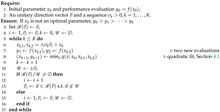
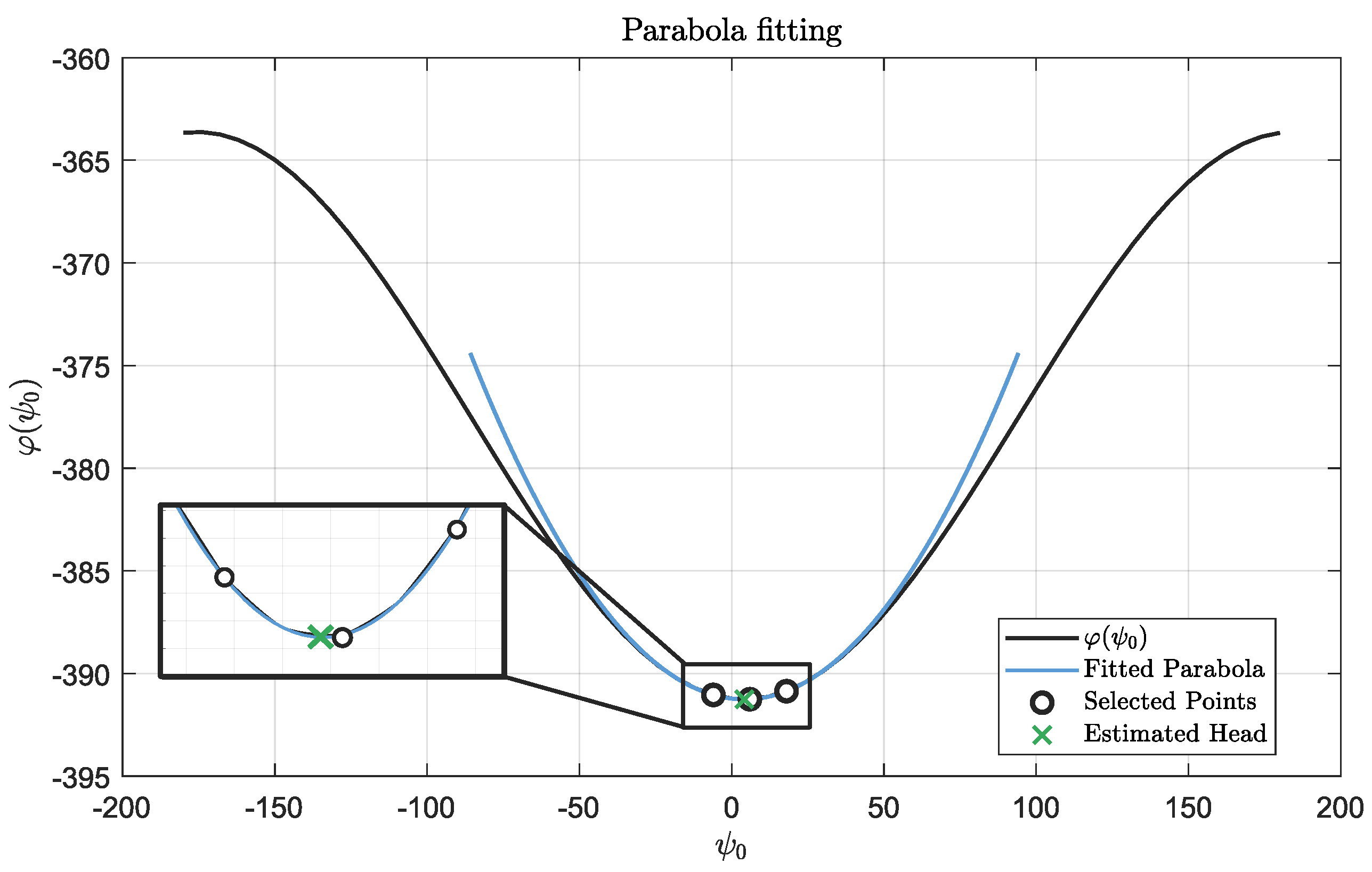
2.4. Unidimensional Quadratic Fit

The last preparatory section presents our primary optimization tool throughout this work. It is the simplest form of finding the minimum of a scalar function without recurring to the gradient1, assuming that the function is unimodal or suffices to find the nearest local minimum. See [15] for the following construction.

Given scalars $x_1,x_2,x_3$ and corresponding values $y_1=f\left(x_1\right),y_2=f\left(x_2\right),y_3=f\left(x_3\right)$, the quadratic function passing through these points is

$$q(x;x_1,x_2,x_3)=\sum _{i=1}^3{y}_i{\displaystyle \frac{{\prod }_{j\ne i}\left(x-x_j\right)}{{\prod }_{j\ne i}\left(x_i-x_j\right)}}.$$

A new point $x_4$ for which the derivative of q vanishes is such that,

$$x_4={\displaystyle \frac{1}{2}}{\displaystyle \frac{b_{23}{y}_1+b_{31}{y}_2+b_{12}{y}_3}{a_{23}{y}_1+a_{31}{y}_2+a_{12}{y}_3}}$$

(7)

where $a_{ij}=x_i-x_j,b_{ij}=x_i^2-x_j^2$. The point $x_4$ is a minimum provided that

$$\sum _{i=1}^3{\displaystyle \frac{y_i}{{\prod }_{j\ne i}\left(x_i-x_j\right)}}>0.$$

(8)

A sequence $x_i,i=1,2,\dots$ is produced by successively applying the quadratic fit above, finding an approximation for the minimum of the original function f as in Equation (7) for $x_4$, and keeping the three out of four points with smaller values of f. Under certain conditions, the sequence is monotonic and converges to the minimum [15].

3. Heading Alignment for UAV

The heading alignment procedure applies differently depending on whether the application is in real-time or post-mission. The more straightforward case is the post-mission one, which will be studied next.

3.1. Post-Mission Heading Alignment

In the post-mission scenario, we seek a reliable initialization of the heading angle (${\psi }_0$) of a UAV platform using the flight track of the drone. Moreover, we are interested in using low-cost MEM sensors without a gyrocompass capability.

For this purpose, we adjust the Bayesian parametric estimation scheme described in (cap. 16 [16]) to the present problem. The method applies when all flight data are collected, represented generically by $y_{1:N}$, and evaluates the posterior distribution $p\left({\psi }_0\right|y_{1:N})$. Once the posterior distribution is obtained, the strategy is to find the most likely value for the initial heading ${\psi }_0$ according to $p\left({\psi }_0\right|y_{1:N})$, which results in the Maximum a Posteriori (MAP) estimator for the initial heading.

To start, note that from Bayes’ theorem, one has

$$p\left({\psi }_0\right|y_{1:N})\propto p\left(y_{1:N}\right|{\psi }_0)p\left({\psi }_0\right)$$

(9)

$p\left({\psi }_0\right)$ is some prior distribution related to a (rough) heading orientation adopted before take-off. For simplicity, consider $\mathbb{E}\left[{\psi }_0\right]=0$ (in degrees or radians) and $p\left({\psi }_0\right)=\mathcal{N}(0,{\sigma }_{\psi }^2)$ as a prior for the heading initial orientation. Moreover, note that $p\left(y_{1:N}\right|{\psi }_0)$ can be factorized in the form

$$p\left(y_{1:N}\right|{\psi }_0)=\prod _{k=1}^{N}p\left(y_k\right|y_{1:k-1},{\psi }_0).$$

(10)

We assume that the marginal measurement distribution $p\left(y_k\right|y_{1:k-1},{\psi }_0)$ is a Gaussian distribution of form

$$p\left(y_k\right|y_{1:k-1},{\psi }_0)=\mathcal{N}(h\left({\widehat{X}}_{k|k-1}^{{\psi }_0}\right),R_k+\mathcal{H}{P}_{k|k-1}^{{\psi }_0}{\mathcal{H}}^{⊺})$$

(11)

where ${\widehat{X}}_{k|k-1}^{{\psi }_0}$ and $P_{k|k-1}^{{\psi }_0}$ come from the filtering solution in Equation (6) associated with some fixed ${\psi }_0$ value. Hence, the most likely value for the initial heading can be found by solving ${min}_{{\psi }_0}-log\left(p\left({\psi }_0\right|y_{1:N})\right)$.

Let $\phi \left({\psi }_0\right)=-log\left(p\left({\psi }_0\right|y_{1:N})\right)$. Then,

$$\begin{array}{c}\phi \left({\psi }_0\right)=\sum _{k=1}^N-log\left(p\left(y_k\right|y_{1:k-1},{\psi }_0)\right)-log\left(p\left({\psi }_0\right)\right)+\mathrm{cte}\hfill \\ \hfill =\sum _{k=1}^N{\displaystyle \frac{1}{2}}log\left(\right|S_k^{{\psi }_0}\left|\right)+{\displaystyle \frac{1}{2}}\parallel {\eta }_k^{{\psi }_0}{\parallel }_{{\left(S_k^{{\psi }_0}\right)}^{-1}}^2+{\displaystyle \frac{1}{2{\sigma }_{\psi }^2}}{\parallel {\psi }_0\parallel }^2+\mathrm{cte}\end{array}$$

(12)

with $S_k^{{\psi }_0}=R_k+\mathcal{H}{P}_{k|k-1}{\mathcal{H}}^{⊺}$ and ${\eta }_k^{{\psi }_0}=y_k-h\left({\widehat{X}}_{k|k-1}^{{\psi }_0}\right)$ is the filter innovation process at time k. Note that for each value of ${\psi }_0$, Equation (12) provides the respective log-likelihood up to a constant such as $p\left({\psi }_0\right|y_{1:N})\propto exp(-\phi \left({\psi }_0\right))$. Thus, for a sufficient number of evaluations of different values for ${\psi }_0$, one can build the distribution $p\left({\psi }_0\right|y_{1:N})$ using the filtering solution.

We also suggest the following approximation $p\left({\psi }_0\right|y_{1:N})\approx \mathcal{N}({\psi }_0^{*},{\sigma }_{{\psi }^{*}}^2)$. The implication is that the log-likelihood should be (approximately) a quadratic function w.r.t. ${\psi }_0$. Hence, by evaluating ${\psi }_0\to \phi \left({\psi }_0\right)$ in three distinct points, one can obtain the approximated log-likelihood function and estimate its minimum using the quadratic fit in Section 2.4.

Therefore, this work proposes a heading alignment scheme well-suited for drone navigation using low-cost MEMs-IMUs sensors consisting of three independent D-LIE-EKF, each with a different initial heading value $\left\{{\psi }_0^1{\psi }_0^2{\psi }_0^3\right\}$. After running these three filters, three samples from the log-likelihood $\phi \left({\psi }_0\right)$ are obtained. After that, an unidimensional quadratic curve is fitted to the samples $({\psi }_0^1,\phi \left({\psi }_0^1\right))$$({\psi }_0^2,\varphi \left({\psi }_0^2\right))$, $({\psi }_0^3,\phi \left({\psi }_0^3\right))$, and a minimizer point ${\psi }_0^{*}$ is determined, see Equation (7). Such a new value may attain precision and suffice to halt the procedure. The quadratic fit approximation improves as the three chosen points are nearer to the minimum; further iterations are a matter of the project’s required accuracy since the quest for the optimal requires producing a minimizing sequence as described in Section 2.4.

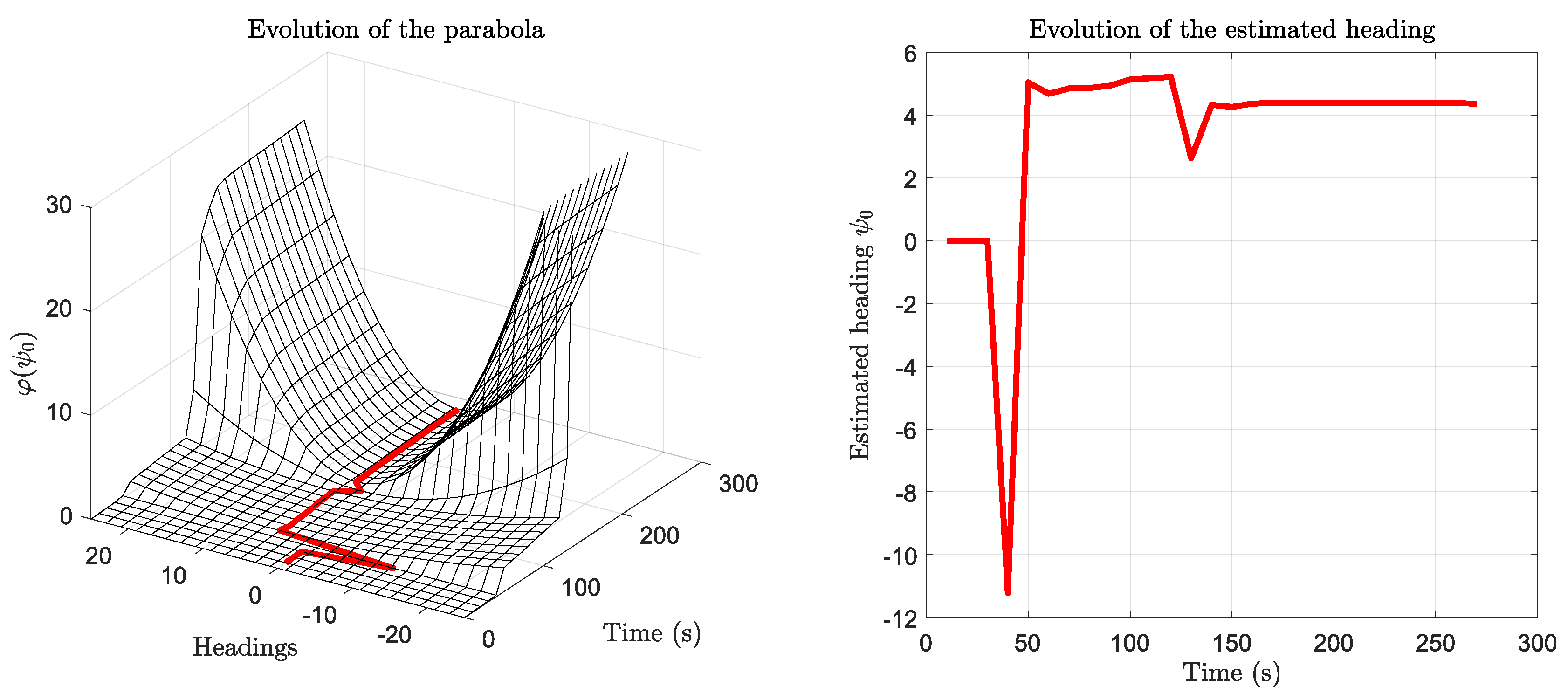
3.2. Real-Time Heading Aligment

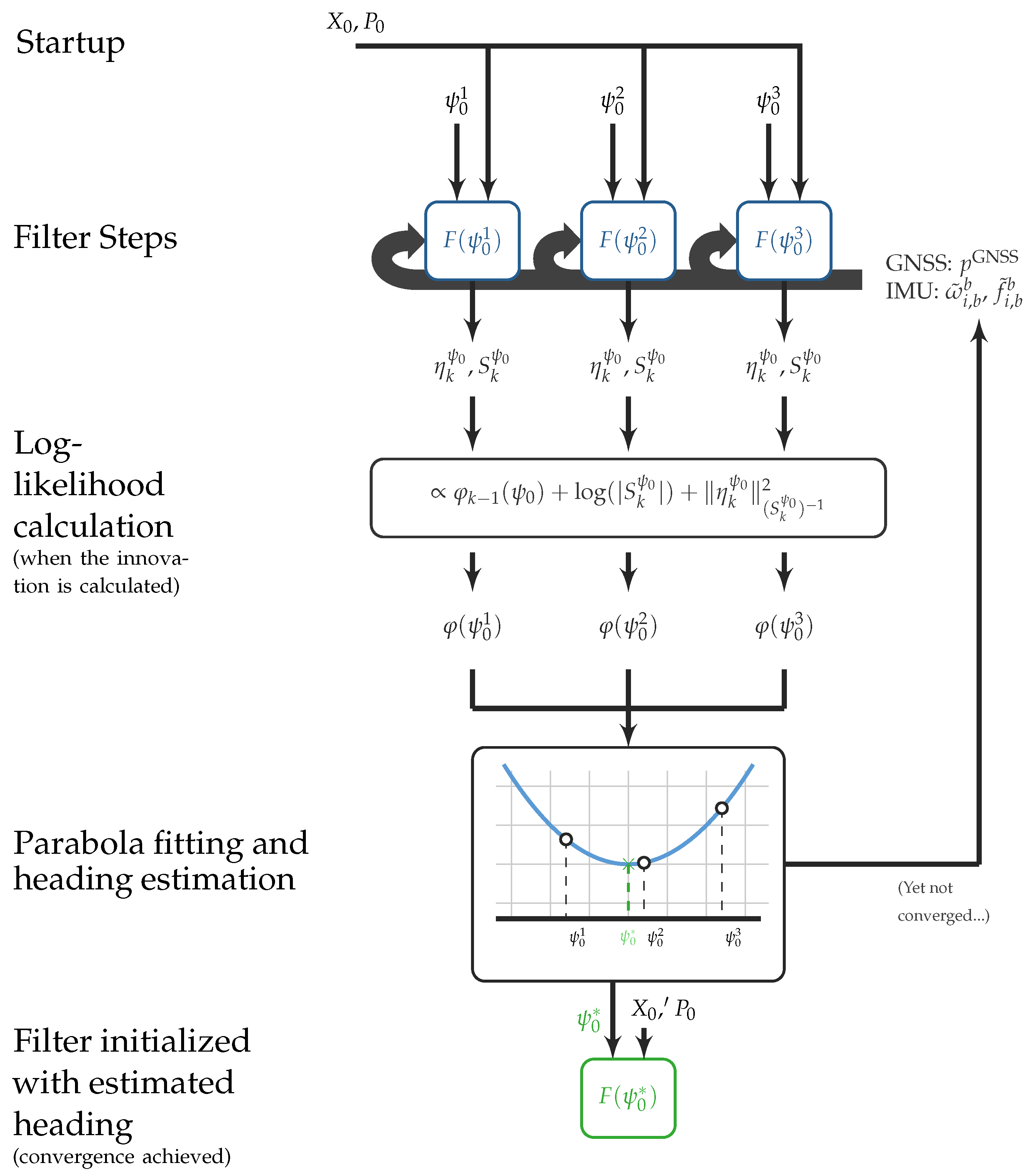
In real-time operations, we devise a procedure to provide initial heading estimates during the actual flight of the drone, allowing an initial time window for a satisfactory estimation. During the calibration window, the following steps are involved; see also Figure 2:

• Initialize a set of three filters ${\left\{F\left({\psi }_0^i\right)\right\}}_{i=1,2,3}$, each parameterized by an initial heading ${\psi }_0^i$ otherwise equal initial conditions. The central value of ${\psi }_0^i$ would carry a rough estimate of the initial heading;
• Acquire streaming data from the GNSS and the IMU. Note that these are obtained at different sampling rates;
• Feed the independent filters with the measurements, executing the prediction step, Equation (6a), at the accelerometer/gyroscope sampling rate, and the update step, Equation (6d), at the GNSS sampling rate;
• During update step, compute for each filter the k-th term of the sum in Equation (12).
• Using the three values of $\phi \left({\psi }_0^i\right)$, parameterize a parabola and find its minimum, representing an estimate of the initial heading ${\psi }_0^{*}$.
• Finally, create a new filter $F\left({\psi }_0^{*}\right)$ initialized with the best initial heading estimate and fed the data collected so far.

After accumulating sufficient values, that is, N in Equation (12) is large enough, the estimate should converge to the initial heading that maximizes the posterior probability, thus, performing a MAP estimation of ${\psi }_0$. A stopping criterion must be adopted to assess convergence, and due to the reduced time to converge, the initial estimation window is small and coincides with initial drone maneuvers.

During the estimation window, one of the three filters considered produces the trajectory estimation Considering the filter processing time, the trajectory estimation provided by the correct filter $F\left({\psi }_0^{*}\right)$ should be able to catch up to the most recent data in the stream.

3.3. Heading Alignment Performance Evaluation

Figure 3 shows an example of a single-step filter-based heading alignment optimization proposed in this work applied to a real navigation dataset collected during an actual flight test of a UAV. It shows the results after convergence during an actual flight mission. Three choices of initial heading angles are ${\psi }_0^1=-6^{\circ },{\psi }_0^2=6^{\circ }$ and ${\psi }_0^3={18}^{\circ }$ are guessed from a rough estimate given by a simple off-the-shelf compass.

The actual log-likelihood curve for ${\psi }_0$ is shown from calculations on a fine angle grid, using 60 distinct initial heading values ranging from $-{180}^{\circ }$ to ${180}^{\circ }$. Near the minimum, a quadratic fit passes through points ${\psi }_0^1,{\psi }_0^2$, and ${\psi }_0^3$ to estimate the precise value. The best initial heading in this example is ${\psi }_0^{*}=4.{38}^{\circ }$. Note that the quadratic approximation is close to the exact curve, and both minima nearly coincide.

The above example corresponds to the post-mission heading alignment operation scenario. In a second experiment, we evaluate the convergence of the method using the same drone flight trajectory now devoted to real-time operation. The result is summarized in Figure 4, depicting how the initial heading value and the quadratic approximation evolve over time.

In an initial stretch, the first 40 seconds of the trajectory, the filter has not yet performed an update step in flight (only ZVU updates), and therefore, no innovation calculation or heading estimation occurs. From the end of this interval, the in-flight update step execution begins, and the heading starts to be estimated.

In the second time stretch, roughly between 100 and 130 seconds, the method does not provide an accurate estimate. The fluctuation of the estimate is large due to the low curvature of the parabola associated with large distribution variances.

Finally, after about 130 seconds (90 seconds from the start of the flight), the initial heading estimate converges to a value of ${\psi }_0^{*}=4.{38}^{\circ }$. At this point, the curvature of the parabola is significantly higher.

4. Extension to Multidimensional Alignments

Here, we call multidimensional alignments in analogy with the scalar case. The idea is to extend the problem studied in Section 3 where we wish to evaluate the performance of a filter $F\left(p\right)$ regarding a multidimensional parameter $p\in {\mathbb{R}}^m$.

The motivation relies on dealing with the accelerometer and gyroscope bias. Also, in some situations, the preliminary alignment of pitch and roll described in Section 2.2 cannot be applied or leads to poor results. In some cases, other parameters are necessary before taking off for a UAV platform, such as the IMU-to-Body rotation matrix or the lever arm to the GNSS antenna. Although the scalar method applied to the heading assessment in Section 3 could be applied sequentially by component, a multivariate method that can deal with all parameters simultaneously is desirable for faster determination. We propose extending the scalar method to deal with such a scenario.

4.1. Multidimensional alignment

Suppose that we are dealing with a multidimensional alignment problem of a UAV platform where a parameter $\mathsf{\Theta }\in {\mathbb{R}}^m$ is constant but unknown during the flight. Following the same approach as described before, define the posterior distribution of these parameters as

$$p\left(\mathsf{\Theta }\right|y_{1:N})\propto p\left(y_{1:N}\right|\mathsf{\Theta })p\left(\mathsf{\Theta }\right)$$

with prior $p\left(\mathsf{\Theta }\right)=\mathcal{N}(0,\Sigma )$. Moreover, note that $p\left(y_{1:N}\right|\mathsf{\Theta })$ can be factorized in the form

$$p\left(y_{1:N}\right|\mathsf{\Theta })=\prod _{k=1}^{N}p\left(y_k\right|y_{1:k-1},\mathsf{\Theta }).$$

(13)

We assume that the marginal measurement distribution $p\left(y_k\right|y_{1:k-1},\mathsf{\Theta })$ is a Gaussian distribution of form

$$p\left(y_k\right|y_{1:k-1},\mathsf{\Theta })=\mathcal{N}(h\left({\widehat{X}}_{k|k-1}^{\mathsf{\Theta }}\right),R_k+\mathcal{H}{P}_{k|k-1}^{\mathsf{\Theta }}{\mathcal{H}}^{⊺})$$

(14)

where ${\widehat{X}}_{k|k-1}^{\mathsf{\Theta }}$ and $P_{k|k-1}^{\mathsf{\Theta }}$ come from the filtering solution in Equation (6) associated with some fixed $\mathsf{\Theta }$ value. Hence, the most likely value for the parameter $\mathsf{\Theta }$ can be found by solving ${min}_{\mathsf{\Theta }}-log\left(p\left(\mathsf{\Theta }\right|y_{1:N})\right)$.

Let $\phi \left(\mathsf{\Theta }\right)=-log\left(p\left(\mathsf{\Theta }\right|y_{1:N})\right)$. Then,

$$\begin{array}{c}\phi \left(\mathsf{\Theta }\right)=\sum _{k=1}^N-log\left(p\left(y_k\right|y_{1:k-1},\mathsf{\Theta })\right)-log\left(p\left(\mathsf{\Theta }\right)\right)+\mathrm{cte}\hfill \\ \hfill =\sum _{k=1}^N{\displaystyle \frac{1}{2}}log\left(\right|S_k^{\mathsf{\Theta }}\left|\right)+{\displaystyle \frac{1}{2}}\parallel {\eta }_k^{\mathsf{\Theta }}{\parallel }_{{\left(S_k^{\mathsf{\Theta }}\right)}^{-1}}^2+{\displaystyle \frac{1}{2}}{\parallel \mathsf{\Theta }\parallel }_{{\Sigma }^{-1}}^2+\mathrm{cte}\end{array}$$

(15)

with $S_k^{\mathsf{\Theta }}=R_k+\mathcal{H}{P}_{k|k-1}{\mathcal{H}}^{⊺}$ and ${\eta }_k^{\mathsf{\Theta }}=y_k-h\left({\widehat{X}}_{k|k-1}^{\mathsf{\Theta }}\right)$ is the filter innovation process at time k. Note that for each value of $\mathsf{\Theta }$, Equation (15) provides the respective log-likelihood up to a constant such as $p\left(\mathsf{\Theta }\right|y_{1:N})\propto exp(-\phi \left(\mathsf{\Theta }\right))$. Thus, for a sufficient number of evaluations of different values for $\mathsf{\Theta }$, one can build the distribution $p\left(\mathsf{\Theta }\right|y_{1:N})$ using the filtering solution.

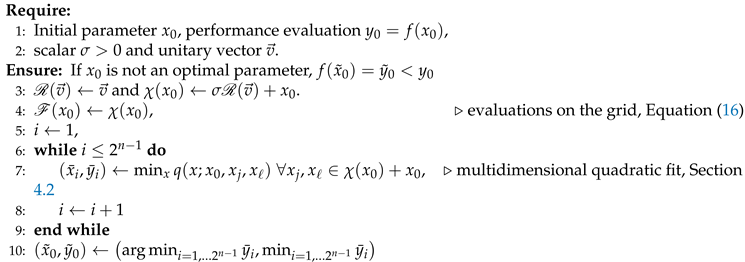
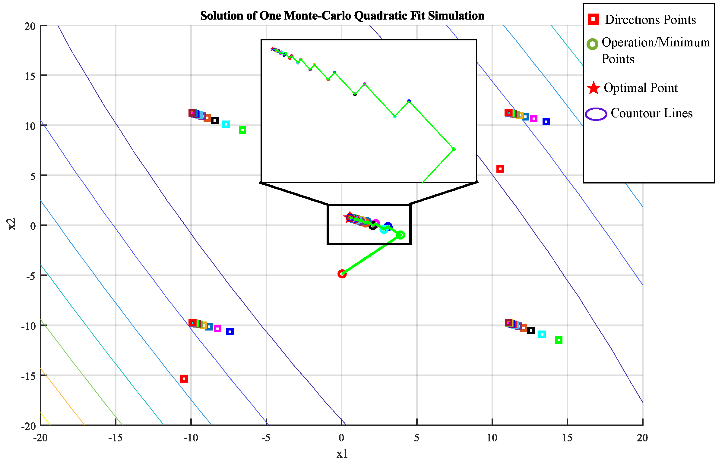
4.2. Quadratic Fit: Multidimensional Extension

Many optimization methods could apply to the multidimensional MAP problem associated with the minimizing $\phi \left(\mathsf{\Theta }\right)$ in Equation (15). Alternatively, the equivalent MMS estimator can be evaluated by sampling the conditional distribution $p\left(\mathsf{\Theta }\right|y_{1:N})$. However, a general feature of the outlined scenarios is that the evaluation until convergence of Equation (15) (or even Equation (12)) at each $\mathsf{\Theta }$ (or ${\psi }_0$) is relatively expensive and depending on the number N that may be large. Besides, attaining the optimal will be costly and perhaps unnecessarily time-consuming, and a procedure that guarantee the monotonicity of the cost, in the sense that $\phi \left({\mathsf{\Theta }}_k\right)>\phi \left({\mathsf{\Theta }}_{k+1}\right)$ whenever ${\mathsf{\Theta }}_k\ne argmin-log\left(p\left(\mathsf{\Theta }\right|y_{1:N})\right)$ is highly desirable.

Considering these constraints, we propose an optimization procedure that applies to the multidimensional case, relying on the simplicity of the quadratic fitting regarding the number of evaluations and the easiness of calculus. First, we brought the linear algebra tools to bear to allow the quadratic fit method to be applied to a multidimensional function using a planar bisection passing through three points.

The problem we wish to unravel is: Given $x_1,x_2,x_3\in {\mathbb{R}}^n$ and the corresponding values $y_1=f\left(x_1\right),y_2=f\left(x_2\right),y_3=f\left(x_3\right)$, find the plane in $(f\left(x\right),x)\in {\mathbb{R}}^{n+1}$ containing these points. If $p_1={\left[y_1{x}_1\right]}^{⊺},p_2={\left[y_2{x}_2\right]}^{⊺}$ and $p_3={\left[y_3{x}_3\right]}^{⊺}$ are the corresponding points in ${\mathbb{R}}^{n+1}$, the plane containing these points can be represent as $\mathcal{P}=\{z\in {\mathbb{R}}^{n+1}:\langle z,\overrightarrow{n}\rangle =c_0$, for some $c_0$, where $\overrightarrow{n}=(p_2-p_1)\times (p_3-p_1)/\parallel (p_2-p_1)\times (p_3-p_1)\parallel$. Applying Givens rotations successively, one obtain a rotation matrix T such that for any $z\in \mathcal{P}$,

$$\left[\begin{array}{c}\alpha \\ \beta \\ 0\\ ⋮\\ 0\end{array}\right]=Tz$$

Applying such transformation to $z_1=0,z_2=p_2-p_1$ and $z_3=p_3-p_1$, we get $T{z}_1=0$ and

$$\left[\begin{array}{c}{\alpha }_2\\ {\beta }_2\\ 0\\ ⋮\\ 0\end{array}\right]=T{z}_2,\left[\begin{array}{c}{\alpha }_3\\ {\beta }_3\\ 0\\ ⋮\\ 0\end{array}\right]=T{z}_3$$

and three coordinate pairs as $({\alpha }_1,{\beta }_1)=(0,0),({\alpha }_2,{\beta }_2)$ and $({\alpha }_3,{\beta }_3)$. Now, by setting the correspondence $(y_1,y_2,y_3)\equiv ({\alpha }_1,{\alpha }_2,{\alpha }_3)$ and $(x_1,x_2,x_3)\equiv ({\beta }_1,{\beta }_2,{\beta }_3)$ in Equation (7), a minimizing value ${\beta }_4$ and the corresponding quadratic value ${\alpha }_4$, provided that Equation (8) is satisfied. From the fact that T is a rotation matrix, thus it is a length preserving transformation, the final result in the original coordinate is obtained by,

$$\left[\begin{array}{c}\sim \\ x_4\end{array}\right]=T^{-1}\left[\begin{array}{c}{\alpha }_4\\ {\beta }_4\\ 0\\ ⋮\\ 0\end{array}\right]+p_1$$

The first component could be the resulting quadratic value if the indicated constant $c_0$ is determined, but it is of no avail in the calculus here.

4.3. The Minimizing Algorithm

A strategy to apply the multidimensional quadratic fit extension in Section 4.2 must be developed. The basic assumption is that the original operating point, say $(x_0,f\left(x_0\right))$, is near the minimum; therefore, the search is local. Also, finding the minimum is not necessarily the goal. One may be satisfied with improving the operating point since seeking the minimum might be time-consuming, computationally expensive, or other practical issues may prevent the quest. Whichever is the reason, the idea is to produce an algorithm to find new operating points while monotonously decreasing costs.

The first notion is to investigate two neighboring points $x_1,x_2$ around $x_0$ and find the corresponding values $y_i=f\left(x_i\right),i=1,2$, apart from the present operating point $(x_0,y_0)$; this represents the most economic spatial covering of the neighborhood of $x_0$. To choose directions $x_1-x_0$ and $x_2-x_0$, we can borrow from curbature integration methods and use the idea of sigma points around $x_0$. Given a unitary norm vector2 $\overrightarrow{v}\in {\mathbb{R}}^n$, create a set of $2^n$ sigma points centered at $x_0$, such as the construction of the set of points is represented by the operator $\mathcal{R}:{\mathbb{R}}^n\to {\mathbb{R}}^{n\times 2^n}$, which applied to $\overrightarrow{v}$ produces a set of ${\mathbb{R}}^n$-valued vectors,

$$\chi \left(x_0\right)=\sigma \mathcal{R}\left(\overrightarrow{v}\right)+x_0$$

containing each combination of $\pi$ rotations componentwisely over $\overrightarrow{v}$. That is, for some unitary $\overrightarrow{v}={\left[\begin{array}{cccc}{v}_1& v_2& \cdots & v_n\end{array}\right]}^{⊺}$, each ${\overrightarrow{v}}_i\in \mathcal{R}\left(\overrightarrow{v}\right)$ has the form ${\left[\begin{array}{cccc}\pm v_1& \pm v_2& \cdots & \pm v_n\end{array}\right]}^{⊺}$ with ${\overrightarrow{v}}_1=\overrightarrow{v}$, together with each of possible distinct signal combinations from $i=2,\dots ,2^n$. Evaluations of the function f on such a grid centered at some $x\in {\mathbb{R}}^n$ are indicated by

$$\mathcal{F}\left(x\right)=f\left(\chi \right(x)+x)$$

(16)

The scalar value $\sigma$ modulates the hypervolume of the sigma-points covering. It relates to the uncertainty of the distance between $x_0$ and the unknown optimal value $x^{*}$. It should be chosen in a way to satisfy $x^{*}\in Co\left(\chi \left(x_0\right)\right)$ preferably, where $Co(·)$ is the convex hull set. Algorithm 1 proceeds with the complete construction and evaluation of the sigma points as the departing idea just described, doing an exhaustive search using $x_0$ as a central point at each performed quadratic fit.

Algorithm 1 A complete step of sigma-point evaluations

The proposed Algorithm 1 is conceptually interesting. Still, it is clearly inefficient since a new minimum, say $x_4$ is found along one direction at each three-point evaluation, and point $x_4$ can play the role of a new central point more efficiently than $x_0$ in Algorithm 1. Since the one-step fit just described produced a monotone decreasing variation, namely $f\left(x_0\right)\ge f\left(x_4\right)$, a variation of Algorithm 1 can be devised to reduce the number of evaluations to attain a better operating point at each step.

Algorithm 2 presents a form that speeds up Algorithm 1 by centering the sigma points at the minimum value at each quadratic fitting step. It again involves a direction is given by a unitary $\overrightarrow{v}$ together with the corresponding “sigma points directions” constellation, ${\overrightarrow{v}}_i\in \mathcal{R}\left(\overrightarrow{v}\right),i=1,\dots ,2^n$, as follows. Given an operation point $x_k$ and a direction ${\overrightarrow{v}}_i$, at each new step, it employs two sigma points symmetrically displaced concerning $x_k$, say $x_{k,1},x_{k,2}=\pm {\sigma }_k{\overrightarrow{v}}_i+x_k$, thus requiring two new evaluations only. Next, the constellation is re-centered at the newly found minimum, and a new direction ${\overrightarrow{v}}_j\in \mathcal{R}\left(\overrightarrow{v}\right)$ is explored, distinct from any of the previously explored.

Note that the total number of sigma points directions are exhausted after $2^{n-1}$ iterations (i.e., $K>2^{n-1}$ in Algorithm 2), and the choice of directions should restart anew. Moreover, with an eye to parsimony, the number of sigma points can be further reduced for the purpose here. It seems enough to explore $2n$ unitary vectors in n orthogonal directions in a n-dimensional parameter space, and if $K=n$ the whole set of directions is examined, namely $\mathcal{R}\left(\overrightarrow{v}\right)/\mathcal{U}\equiv \varnothing$ in Algorithm 2. Lastly, the dispersion parameter $\sigma$ in Algorithm 1 is substituted by a sequence $\left\{{\sigma }_k\right\}$, to express the decreasing distance to the optimal, if one can avail.

Algorithm 2 A stepwise decreasing algorithm

To illustrate the operation of Algorithm 2, a Monte Carlo simulation was performed, in which the following elements at each sample were randomly generated: the optimal parameter value $x^{*}$ and a positive definite matrix such that the cost is $f\left(x\right)={(x-x^{*})}^{⊺}M(x-x^{*})$.

The matrix M is defined by a set of nonnegative eigenvalues, $\lambda \in {\mathbb{R}}^n,{\lambda }_i>0$, in which half of the eigenvalues range between $0.1$ and 10, and a half between 10 and 160. Another support random symmetric matrix provides the orthogonal eigenvectors. The reason for generating eigenvalues with different intervals is to include scenarios where the quadratic form defining f is ill-conditioned. The initial operating point $x_0$ is also randomly generated.

The vector $\overrightarrow{v}$ is chosen as one of the coordinate directions and ${\sigma }_k=5\sqrt{2},\forall k$. As in Algorithm 2, once a minimum is computed, the operating point is re-centered, and the next orthogonal direction is adopted to the minimizing algorithm. Table 1 shows the average relative gain from the initial cost produced by some number of iterations of Algorithm 2. Figure 5 shows convergence towards the minimum in an ill-conditioned case.

Table 1 shows that the minimization method for the 2D case achieves, on average, a relative gain above 99% in 50 iterations, whereas the 6D case requires twice as many iterations to reach the same percentage gain. As expected, this is mainly due to the dimensional number, as a larger number of directions must be assessed ($2^{6-1}=32$ in 6D against 2 directions in 2D), leading to an extended convergence effort to reach the optimal.

Figure 5 depicts the convergence path in an ill-conditioned problem, exhibiting a long zigzag pattern. The minimization process is expected to converge much faster when the Hessian matrix of an actual cost f near the optimal provides a well-conditioned positive quadratic form.

5. Conclusions

The paper studies a technique to improve heading alignment applied to the GNSS/INS integration scenario tailored for drone navigation problems using low-cost MEMs-IMU sensors. It also accounts for multidimensional parameter alignment, resulting in better accuracy of the overall navigation solution for a UAV platform.

It develops a parameter estimation scheme called parameter alignment, which differs from traditional estimation methods. It relies at any time on three identical stochastic filters, except for some initial parameter (or parameter vector). Bayesian analysis produces the metric in Equation (12) that makes a qualifying measure of each filter’s innovation process when monitored over time. The unidimensional quadratic fit applies straightforwardly to these measures under the assumption of the Gaussian posterior distribution, pointing out the optimal value. The work also presents an extension to the multidimensional case, in which the optimization could be done in different manners. In particular, we outline an optimization procedure based on the quadratic fit that improves the parameter alignment value at each step and is well suited to the scenario we explore here. Numeric experiments using synthetic data demonstrate the proposed method’s applicability to finding the initial heading for a drone navigation system. In addition, using the actual dataset from UAV missions, we show that better performance can be achieved in real applications of drone navigations where the IMU is incapable of gyro-compassing. Therefore, the method proposed in this work appears to be a reasonable alternative for low-cost drone navigation systems. Moreover, as far as the authors know, it is a new approach to the initial heading alignment problem that is well suited for the navigation of UAV platforms.

References

1. Gade, K. The Seven Ways to Find Heading. Journal of Navigation 2016, 69, 955–970. [Google Scholar] [CrossRef]
2. Fernandes, M.R.; Magalhães, G.M.; Zúñiga, Y.R.C.; do Val, J.B.R. GNSS/MEMS-INS Integration for Drone Navigation Using EKF on Lie Groups. IEEE Transactions on Aerospace and Electronic Systems 2023, 59, 7395–7408. [Google Scholar] [CrossRef]
3. Groves, P.D. Principles of GNSS, Inertial, and Multisensor Integrated Navigation Systems; Artech House, 2013.
4. Titterton, D.; Weston, J. Strapdown Inertial Navigation Technology, 2nd ed.; The Institution of Electrical Engineers, 2004.
5. Rogers, R.M. Applied Mathematics in Integrated Navigation Systems, 2nd ed.; American Institute of Aeronautics and Astronautics, Inc., 2003.
6. Goel, A.; Aseem, S.; Islam, U.L.; Ansari, A.; Kouba, O.; Bernstein, D.S. An Introduction to Inertial Navigation From the Perspective of State Estimation. IEEE Contr Syst Mag 2021, 45. [Google Scholar]
7. Bar-Shalom, Y.; Li, X.R.; Kirubarajan, T. Estimation with Applications to Tracking and Navigation; Wiley-Interscience, 2001; p. 584.
8. Blackman, S.; Popoli, R. Design and Analysis of Modern Tracking Systems; Artech House Publishers, 1999; p. 1230.
9. Streit, R.; Angle, R.B.; Efe, M. Analytic Combinatorics for Multiple Object Tracking; Springer International Publishing AG, 2020.
10. Blom, H.; Bar-Shalom, Y. The interacting multiple model algorithm for systems with Markovian switching coefficients. IEEE Transactions on Automatic Control 1988, 33, 780–783. [Google Scholar] [CrossRef]
11. Ristic, B.; Arulampalam, S.; Gordon, N. Beyond the Kalman Filter; Artech House Publishers, 2004; p. 318.
12. Chopin, N.; Papaspiliopoulos, O. An Introduction to Sequential Monte Carlo; Springer, 2020; p. 350.
13. Bourmaud, G.; Mégret, R.; Giremus, A.; Berthoumieu, Y. Discrete extended Kalman filter on Lie groups. In Proceedings of the 21st EUSIPCO, Marrakech, Morocco, 2013.
14. Bourmaud, G.; Mégret, R.; Giremus, A.; Berthoumieu, Y. From Intrinsic Optimization to Iterated Extended Kalman Filtering on Lie Groups. J Math Imaging Vis 2016, 55, 284–303. [Google Scholar] [CrossRef]
15. Luenberger, D.G. Introduction to linear and nonlinear programming; Addison-Wesley: Reading, Mass., 1973.
16. Särkkä, S. Bayesian filtering and smoothing, second edition ed.; Number 17 in Institute of Mathematical Statistics textbooks, Cambridge University Press: Cambridge, 2023.
1
Or, for that matter, to the derivatives in general, which may or may not exist.
2
The vector notation is used here to facilitate the understanding.
Figure 1. The diagram illustrates the invariance of the projections of the gravity vector ( f i b , x b , f i b , y b , f i b , z b ) on the body axes of a UAV after a change in the initial heading (yaw rotation). Thus, even before the flight, the readings would be the same for frames b 1 and b 2 , making it impossible to determine the initial heading of the UAV.
Preprints 143528 g001
Figure 2. Illustrative diagram showing the steps involved in obtaining the heading estimate via MAP of p ( ψ 0 | y 1 : N ) in a real-time application of a drone navigation system.
Preprints 143528 g002
Figure 3. Example of the quadratic approximation (blue curve) obtained by sampling three distinct initial heading values. The black curve is the log-likelihood function obtained for a real data flight and filter experiment. Note the remarkable precise sinusoidal profile. The minimum point of the quadratic approximation (in green) is taken as the estimate for the initial heading.
Preprints 143528 g003
Figure 4. Two perspectives following the evolution of heading estimation: the first is a three-dimensional mesh representation of the parabolas fitted over time; the second is a view of the ψ 0 vs. time plane, illustrating the evolution of the estimated heading values (the parabola’s minimum point).
Preprints 143528 g004
Figure 5. path convergence of Algorithm 2 in a ill-conditioned problem in two dimensions.
Preprints 143528 g005