
Submitted:
04 January 2025
Posted:
06 January 2025
You are already at the latest version
Abstract
Background: Causal effect estimates are being used increasingly in medical research-based decision-making. When estimating causal effects from observational studies, methods that can provide sufficient adjustment for confounding are crucial. Clustering structure in observational data and related imbalances across groups (i.e., varying cluster sizes) can present further challenges in statistical analyses and may require appropriate methods or adjustments for accurate inference. Objectives: This study aimed to evaluate the performance of methods for estimating causal effects for binary outcomes in the presence of unbalanced clustered data. Methods: We compared various propensity score-based causal inference approaches including propensity score matching and propensity score weighting methods including those appropriate for clustered data. Using simulation, we assessed the performance of the methods in estimating the average treatment effect on the exposed units under different effect sizes, Intra-Class Correlation (ICC) levels, outcome response surfaces, levels of imbalance, and confounding conditions. Results: In the relatively simple scenario of small effect sizes, under low ICC conditions with no imbalance, both cluster-unconscious (i.e., methods that ignore clustering) and cluster-aware approaches provided similar estimates, even under the presence of some unobserved cluster-level confounding. Otherwise, the bias and precision of estimators appeared to be dependent on levels of ICC, imbalance, and confounding conditions. Additionally, a non-parallel response surface increased bias in the assessed estimators. No single estimator performed better across scenarios, i.e., the accuracy and level of bias appeared to be situation dependent. Conclusion: Both cluster-unconscious and cluster-aware approaches provided similar estimates of the causal effects under relatively simplistic scenarios but procedures that allow for clustering structure would be necessary when the outcome ICC is high, the cluster sizes vary and we cannot rely on the assumption of no unobserved cluster-level confounding. Sample size and power calculation should also account for possible imbalance in cluster sizes, for example, by considering the coefficient of variation at the trial design stage in addition to ICC which is the standard in CRTs.
Keywords:
Causal estimate
; Observational studies
; Clustered data
; Unbalanced cluster sizes
; Propensity score methods
; Intra-class correlation
; Effect size
Introduction
In healthcare research, randomized clinical trials (RCTs) are considered to be the most reliable method for evaluating the efficacy of different healthcare interventions [1]. Randomisation aims to asymptotically balance participant characteristics (observed and unobserved) across exposure levels, allowing causal attribution of differences in outcomes to exposure status. Unfortunately, randomized experiments are not always available because they may be expensive, not feasible, unethical, or just untimely to support an urgent decision[2]. Thus, researchers resort to quasi-experiment/observational study design to assist decision making in medical research which are predominant in health and social science research. Given the continued reliance on this design and the inherent challenge to evaluation of causality in such studies, researchers have increasingly sought methods to improve the estimation of effects from a program or treatment or exposure[3]. Causal inference methods aim to algorithmically randomize individuals. However, even in randomised experiments, the estimation of causal effects is inherently a comparison of potential outcomes (POs) [4]. In the situation of a binary exposure, every individual has two POs: the PO under treatment and the PO under control condition. The PO of an individual is the outcome if individual receives the treatment or not. However, for every individual, we can observe only one of these POs, because each unit (every individual at a specific point in time) will receive either the active treatment (T=1) or the control treatment (T=0), but not both. The unobserved outcome is often referred to as the counterfactual outcome [5]. The estimation of causal effects is like a missing data problem [6], as the PO under the alternative treatment/exposure state cannot be observed; this is sometimes referred to as the fundamental problem of causal inference[7]. Thus, to estimate the effect of the treatment, one needs to identify the counterfactual outcome for the individuals and doing so requires some assumptions.
Most of the methods to identify the causal effect of a non-randomized exposure rely on some causal assumptions which are mostly untestable. The most common assumptions are: Stable Unit and Treatment Version Assumption (SUTVA), consistency, ignorability, and positivity. SUTVA involves two assumptions: (1) no interference which means that units do not interfere with each other and treatment assignment of one unit does not affect the outcome of another unit, and (2) there is one version of the treatment. The consistency assumption implies that the PO under treatment , , is equal to the observed outcome if the actual treatment received is Ignorability, sometimes referred to as the ‘no unmeasured confounding’ or unconfoundedness assumption, implies that given observed pre-treatment characteristics (confounders), treatment assignment is independent from the PO. That is, among units with the same values of the prognostic factors or risk factors (X), we can think of treatment T as being randomly assigned. The positivity assumption essentially states that, for every set of values of X, treatment assignment was not deterministic: , for all t and x. If for some values of X, the treatment assignment was deterministic, then we would have no observed values of Y for one of the treatment groups for those values of X. Variability in the treatment assignment is important for identification. All these assumptions are untestable except for the positivity assumption.
Most existing causal inference methods assume ignorability of treatment assignment mechanism and require fitting two models, one for the assignment mechanism and one for the response surface [8]. Propensity score (PS) based methods, e.g., propensity score matching (PSM) and propensity score weighting (PSW) methods are examples of such strategies. They are less parametric approaches as compared to regression methods [9,10] and take regression estimates of either the propensity function or the response surface (or both) as inputs. Thus, advances in predictive modeling has the potential to improve causal effect estimation using these strategies [11]. Consequently, those strategies are sensitive to misspecification. Defining the wrong causal structure, adjusting for the wrong variables, and omitting a confounder are types of misspecifications that can lead to inaccurate causal effects estimates [12].
Another challenge in estimating causal effects stems from observational data with clustering structure [10]. Clustered data are ubiquitous and statistical procedures for such data may leverage the clustering structure to achieve more accurate estimate. Our choice of models ranges from models that ignore clustering to those that account for clustering. This choice could also be guided by clustering structure and its importance. While clustering structure is related to cluster size and number of clusters, the clustering importance is related to intra-class correlation (ICC) which measures the dependency between units within the same cluster. Clustering can be considered a central or incidental feature of the design [13]. In the first, individual share common and fundamental characteristics while in the second individuals are grouped simply by coincidence. While we expect the ICC to be negligible in incidental setting, it can be important when clustering is central to the design. Procedures that ignore the clustering are prone, among other issues, to cluster-level confounding. Multilevel data structure offers possibilities for several variations on the estimation of average causal effect [9]. Clustering widens the range of model choices in each step of a propensity-score analysis. A range of models from cluster-aware models (mixed effects model, fixed effects model) to cluster-unconscious models can be used to model the treatment assignment mechanism as well as the outcome surface. Furthermore, such grouped data can show imbalances across groups (i.e., varying cluster sizes). Clustered data can be mildly unbalanced (cluster size does not vary much) or highly unbalanced (cluster size has a very high variance); e.g., the cluster size may be 3 or 5 for one cluster while 100 or more for another cluster [14]. Unbalanced cluster size is likely to occur in observational data due to various reasons including missing data and data collection efforts across sites (e.g. hospitals). Even in cluster randomized trial non-uniform dropout would lead to unbalanced cluster size although unlikely to be as severe as it could be in observational data. Imbalance, especially high imbalance can present further challenges in statistical analyses[15] and require appropriate methods or adjustments to account for the imbalance to make accurate inference.
In this study, we aimed to examine the performance of popular propensity score methods in estimating causal effects from unbalanced clustered data. Previous studies have already compared propensity score methods in the context of clustered data[9,16,17] However, there is limited literature examining the impact of cluster imbalance on the estimation bias. The simulation scenarios in Arpino and Cannas (2016)[16] mimic the common situation of unbalanced structure but the authors did not compare the performance of the methods between balanced and unbalanced cluster size settings. In a more extensive simulation, in this study we aimed to investigate the impact of imbalance on model performance considering different levels on imbalance and different average cluster size as well as whether or not the model accounts for clustering. We also assessed the sensitivity of the candidate methods to levels of ICC with the anticipation that methods that ignore clustering will be more sensitive to ICC. Moreover, small effect size could present further challenges for the different estimators; thus, we explored the ability of the candidate methods to uncover small to high effects. As in previous studies[9,16,17], we assessed the sensitivity of the methods to unmeasured cluster-level confounders. Motivated by the simulation design by Hill (2011)[8], we assessed the performance of the candidate models in parallel and non-parallel response surfaces across exposure groups. In contrast to previous studies which tend to simulate continuous outcome [9,17,18], this study has focused on simulating binary outcome. Multi-level data with binary outcome present additional challenges to generalized linear mixed effects models.
Methods
Our study focuses on binary outcomes and complements previous studies which covered primarily continuous outcomes[16]. We put our simulation into the context of research focused on maternal health but the underlying statistical models and related conclusions are applicable to any clustered binary data framework. Thus, let us consider neonatal jaundice within one week as outcome; we are interested in studying the causal association between prematurity and neonatal jaundice. It is crucial to consider confounders that can occur at the baby/women level (individual) and at the hospital level (cluster). For example, at individual-level conditions such as gestational diabetes, preeclampsia, infections, prenatal care, maternal age, mother’s lifestyle, and birth weight are features that are associated to both prematurity and neonatal jaundice. At hospital level, quality of neonatal care, hospital practices for jaundice monitoring, staffing and expertise, hospital volume and resources, and hospital type are important covariates to consider. The general equation of the odds of neonatal jaundice of a baby can be written as follows:
where:
- represents the baseline log-odds of neonatal jaundice;
- represents hospital-specific baseline log-odds of neonatal jaundice and can be viewed as a latent feature that captures hospital’s characteristics, including their practices;
- and are respectively the set of the mother-level and hospitals-level covariates for the baby born in the hospital as mentioned earlier; and quantify how these set of covariates affect the odds of neonatal jaundice;
- represent our main exposure, prematurity and the Log odds-ratio comparing the premature () and non-premature babies ().
In a dataset from different hospitals and described by the data model (1), the baby index runs from 1 to the number of babies in a hospital indexed (). Note that the cluster size is denoted to reflect its variability among hospitals. The hospital-specific baseline log-odds () reflects ICC (i.e., correlation between the outcomes of babies within the same hospital) in the dataset.
With a dataset including clustering structure, there are several methods researchers can choose from (see a review in Chang and Stuart[10]). Considering 20 different candidate methods, we explored various characteristics of clustered data including the mean cluster and standard deviation of the cluster size , and the level of ICC for the binary outcome. We assessed the impact of these cluster characteristics within and between candidate methods while controlling other characteristics such as the association between covariates, the size of the causal effect, and the response surface. Because we simulated the data using equation (1), which assumes the true treatment effect () is known and used to assess the ability of the investigated methods to uncover the true treatment effect. The simulated data is also expected to ensure the ignorability assumption is satisfied and temporality is correct (i.e., outcome after exposure). A brief outline of the investigated simulation scenarios is presented below.
- Intra-class correlation
Within hospital correlation between binary outcomes are introduced by the hospital-specific baseline log-odds (). The random intercept is the realisation of a normal distribution with mean zero and a standard deviation that governs the size of the : . In our simulation we considered three different values: 0.5 (low), 1 (medium) and 1.5 (high) to explore the abilities of the candidate methods under low to high scenarios
- Effect size
Although we are interested in estimating the causal risk difference, we used the log odds-ratio () to control the size of the effect. Two different magnitudes are considered for (0.5 and 2) to investigate the abilities to uncover small and large treatment effects.
- Cluster size
The number of hospitals is assumed to be . In each hospital, the number of deliveries can be influenced by several key characteristics that reflect the hospital’s capabilities, resources, and reputation (for instance, level of maternity care, expertise of medical staff, hospital capacity, referral system, and geographical location). We considered three different mean cluster sizes ( (25, 50, and 100). For each mean cluster size, we explored five levels of cluster imbalance which we controlled with the standard deviation () of cluster size. We considered equal to 0% (perfect balance), 25%, 50%, 75%, and 100% of the average cluster size . For the unbalanced cases, we resorted to the Balanced Discrete Gamma Distribution [19] to generate the cluster sizes () with the restriction .
- Covariates space
We arbitrarily considered 15 covariates. Thus, is a set of five binary covariates and a set of 10 mother-level covariates (five binary and five continuous variables).
- Response surface
We considered parallel and non-parallel response surface across exposure groups (). In the parallel response surface, the partial regression coefficients of the confounders ( and ) were randomly generated from the uniform distribution on independently of the exposure groups. Thus, the potential outcomes were simulated on log-odds scale respectively for non-premature and premature babies as: and . In the non-parallel response surface, were generated separately for non-premature and premature groups as follows: and . The log-odds and are translated into individual probabilities using the inverse logistic link function as . Finally, the probability is used as the parameter of a Bernoulli trial to generate the neonatal jaundice status (outcome) of each baby.
- Prematurity status
Odds of prematurity is computed as: . With and randomly generated using uniform distribution of minimum -1 and maximum 1. With and randomly generated using uniform distribution of minimum -1 and maximum 1. Whereas is the generated as: , resulting in low to moderate ICC in treatment outcome. Then, is translated into individual probabilities using the inverse logistic link function as . Finally, is used as the parameter of a Bernoulli trial to generate the prematurity status (exposure) of each baby
- Candidate methods
We considered propensity score-based methods which have been increasingly used to estimate causal effects when randomization is not available. Propensity score (PS) is defined as the probability of receiving a treatment given the covariates (confounders) characteristics [20]. The PS is a one-dimensional summary of the set of the confounders for the outcome-exposure relationship. In case of a binary exposure, PS can be estimated using a binary logistic regression model where the covariates are the observed pre-treatment characteristics that are associated with the outcome. Those covariates, of course, include the confounders of the outcome-exposure relationship. Once the propensity scores are estimated, there are many ways to use them to estimate the causal effect of the exposure. Propensity score matching (PSM) and propensity score weighting (PSW) are two alternative ways to use propensity score to estimate average treatment effect on treated (ATT). The list of considered candidates methods are presented in Table 1. Throughout this document, we refer to single-level models which do not adjust for clustering as “cluster- unconscious” (C_U). Fixed effect and random intercept models are two model classes that adjust for clustering and referred to as “cluster-aware” (C_A).
- Unobserved cluster-level confounders
To assess the sensitivity of the methods in scenarios where a cluster-level confounders is unobserved, we randomly omitted one variable at a time from after generating the main exposure and the outcome. The importance of omitted cluster-level covariate is measured by the average relative deviation from the true . The true is estimated from single-level logistic regression that account for all the confounders while the “biased” is estimated from a single-level logistic regression that suffer from the omission of one cluster-level confounders.
All scenarios considered for the simulation study involved one of the following combinations: (ICC = Low, Medium, High) x (Effect size = 0.5, 2) x (= 25, 50, 100) x (= 0, 0.25* , 0. 5* , 0.75* , ) x (Confounding = All measured, One unmeasured cluster-level) x (Response surface = parallel, non-parallel).
- Performance metrics
To measure the ability of the different methods to recover the true causal effect, we computed the following performance metrics using 1000 data replicates from each scenario: the relative mean absolute deviation (RMAD), the root mean square error (RMSE), the empirical standard error (SE), and the probability to get an ATT with the same sign as the true causal effect (direction of the estimate).
Results
Our specification of low, medium, and high result respectively in ICC value of [0.02 – 0.04], [0.12 – 0.15], and [0.26 – 0.28], on average. On average = 0.5 produces a risk difference that ranges between -0.08 and -0.6 while = 2 results in a risk difference that ranges between -0.25 and -0.28 which will be referring to these values as true treatment effect under small and large effect size
Figure 1 shows that, irrespective of the method, the deviations of point estimates from the true effect size are symmetrically distributed around zero. This implies that the candidate methods provide unbiased estimates for the true effect. All the candidate methods have also shown lower average relative absolute deviation to uncover a large effect (overall average RMAD = 0.15) as compared to a small effect (overall average RMAD = 0.56) (Figure 2). Figure 3 shows the RMSE values across different average cluster size. It appears that, regardless of the methods, the estimation accuracy improves as the mean cluster size increases from 25 (RMSE ranges from 0.04 to 0.08) to 100 (RMSE ranges from 0.02 to 0.04).
Imbalance: Increased imbalance generally leads to lower accuracy (i.e., higher RMSE) for all methods except the fixed effect model-based PS methods (Figure 4). The double robust methods based on PS estimated from a fixed effect model showed an opposite response, an increased imbalance resulting in a higher accuracy. Interestingly, the effect of imbalance decreases with higher mean cluster size. For example, with imbalance level of 50%, RMSE ranges from 0.05 to 0.08 for mean cluster size of 25 whereas it ranges from 0.02 to 0.04 for mean cluster size of 100.
ICC: Regardless of the method, the RMAD increases as the ICC increases (Figure 5). However, methods that do not account for clustering at any stage have higher elasticity to ICC (Figure 6). For cluster-unconscious methods, the elasticity of the RMAD to ICC ranges from 0.14 to 0.16, i.e., a 1% increase in ICC results on average in 14% to 16% increase in RMAD. In comparison, the elasticity of the RMAD to ICC ranges from 0.03 to 0.12 for cluster-aware methods. Figure 7 shows that the ICC has a larger negative effect on the accuracy (i.e., higher RMSE) of the methods that do not adjust for clustering as compared to cluster-aware methods. Double robust methods based on PS estimated from fixed effect model showed opposite response with increased ICC resulting in higher accuracy.
Unmeasured confounder: Figure 8 shows that the omission of one cluster-level confounder has a small to no effect on the accuracy of all investigated methods including cluster-unconscious methods when the omission does not result in large deviation from , as presented in the table 3. In the scenario depicted in the Figure 8, the relative deviation from the true is 0.22 for low ICC (0.03) and 0.32 for high ICC (0.28). Figure 9 shows the sensitivity of the methods in an exceptional scenario where the omission of cluster confounder results in relatively large deviation (1.46 times away, see Table 3) from . It appears clearly that the accuracy of all cluster-unconscious methods is negatively affected (i.e., increased RMSE). On the other hand, most of the cluster-aware methods are robust to omission of important cluster-level covariate thus, showing little sensitivity.
Direction of causal effect: The performance of the candidate methods in picking the actual (positive or negative) direction of the true effect is presented in Figure 10. For large effect size, irrespective of the ICC level, all the estimators picked the actual direction of the true effect correctly. However, for a small effect size, the probability to pick the right direction ranges from 84.6% to 96.1% under low ICC value, and from 81.6 to 94.6% under high ICC value.
Response surface: The estimation of causal effects appeared to be very sensitive to the presence of an interaction between treatment and covariates (non-parallel response surface) for both small and large effect sizes though with much lower RMAD for the latter (Figure 11). For instance, for small effect size, the RMAD ranges from 0.49 to 0.84 under parallel response surface, and from 2.17 to 2.29 under a non-parallel response surface. Even double robust methods that adjust for interactions between confounders and the exposure variable result in higher deviation from the truth in non-parallel response surface settings as compared to parallel response surface settings.
Table 2 presents a summary of the performance metrics of the cluster-aware and cluster unconscious methods under different conditions of ICC, effect size, imbalance and average cluster size. Cluster-aware methods always have the lowest minimum RMAD, RMSE, and SE but not always the lowest maximum. The overlapping ranges of the performance metrics across cluster-aware and cluster-unconscious estimators indicate that there are techniques adjusting for clustering that do not always result in better performance as compared to techniques ignoring clustering. Table 2 also shows that in general small effect size, high ICC, small mean cluster size, and imbalance are challenging settings for the investigated causal effect estimation methods.

Table 2.
Range of performance metric across cluster-aware and cluster-unconscious methods under parallel response surface.
Table 2.
Range of performance metric across cluster-aware and cluster-unconscious methods under parallel response surface.
| Effect | ICC | CS | Imbalance | Method | Relative bias | RMSE | SE | Direction(%) |
|---|---|---|---|---|---|---|---|---|
| Small | Low | 25 | 0 | C_A | 0.475 - 0.836 | 0.045 - 0.078 | 0.001 - 0.002 | 0.846 - 0.961 |
| C_U | 0.487 - 0.634 | 0.046 - 0.06 | 0.001 - 0.002 | 0.886 - 0.961 | ||||
| 1 | C_A | 0.511 - 0.86 | 0.05 - 0.081 | 0.002 - 0.003 | 0.826 - 0.946 | |||
| C_U | 0.518 - 0.688 | 0.053 - 0.065 | 0.002 - 0.002 | 0.865 - 0.941 | ||||
| 100 | 0 | C_A | 0.246 - 0.399 | 0.024 - 0.038 | 0.001 - 0.001 | 0.978 - 0.998 | ||
| C_U | 0.266 - 0.332 | 0.025 - 0.032 | 0.001 - 0.001 | 0.982 - 0.997 | ||||
| 1 | C_A | 0.249 - 0.4 | 0.024 - 0.038 | 0.001 - 0.001 | 0.971 - 0.998 | |||
| C_U | 0.267 - 0.339 | 0.025 - 0.033 | 0.001 - 0.001 | 0.984 - 0.997 | ||||
| High | 25 | 0 | C_A | 0.528 - 0.966 | 0.044 - 0.08 | 0.001 - 0.002 | 0.813 - 0.946 | |
| C_U | 0.679 - 0.825 | 0.055 - 0.068 | 0.002 - 0.002 | 0.828 - 0.872 | ||||
| 1 | C_A | 0.562 - 0.944 | 0.047 - 0.077 | 0.001 - 0.002 | 0.791 - 0.92 | |||
| C_U | 0.684 - 0.851 | 0.059 - 0.069 | 0.002 - 0.002 | 0.826 - 0.881 | ||||
| 100 | 0 | C_A | 0.269 - 0.449 | 0.022 - 0.037 | 0.001 - 0.001 | 0.961 - 0.998 | ||
| C_U | 0.422 - 0.491 | 0.035 - 0.04 | 0.001 - 0.001 | 0.94 - 0.967 | ||||
| 1 | C_A | 0.268 - 0.431 | 0.023 - 0.036 | 0.001 - 0.001 | 0.95 - 0.997 | |||
| C_U | 0.422 - 0.488 | 0.035 - 0.041 | 0.001 - 0.001 | 0.941 - 0.964 | ||||
| Large | Low | 25 | 0 | C_A | 0.127 - 0.224 | 0.045 - 0.079 | 0.002 - 0.003 | 0.998 - 1 |
| C_U | 0.13 - 0.168 | 0.046 - 0.06 | 0.002 - 0.002 | 1 - 1 | ||||
| 1 | C_A | 0.137 - 0.226 | 0.051 - 0.081 | 0.002 - 0.003 | 0.995 - 1 | |||
| C_U | 0.139 - 0.184 | 0.054 - 0.066 | 0.002 - 0.002 | 0.998 - 0.999 | ||||
| 100 | 0 | C_A | 0.064 - 0.105 | 0.023 - 0.038 | 0.001 - 0.002 | 1 - 1 | ||
| C_U | 0.069 - 0.088 | 0.025 - 0.032 | 0.001 - 0.001 | 1 - 1 | ||||
| 1 | C_A | 0.067 - 0.107 | 0.024 - 0.038 | 0.001 - 0.002 | 1 - 1 | |||
| C_U | 0.072 - 0.09 | 0.026 - 0.032 | 0.001 - 0.002 | 1 - 1 | ||||
| High | 25 | 0 | C_A | 0.141 - 0.256 | 0.045 - 0.081 | 0.002 - 0.003 | 0.997 - 1 | |
| C_U | 0.177 - 0.216 | 0.055 - 0.068 | 0.002 - 0.002 | 1 - 1 | ||||
| 1 | C_A | 0.145 - 0.242 | 0.047 - 0.076 | 0.002 - 0.003 | 0.995 - 1 | |||
| C_U | 0.176 - 0.221 | 0.058 - 0.069 | 0.002 - 0.002 | 0.997 - 0.999 | ||||
| 100 | 0 | C_A | 0.07 - 0.12 | 0.022 - 0.038 | 0.001 - 0.002 | 1 - 1 | ||
| C_U | 0.111 - 0.13 | 0.035 - 0.04 | 0.001 - 0.002 | 1 - 1 | ||||
| 1 | C_A | 0.071 - 0.115 | 0.023 - 0.036 | 0.001 - 0.002 | 1 - 1 | |||
| C_U | 0.115 - 0.13 | 0.036 - 0.042 | 0.001 - 0.002 | 1 - 1 |
CS: Average Cluster size, RMSE: Root mean square error, SE: Empirical standard error, ICC: intra-class correlation, C_A: cluster-aware methods, C_U: cluster-unconscious methods.
Table 3.
Relative deviation from for small effect size.
| Mean Cluster size | Imbalance Level | ICC value | Relative absolute deviation from theta |
|---|---|---|---|
| 25 | 0.00 | 0.03 | 0.22 |
| 0.14 | 0.28 | ||
| 0.28 | 0.32 | ||
| 0.50 | 0.02 | 0.44 | |
| 0.13 | 0.40 | ||
| 0.27 | 0.32 | ||
| 0.96 | 0.02 | 0.17 | |
| 0.12 | 0.29 | ||
| 0.26 | 0.36 | ||
| 50 | 0.00 | 0.03 | 0.13 |
| 0.14 | 0.16 | ||
| 0.28 | 0.29 | ||
| 0.50 | 0.03 | 0.13 | |
| 0.14 | 0.30 | ||
| 0.28 | 0.25 | ||
| 0.96 | 0.03 | 0.12 | |
| 0.13 | 0.25 | ||
| 0.27 | 0.37 | ||
| 100 | 0.00 | 0.04 | 0.11 |
| 0.15 | 0.14 | ||
| 0.28 | 0.24 | ||
| 0.50 | 0.04 | 0.10 | |
| 0.14 | 0.13 | ||
| 0.28 | 0.25 | ||
| 0.96 | 0.03 | 0.10 | |
| 0.14 | 0.17 | ||
| 0.27 | 1.46 |
Table 4 shows the top two most accurate methods (based RMSE) given sample characteristics including ICC, mean cluster size and imbalance level. Cluster-aware methods performed consistently better and demonstrated less sensitivity to ICC.
Discussion
In this study, we assessed the performance of commonly applied methods for estimating the average causal effect of an exposure on a binary outcome from clustered observational (non-randomized) data. The main contribution of this work is an objective evaluation of most available causal effect estimation methods depending on study design and data structure. We investigated the bias and accuracy of the candidate methods considering some measurable characteristics from such data. These characteristics include the level of ICC in the binary outcome, the average size of clusters, and the level of imbalance in cluster sizes. Our results can be considered as a tool in selecting a relatively accurate method given average cluster size, cluster imbalance and ICC. This can guide applied researchers investigating the causal effect of an exposure on a binary outcome in clustered observational data.
Propensity score methods are known to provide unbiased estimates of causal treatment effects in observational designs, provided the underlying assumptions hold[20,22]. Our simulations indicated that all the candidate methods are unbiased. This indicates that popular causal inference methods, irrespective of the use of the cluster-related information available in the data, or the use of fixed effect or random intercept model to derive PSs, do not consistently overestimate or underestimate the true causal effect ,i.e., the estimated causal effect approaches the true effect as the sample size increases.
However, the accuracy of the estimates varied across methods, the best method depending on some characteristics in the data. As demonstrated by a number of studies[9,16] methods that generally perform the best are methods that allow for clustering at least at one stage of the estimation either parametrically or nonparametrically. After ranking, most of the methods that perform the best are consistently double robust methods that adjust for clustering in outcome model either through fixed effect or random intercept model but with . Propensity score models for these methods are from single-level model which suggest that accounting for clustering in treatment assignment mechanism is not as important as it is for outcome model. It should be noted that our simulation limited ICC levels to medium for treatment generation which could justify the suitability of single level model for treatment model.
Thoemmes and West [13] found that ignoring cluster membership can yield relatively accurate results when ICC is small (0.05). We reached a similar conclusion here because, in datasets with a low ICC, estimates from both cluster-unconscious (ignoring clustering structure) and cluster-aware (leverage clustering structure) methods show similar accuracies as measured by RMAD and RMSE. Further, our findings indicate that excluding a single cluster-level confounder does not always significantly impact on the accuracy of the methods being compared when the omitted confounder does not result in substantial deviation from the true odds ratio. Under this circumstance, even cluster-unaware methods demonstrate robustness. However, these methods show clear sensitivity to the omission of relatively important cluster-level confounders, unlike cluster-aware methods, which maintain their robustness even when an important cluster-level confounder is excluded. An interesting finding is that, given some data characteristics such as low ICC certain cluster-unconscious methods outperform cluster-aware methods. This supports the counter-intuitive finding of Scott et al. [18] and Middleton et al. (2016)[23] that ignoring group structure can sometimes lead to estimators with less absolute bias as compared to estimators that account for group structure. This could be related to the low importance of clustering in the treatment assignment mechanism. Otherwise stated, cluster-unconscious methods may have better accuracy than cluster-aware methods when treatment assignment and outcome mechanism are only moderately related to clustering, and no important cluster-level confounder is omitted. High ICC was also showed to affect both cluster-unconscious and cluster-aware methods, but the latter demonstrated lower sensitivity, as expected. Thus, we reckon that the level of ICC can inform the choice of estimation models and confidence in the findings.
One of the main contributions of this study is highlighting the impact of imbalance in cluster sizes on the accuracy of estimates when applying common causal inference methods. Our results demonstrated that imbalance in cluster sizes generally reduces the accuracy of most methods, but the accuracy reduction wanes out with increasing average cluster size. We also found that methods based on PS estimated from a fixed effect model showed a higher accuracy for increased imbalance.
This study also showed that no single causal inference method is uniformly preferable in all situations [18]. Thus our proposed guidance presented in Table 4 for choosing the optimal method can be helpful in the case of binary outcome data with clustering structure. Propensity score matching methods consistently perform worse than propensity score weighting, regardless of whether the propensity scores are estimated from models that account for clustering. However, this may be due to the caliper we used (0.2 of the standard deviation). The use of a caliper can also lead to some individuals being unmatched if no suitable match is found within the specified distance, which is a limitation of this study.
Finally, our study flags the limitation of commonly used regression-based methods to estimate causal effects when the response surface is not parallel across treatment groups. Fuentes et al. (2022)[17] found that when the data were generated with random slopes in the treatment and outcome equations, all the methods that ignore the varying effect of the cluster-level covariate were substantially biased, regardless of the cluster size. Our simulations showed that this results hold in general for varying slopes in treatment groups, independently of the fixed or random slope assumption.
Furthermore, we focused only on the impact outcome ICC while constraining the within-cluster correlation in terms of treatment assignment to only medium (≤ 0.12). Unmeasured cluster-level confounding could otherwise inflate bias if clustering is important for both treatment and outcome. Future investigations can extend our simulation to explore combination of various ICC levels in outcome and treatment assignment.
Supplementary Materials
The following supporting information can be downloaded at the website of this paper posted on Preprints.org
References
- Colli, A., Pagliaro, L. & Duca, P. The ethical problem of randomization. Internal and emergency medicine 9, 799–804 (2014). [CrossRef]
- Hernan, M. & Robins, J. Causal inference: What if. boca raton: Chapman & hill/crc. (2020).
- Guo, S. & Fraser, M. W. Propensity Score Analysis: Statistical Methods and Applications. vol. 11 (SAGE publications, 2014).
- Rubin, D. B. Estimating causal effects of treatments in randomized and nonrandomized studies. Journal of educational Psychology 66, 688 (1974). [CrossRef]
- Sande, G. & Rothman, K. Modern Epidemiology. (1998).
- Rubin, D. B. Inference and missing data. Biometrika 63, 581–592 (1976).
- Holland, P. W. Statistics and causal inference. Journal of the American statistical Association 81, 945–960 (1986).
- Hill, J. L. Bayesian nonparametric modeling for causal inference. Journal of Computational and Graphical Statistics 20, 217–240 (2011). [CrossRef]
- Li, F., Zaslavsky, A. M. & Landrum, M. B. Propensity score weighting with multilevel data. Statistics in medicine 32, 3373–3387 (2013). [CrossRef]
- Chang, T.-H. & Stuart, E. A. Propensity score methods for observational studies with clustered data: a review. Statistics in medicine 41, 3612–3626 (2022). [CrossRef]
- Hahn, P. R., Murray, J. S. & Carvalho, C. M. Bayesian regression tree models for causal inference: Regularization, confounding, and heterogeneous effects (with discussion). Bayesian Analysis 15, 965–1056 (2020). [CrossRef]
- Prosperi, M. et al. Causal inference and counterfactual prediction in machine learning for actionable healthcare. Nature Machine Intelligence 2, 369–375 (2020). [CrossRef]
- Thoemmes, F. J. & West, S. G. The use of propensity scores for nonrandomized designs with clustered data. Multivariate behavioral research 46, 514–543 (2011). [CrossRef]
- Samanta, M. & Welsh, A. H. Bootstrapping for highly unbalanced clustered data. Computational Statistics & Data Analysis 59, 70–81 (2013). [CrossRef]
- W. Van der Elst, V. N., L. Hermans, G. Verbeke, M. G. Kenward & Molenberghs, G. Unbalanced cluster sizes and rates of convergence in mixed-effects models for clustered data. Journal of Statistical Computation and Simulation 86, 2123–2139 (2016). [CrossRef]
- Arpino, B. & Cannas, M. Propensity score matching with clustered data. An application to the estimation of the impact of caesarean section on the Apgar score. Statistics in medicine 35, 2074–2091 (2016). [CrossRef]
- Fuentes, A., Lüdtke, O. & Robitzsch, A. Causal inference with multilevel data: A comparison of different propensity score weighting approaches. Multivariate Behavioral Research 57, 916–939 (2022). [CrossRef]
- Scott, M. A., Diakow, R., Hill, J. L. & Middleton, J. A. Potential for bias inflation with grouped data: a comparison of estimators and a sensitivity analysis strategy. Observational Studies 4, 111–149 (2018). [CrossRef]
- Tovissodé, C. F., Honfo, S. H., Doumatè, J. T. & Glèlè Kakaï, R. On the discretization of continuous probability distributions using a probabilistic rounding mechanism. Mathematics 9, 555 (2021). [CrossRef]
- Rosenbaum, P. R. & Rubin, D. B. The central role of the propensity score in observational studies for causal effects. Biometrika 70, 41–55 (1983).
- D’Agostino Jr, R. B. Propensity score methods for bias reduction in the comparison of a treatment to a non-randomized control group. Statistics in medicine 17, 2265–2281 (1998).
- Middleton, J. A., Scott, M. A., Diakow, R. & Hill, J. L. Bias amplification and bias unmasking. Political Analysis 24, 307–323 (2016). [CrossRef]
- Hirano, K., Imbens, G. W. & Ridder, G. Efficient estimation of average treatment effects using the estimated propensity score. Econometrica 71, 1161–1189 (2003). [CrossRef]
- Horvitz, D. G. & Thompson, D. J. A generalization of sampling without replacement from a finite universe. Journal of the American statistical Association 47, 663–685 (1952).
Figure 1.
Index plot of the deviation of point estimates from the true effect with: small true effect size, low ICC (all confounders accounted for, parallel response surface, and perfectly balanced cluster size (). The shown indices are for 200 simulations randomly sampled from the 1000 replicates for each evaluated method (the red horizontal line represents zero bias). Description and reference for each method is provided in Table 1.
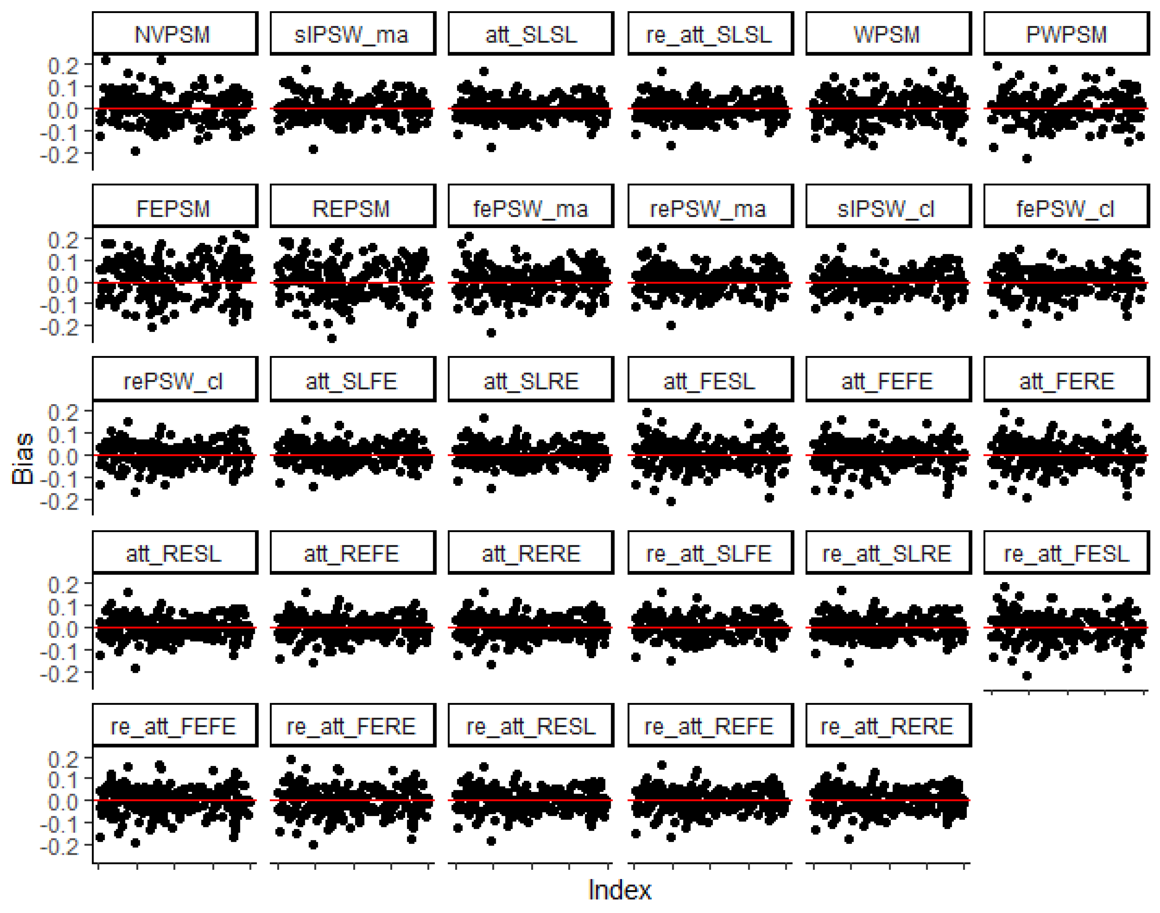
Figure 2.
Average relative absolute deviation from true effect (low ICC, all confounders accounted for, parallel response surface, perfectly balanced clustered size). Blue dots indicate cluster-unconscious methods.
Figure 2.
Average relative absolute deviation from true effect (low ICC, all confounders accounted for, parallel response surface, perfectly balanced clustered size). Blue dots indicate cluster-unconscious methods.
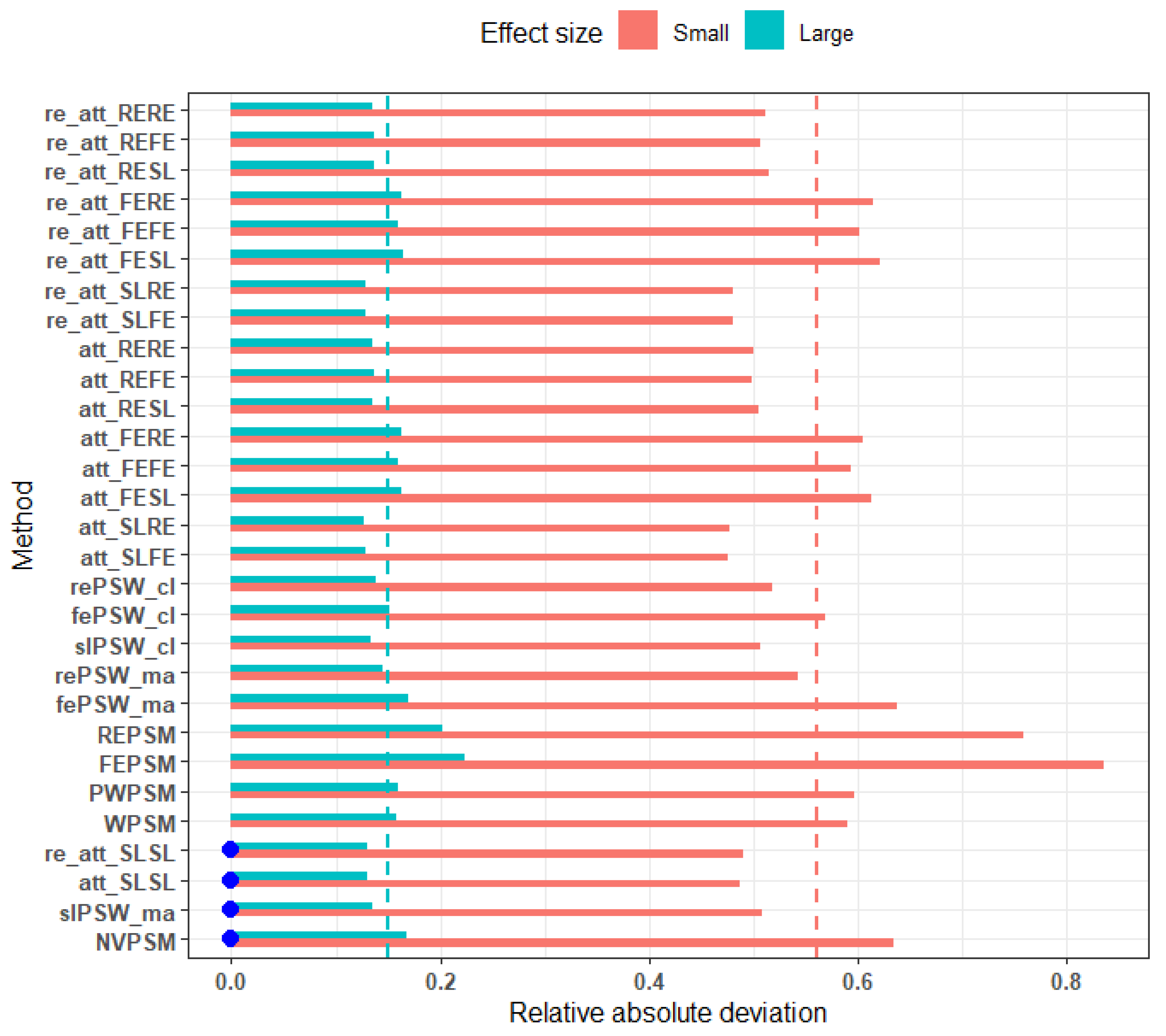
Figure 3.
RMSE across different average cluster size (small effect, perfectly balanced cluster, low ICC, and no unmeasured confounders). Blue dots indicate cluster-unconscious methods.
Figure 3.
RMSE across different average cluster size (small effect, perfectly balanced cluster, low ICC, and no unmeasured confounders). Blue dots indicate cluster-unconscious methods.
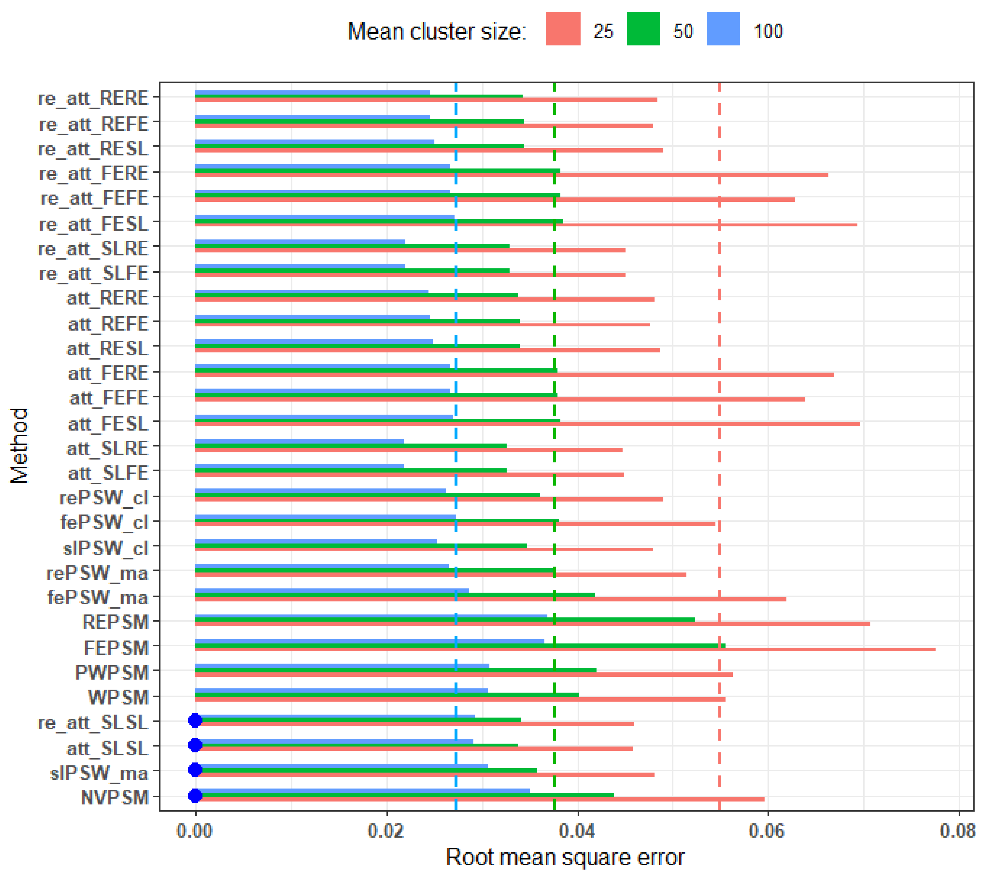
Figure 4.
RMSE of methods across different levels of imbalance and average cluster size: small effect, low ICC, parallel response surface, all confounders adjusted for. Blue dots indicate cluster-unconscious methods. .
Figure 4.
RMSE of methods across different levels of imbalance and average cluster size: small effect, low ICC, parallel response surface, all confounders adjusted for. Blue dots indicate cluster-unconscious methods. .
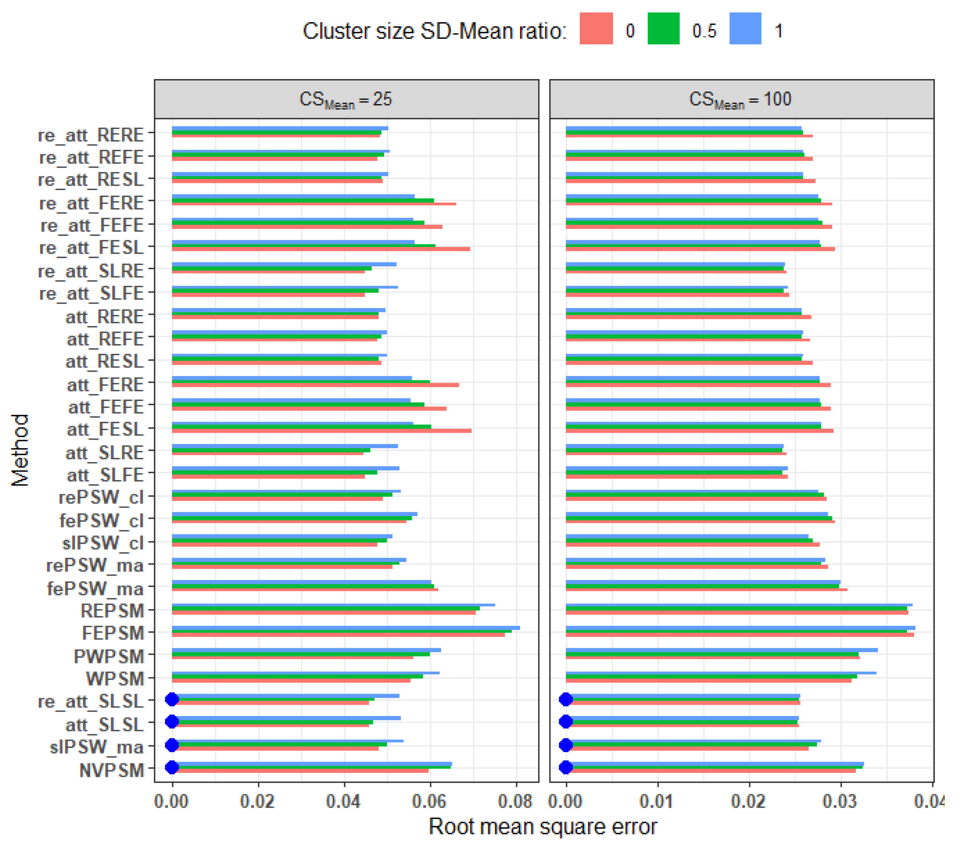
Figure 5.
Relative bias across different level of outcome ICC (all confounders accounted for, parallel response surface, perfectly balanced clustered size). Blue dots mark cluster-unconscious methods.
Figure 5.
Relative bias across different level of outcome ICC (all confounders accounted for, parallel response surface, perfectly balanced clustered size). Blue dots mark cluster-unconscious methods.
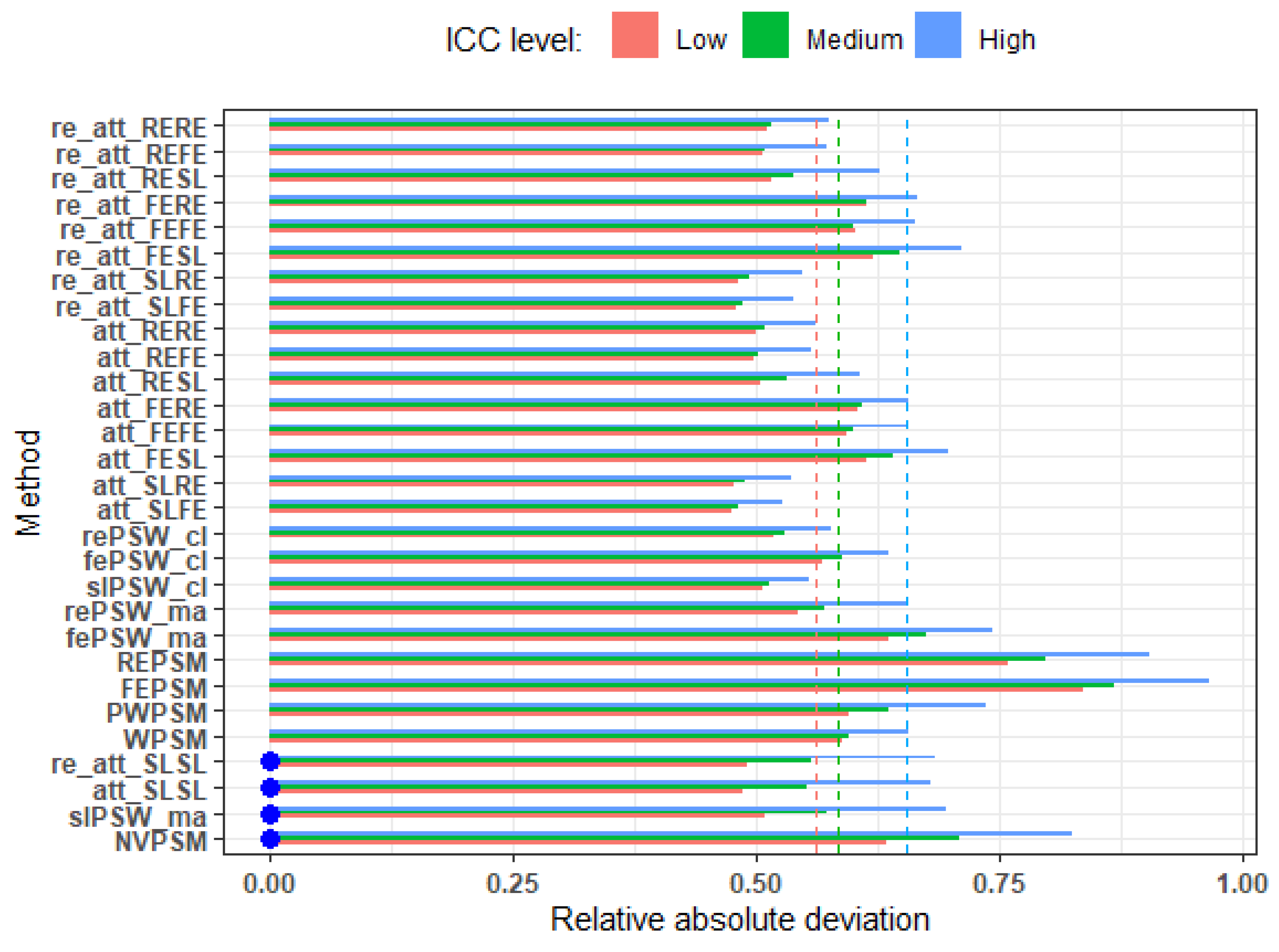
Figure 6.
Elasticity of relative bias against ICC. We regrouped the ICC values across replications into 10 equal size groups and considered the average ICC value within each group. Then we regressed the log (relative absolute deviation) on the log (average ICC). The value in the each plot title is the slope which is the elasticity of the relative bias to ICC. It represents the change the in relative bias associated with 1% change in ICC.
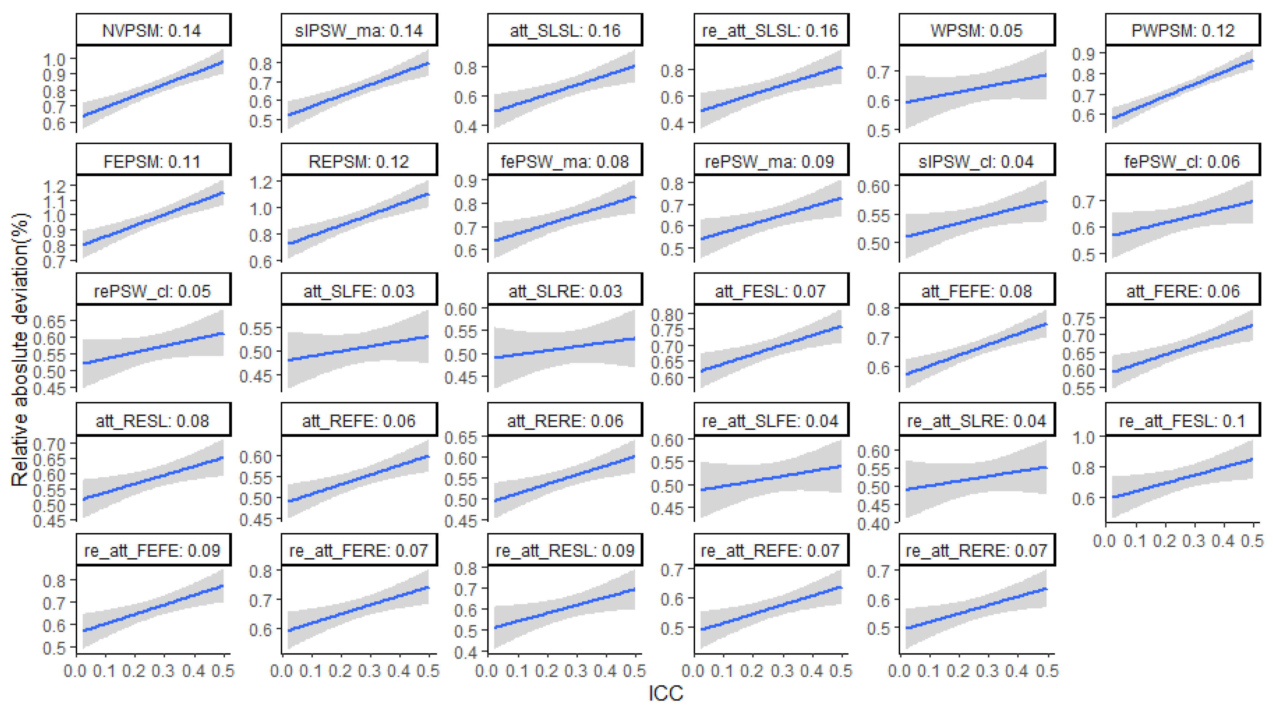
Figure 7.
RMSE across different levels of ICC: average cluster size 25, perfectly balanced, small effect. Blue dots mark cluster-unconscious methods.
Figure 7.
RMSE across different levels of ICC: average cluster size 25, perfectly balanced, small effect. Blue dots mark cluster-unconscious methods.
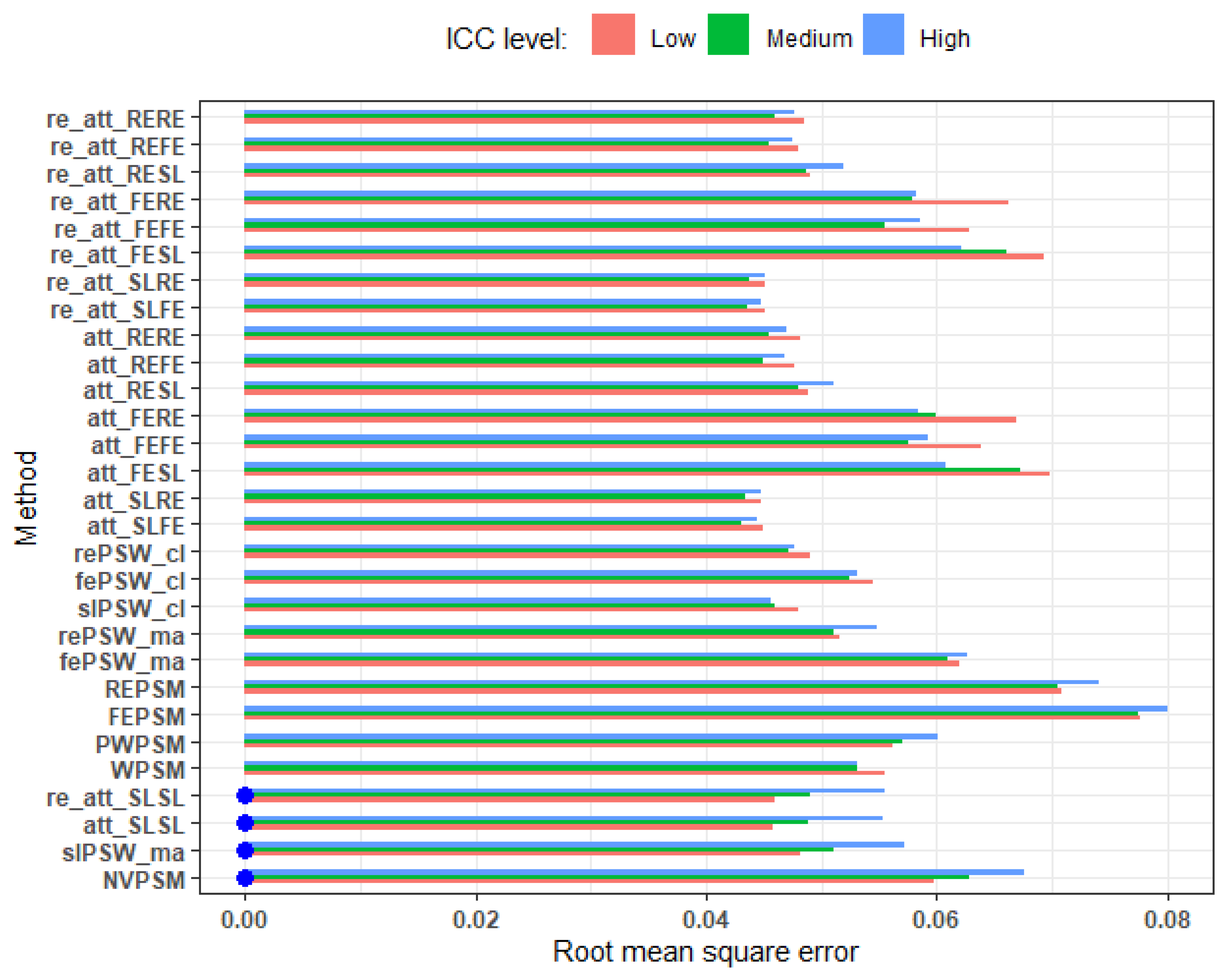
Figure 8.
RMSE comparing scenario where we adjusted for all cluster-level covariates and when there is one unmeasured confounder. Blue dots mark cluster-unconscious methods. Small effect size, average cluster size of 25, parallel response space and perfectly balanced. Relative deviation from less than equal to 0.33.
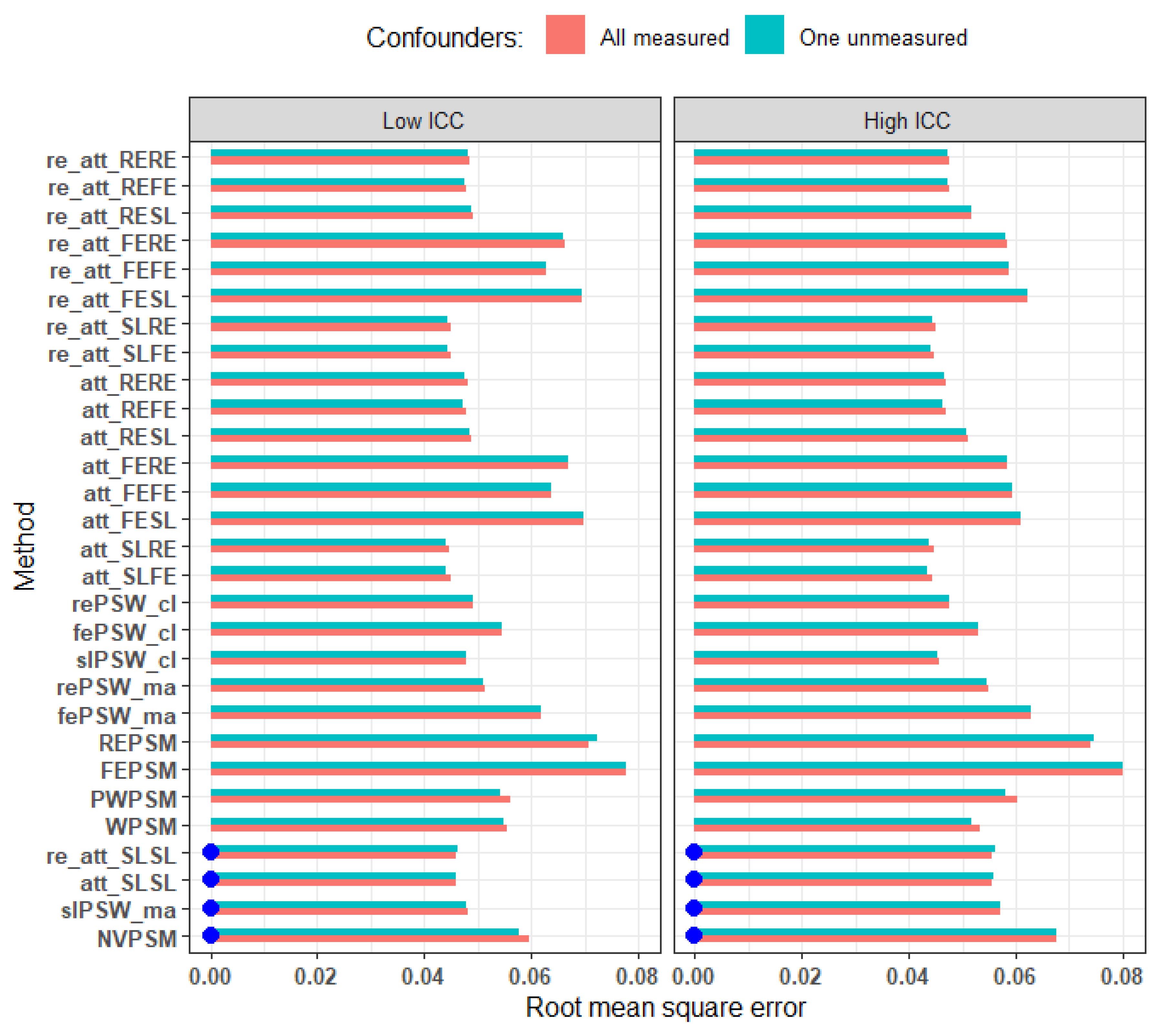
Figure 9.
Sensitivity of RMSE to the omission of a cluster-level confounder. Blue dots marker cluster-unconscious methods. Small effect, parallel response surface, high ICC, average cluster size of 100 and imbalance level of 96%. Relative deviation from equal to 1.46.
Figure 9.
Sensitivity of RMSE to the omission of a cluster-level confounder. Blue dots marker cluster-unconscious methods. Small effect, parallel response surface, high ICC, average cluster size of 100 and imbalance level of 96%. Relative deviation from equal to 1.46.
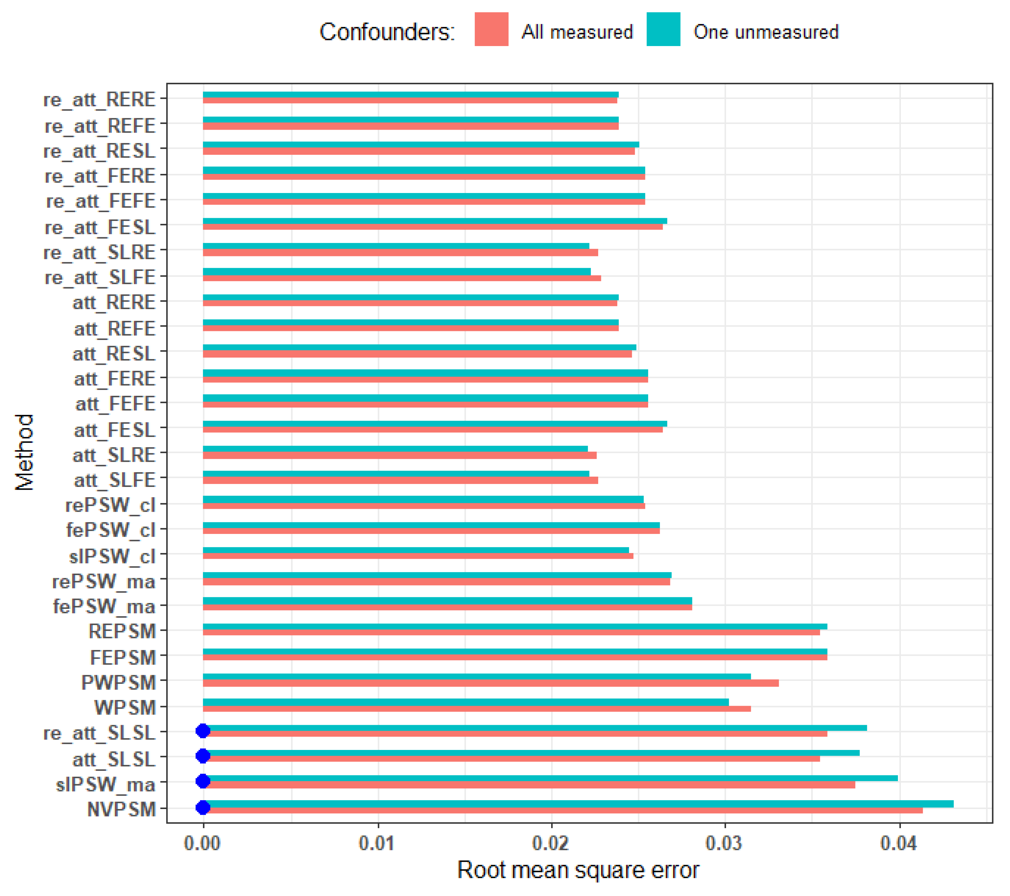
Figure 10.
Ability of the estimator to capture the actual direction of the true effect (all confounders measured, parallel response surface, perfectly balanced cluster size of 25). Blue dots mark cluster-unconscious methods.
Figure 10.
Ability of the estimator to capture the actual direction of the true effect (all confounders measured, parallel response surface, perfectly balanced cluster size of 25). Blue dots mark cluster-unconscious methods.
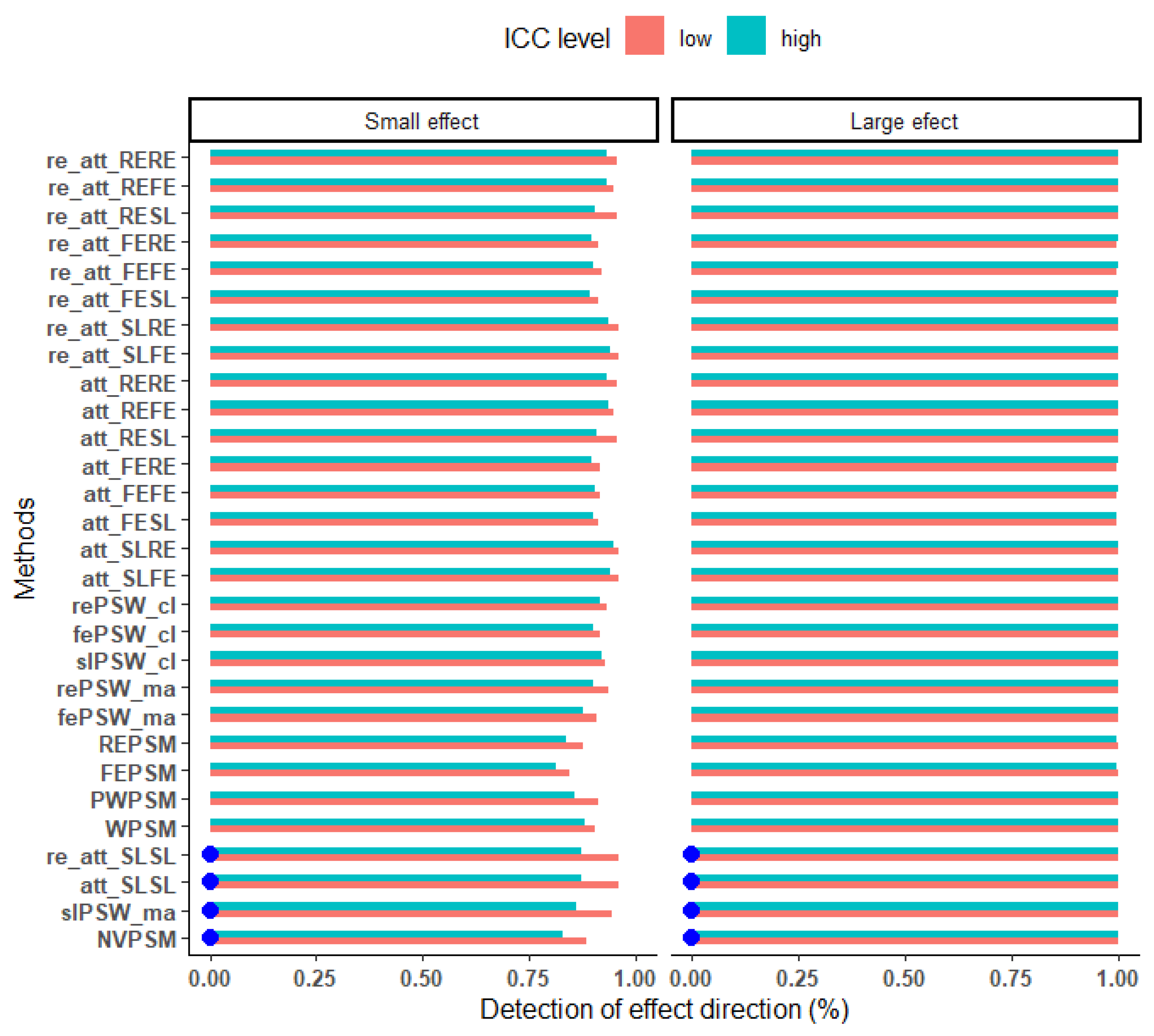
Figure 11.
Relative bias under parallel and non-parallel response surfaces. (low ICC, perfectly balanced cluster size, cluster size of 25). Blue dots mark cluster-unconscious methods.
Figure 11.
Relative bias under parallel and non-parallel response surfaces. (low ICC, perfectly balanced cluster size, cluster size of 25). Blue dots mark cluster-unconscious methods.
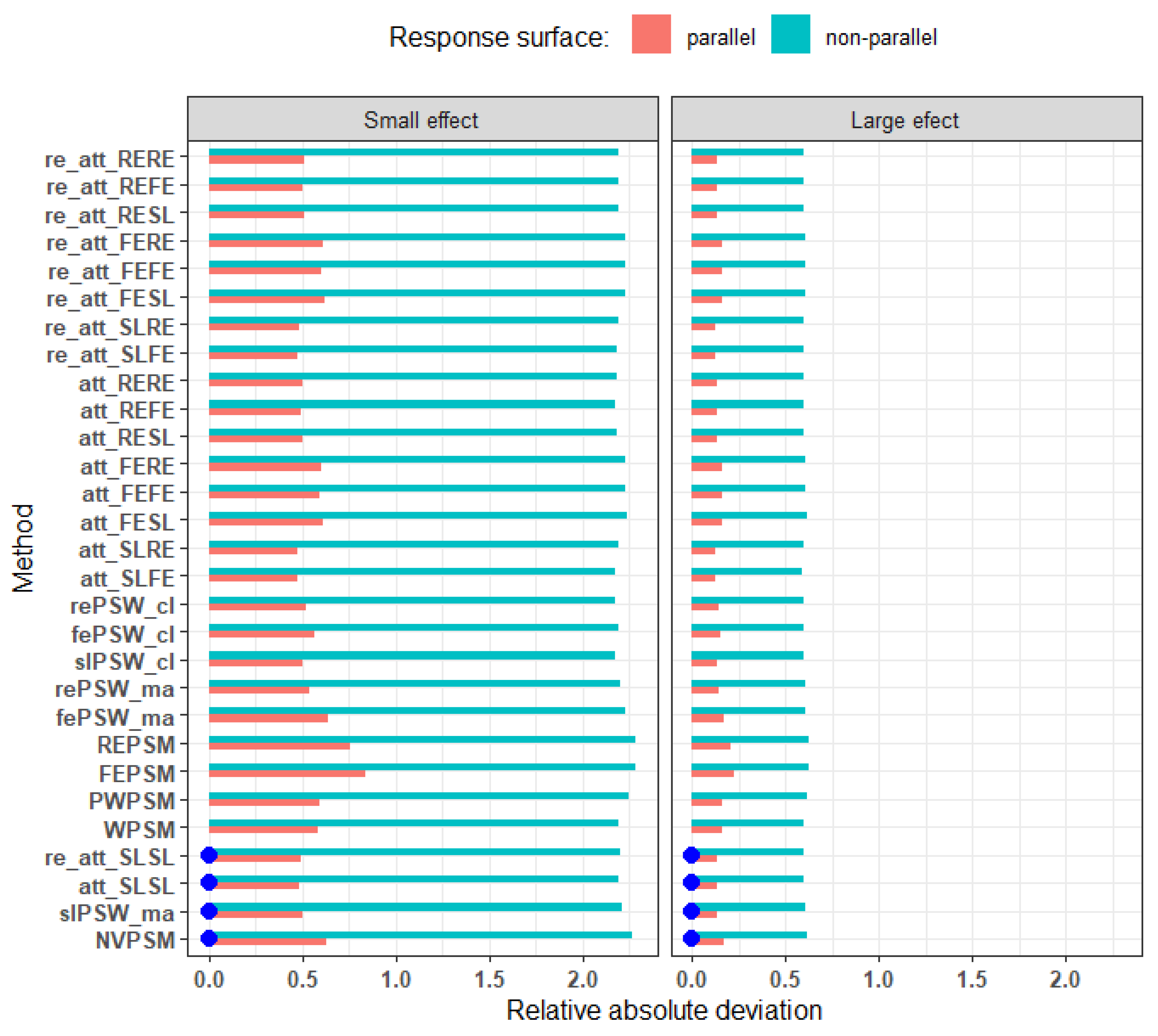
Table 1.
Investigated candidate methods to estimate ATT.
| Methods | Description | C_U | C_A |
|---|---|---|---|
| 1: PSMPM | PSM with Single-level model with matching on pooled data [21] | x | |
| 2: WPSM | PSM with Single-level model and matching purely withing cluster matching [21] | x | |
| 3: PWPSM | PSM with Single-level model and matching preferentially within cluster matching [21] | x | |
| 4: FEPSM | PSM with Fixed effect model and matching on pooled data [21] | x | |
| 5: REPSM | PSM with Random intercept model and matching on pooled data [21] | x | |
| 6: PSWSLma | PSW with weights from Single-level model, on pooled data [9] | x | |
| 7: PSWFEma | PSW with weights from Fixed effect model, on pooled data [9] | x | |
| 8: PSWREma | PSW with weights from Random intercept model, on pooled data [9] | x | |
| 9: PSWSLwc | PSW with weights from Single-level model with aggregated within clustered effect [9] | x | |
| 10: PSWFEwc | PSW with weights from Fixed effect model with aggregated within clustered effect [9] | x | |
| 11: PSWREwc | PSW with weights from Random intercept model with aggregated within clustered effect [9] | x | |
| 12: SL-SL-PSW | Double robust PSW: Single-level-based PS - Single-level-based PO [9] | x | |
| 13: SL-FE-PSW | Double robust PSW: Single-level-based PS - Fixed-effect model-based PO [9] | x | |
| 14: SL-RE-PSW | Double robust PSW: Single-level-based PS - Random effect model-based PO [9] | x | |
| 15: FE-SL-PSW | Double robust PSW: Fixed-effect model-based PS - Single-level-based PO [9] | x | |
| 16: FE-FE-PSW | Double robust PSW: Fixed-effect model-based PS - Fixed-effect model-based PO [9] | x | |
| 17: FE-RE-PSW | Double robust PSW: Fixed-effect model-based PS - Random effect model-based PO [9] | x | |
| 18: RE-SL-PSW | Double robust PSW: Random effect model-based PS - Single-level-based PO [9] | x | |
| 19: RE-FE-PSW | Double robust PSW: Random effect model-based PS - Fixed-effect model-based PO [9] | x | |
| 20: RE-RE-PSW | Double robust PSW: Random effect model-based PS - Random effect model-based PO [9] | x |
PS: Propensity score, PSW: Propensity score weighting, PSM: Propensity score matching, PO: Potential outcome; C_U: Cluster-unconscious, C_A: Cluster-aware.
Table 4.
Top two methods to estimate small size causal effects under parallel response surface.
| Mean cluster size | Imbalance | Confounders | Outcome ICC | True effect | Top 2 Methods | RMSE |
|---|---|---|---|---|---|---|
| 25 | 0.96 | All measured | 0.02 | -0.075 | att_RERE | 0.05 |
| att_RESL | 0.05 | |||||
| 0.26 | -0.064 | att_RERE | 0.05 | |||
| att_REFE | 0.05 | |||||
| One unmeasured cluster-level covariate | 0.02 | -0.075 | re_att_SLRE | 0.05 | ||
| att_RERE | 0.05 | |||||
| 0.26 | -0.064 | att_SLRE | 0.05 | |||
| att_SLFE | 0.05 | |||||
| 0.50 | All measured | 0.02 | -0.074 | att_SLRE | 0.05 | |
| re_att_SLRE | 0.05 | |||||
| 0.27 | -0.065 | att_SLRE | 0.04 | |||
| att_SLFE | 0.04 | |||||
| One unmeasured cluster-level covariate | 0.02 | -0.074 | att_SLRE | 0.05 | ||
| re_att_SLRE | 0.05 | |||||
| 0.27 | -0.065 | att_SLRE | 0.04 | |||
| att_SLFE | 0.04 | |||||
| 0.00 | All measured | 0.03 | -0.075 | att_SLRE | 0.04 | |
| att_SLFE | 0.04 | |||||
| 0.28 | -0.065 | att_SLFE | 0.04 | |||
| att_SLRE | 0.04 | |||||
| One unmeasured cluster-level covariate | 0.03 | -0.075 | att_SLFE | 0.04 | ||
| att_SLRE | 0.04 | |||||
| 0.28 | -0.065 | att_SLFE | 0.04 | |||
| att_SLRE | 0.04 | |||||
| 100 | 0.96 | All measured | 0.03 | -0.075 | att_SLRE | 0.02 |
| re_att_SLRE | 0.02 | |||||
| 0.27 | -0.066 | att_SLRE | 0.02 | |||
| att_SLFE | 0.02 | |||||
| One unmeasured cluster-level covariate | 0.03 | -0.075 | att_SLRE | 0.02 | ||
| re_att_SLRE | 0.02 | |||||
| 0.27 | -0.066 | att_SLRE | 0.02 | |||
| re_att_SLRE | 0.02 | |||||
| 0.49 | All measured | 0.04 | -0.073 | att_SLRE | 0.02 | |
| att_SLFE | 0.02 | |||||
| 0.28 | -0.064 | att_SLRE | 0.02 | |||
| att_SLFE | 0.02 | |||||
| One unmeasured cluster-level covariate | 0.04 | -0.073 | att_SLFE | 0.02 | ||
| att_SLRE | 0.02 | |||||
| 0.28 | -0.064 | att_SLRE | 0.02 | |||
| att_SLFE | 0.02 | |||||
| 0.00 | All measured | 0.04 | -0.075 | att_SLRE | 0.02 | |
| re_att_SLRE | 0.02 | |||||
| 0.28 | -0.065 | att_SLFE | 0.02 | |||
| att_SLRE | 0.02 | |||||
| One unmeasured cluster-level covariate | 0.04 | -0.075 | att_SLRE | 0.02 | ||
| re_att_SLRE | 0.02 | |||||
| 0.28 | -0.065 | att_SLFE | 0.02 | |||
| att_SLRE | 0.02 |
re_ prefix designate double robust methods that allow for interaction between individual-level covariates and exposure.
Disclaimer/Publisher’s Note: The statements, opinions and data contained in all publications are solely those of the individual author(s) and contributor(s) and not of MDPI and/or the editor(s). MDPI and/or the editor(s) disclaim responsibility for any injury to people or property resulting from any ideas, methods, instructions or products referred to in the content. |
© 2025 by the authors. Licensee MDPI, Basel, Switzerland. This article is an open access article distributed under the terms and conditions of the Creative Commons Attribution (CC BY) license (http://creativecommons.org/licenses/by/4.0/).
Copyright: This open access article is published under a Creative Commons CC BY 4.0 license, which permit the free download, distribution, and reuse, provided that the author and preprint are cited in any reuse.


