
Submitted:
27 November 2024
Posted:
28 November 2024
You are already at the latest version
Abstract
When the effect of a treatment variable on an outcome variable differs between two groups, an interaction effect is present. Since this is one of the most common statistical analyses, Stata offers a wide variety of methods to investigate such effects. The present study outlines how these different analyses can be performed in Stata and provides a comprehensive simulation study to determine which method has the best statistical properties. To this end, both the nominal alpha error rate and statistical power are assessed for continuous and binary dependent variables. For a deeper analysis, not only are the sample sizes varied, but other potential challenges are also considered, such as heteroscedasticity for the continuous outcome and imbalanced binary outcome variables. The results indicate that some methods deviate significantly from the nominal alpha limit, leading to incorrect conclusions on average. For the continuous outcome variable, the OLS regression approach with robust (HC3) standard errors and an interaction term yields the best results. For the binary outcome, we recommend the logit model with robust standard errors or the linear probability model with robust (HC3) standard errors.
Keywords:
interaction effect
; moderation effect
; nonparametric methods
; simulation study
; Stata
1. Introduction
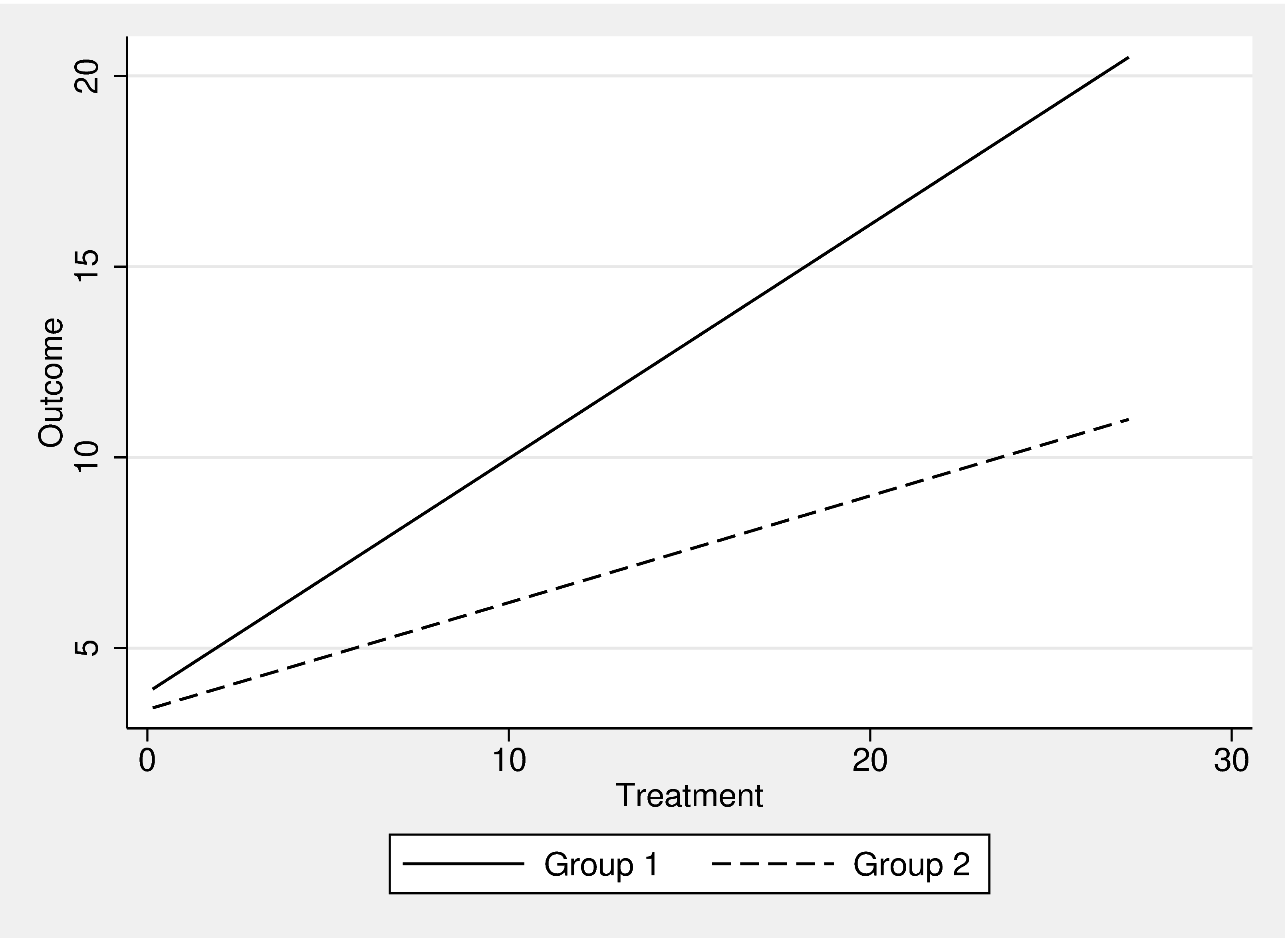
Testing for heterogeneous effects is one of the most popular and widespread applications of statistics in empirical research. Many theories predict that the effect of a treatment is not uniform but can differ between groups. For example, one might suppose that the dosage of a new antihypertensive drug works differently in men and women, and that different dosages might be required to achieve the same effect for both genders. These heterogeneous effects can have significant consequences for both empirical research and practical interventions. In regression analysis frameworks, these tests are usually referred to as interactions (sometimes also called moderation). The key idea is that the main effect of a treatment interacts with a subgroup of the sample. In Figure 1, such a process is visualized. The effect that the treatment exerts on the outcome is stronger in group 1 than in group 2, as shown by the differing slopes of the lines. While this concept is theoretically easy to grasp, there exists a large variety of potential empirical approaches to investigate such heterogeneous effects. In this paper, we introduce a wide range of potential solutions in Stata. We will investigate both continuous and binary outcome variables with a continuous treatment variable and binary groups.
To assess the statistical quality and validity of various empirical approaches, we examine two important aspects: alpha error and statistical power. The alpha error (also known as Type I error) is the probability of incorrectly rejecting the null hypothesis. Typically, the null hypothesis is formulated conservatively (assuming that the effect of the treatment is identical across all groups), while the alternative hypothesis is more liberal, suggesting that the treatment effect is heterogeneous. If the null hypothesis is incorrectly rejected, it means that one believes an effect exists when, in fact, it does not. The alpha error level is set a priori by the researcher, often at 5%. This means that, even if there is no true effect, the probability of incorrectly rejecting the null is set to this nominal level. A good statistical test should, on average, maintain this nominal level and produce a statistically significant result in no more than 5% of all samples when the null hypothesis is actually true. Deviations from this nominal level bias the statistical results and should be avoided.
The second key aspect of quality is statistical power. Power is the probability of detecting an effect when it is present in reality. Statistical tests with low power are generally unhelpful for drawing practical conclusions and should be avoided. In general, as long as alpha errors remain consistent, the approach with the higher power is preferable. However, alpha error and power are related; liberal tests tend to have higher power but do not maintain the nominal alpha error limit set by the researcher. It is therefore advisable to first select an approach that is close to the nominal alpha error limit and then assess its power. In the following paper, we will introduce a wide range of approaches available in Stata for detecting interaction effects and conduct a comprehensive simulation study to evaluate both alpha error and power. By doing so, we aim to provide practical recommendations on which approach offers the highest statistical quality. Note that all these approaches are concerned with statistical inference—i.e., whether one can generalize the findings from the sample to the broader population.
Note that this paper investigates the interaction effect of subgroups, meaning that each observation in the dataset belongs to exactly one group. Related questions include how to compare regression coefficients for the same individuals across different models (e.g., testing whether a logit or probit model is more appropriate) or how to handle overlapping group comparisons. While some of the methods introduced in this study may be applicable to these questions (particularly the Chow test and Stata’s suest command), they are not the primary focus of this research. Therefore, the empirical results presented here may not easily generalize to these related, yet distinct, research questions.
2. Continuous Dependent Variables
A continuous variable is a type of quantitative variable that can take on an infinite number of values within a given range. These values can be any real number and can be measured with great precision, depending on the level of measurement or the instrument used. Common examples include body weight or height, blood pressure, and precipitation per square meter in a month. Ideally, such a variable is also normally distributed, which is not required but can enhance inference. In the following examples, we make use of the NLSW dataset. We aim to test whether the effect of total labor market experience on wages differs by place of residence (South vs. non-South). Subsequently, we introduce a wide range of approaches to test this hypothesis empirically.
2.1. Pooled OLS
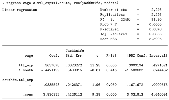
The most common approach to test for interactions is the inclusion of an interaction term in a pooled OLS model. "Pooled" means that all subgroups are combined in a single dataset or analysis. The empirical approach is as follows:
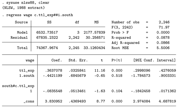
Here we utilize Stata’s notation to denote the interaction effect. The double pound sign specifies the inclusion of both the main effects of the independent variables and the interaction effect. The results show that total work experience is positively related to wages: increasing experience by one year raises wages by 36 cents per hour. The main effect of living in the South is negative, indicating that individuals in the South earn about 44 cents less than individuals in other regions, on average. Finally, we observe the interaction effect, which is negative and amounts to about 8 cents. This means that while individuals in other regions gain about 36 cents per year of work experience, this effect is only 36 - 8 = 28 cents in the South. The conclusion is that, in this particular sample, the effect of work experience on wages is smaller in the South than in other regions. However, this effect is statistically insignificant, as the reported p-value (0.104) exceeds the nominal limit of 5%, which we adopt for the rest of this paper by tradition (note that this is the sole reason for choosing this limit, and there is no deeper justification for it). If one does not want to calculate the effects manually, which can be challenging for more complex analyses with multiple groups, margins is a convenient alternative.

As you can see, the results align with the manual computations. However, to test whether these two reported results are statistically different from each other, margins is not required, as this information is already conveyed by the interaction coefficient in the main OLS output. The OLS approach is flexible and allows for the estimation of robust standard errors, which can be highly relevant if heteroscedasticity is present. This means that the variances of the outcome variable are unequal within groups. To specify the estimation with robust standard errors, add the option vce(hc1) (which is equivalent to vce(robust)) or vce(hc3), which may be even better for addressing heteroscedasticity.1
2.2. Chow Test
Sometimes, it is recommended to utilize the Chow test instead of using a pooled model. While the pooled approach is convenient, one downside is that residual group variances are not explicitly modeled. An alternative approach is to estimate separate regression models for each subgroup and then use a Wald test to compare coefficients across models. The handling in Stata is as follows.
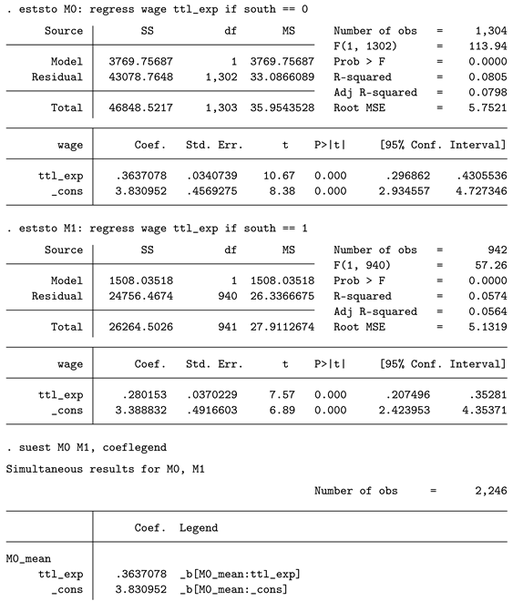
First, separate OLS regressions are estimated for each group, and the results are stored. Next, suest is used to combine these stored results. The option coeflegend is convenient, as it helps us find the correct name for the coefficients of interest. As you can already see from the regression output, the point estimates are exactly the same as those from margins in the pooled model. Finally, we conduct a Wald test to check whether the coefficients are statistically different from each other. Interestingly, in this example, the p-value (0.049) is rather different from the pooled one (0.104). Since we have set the nominal alpha level to 5%, we would conclude that experience works differently in the South than in other regions, based on the Chow test. This finding underscores that the results from different approaches do not necessarily lead to the same conclusions!
2.3. Structural Equation Modelling (SEM)
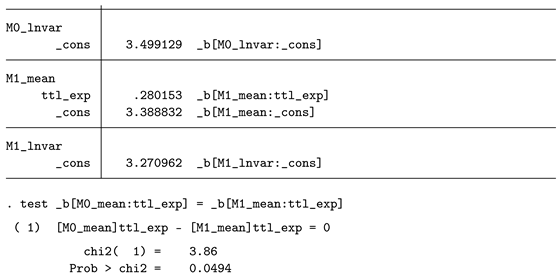
Especially in psychology, SEM is one of the most popular approaches to build models and test complex hypotheses. While the general idea is similar to conducting a regression analysis, SEM is more powerful as it enables researchers to include measurement models in their analysis and estimate large models with many dependent variables in a single step. Since all variables in our dataset are manifest and not latent, this model is typically described as a path model. We can use SEM for this kind of analysis by utilizing the group option. By doing so, the model is estimated separately for each group, and arbitrary constraints can be imposed. In this case, we do not impose any constraints but simply test empirically whether the coefficients differ after estimation. The handling is as follows:
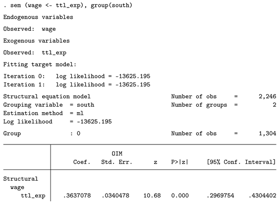
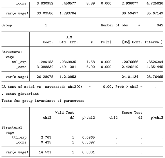
First, the main model is estimated separately for both groups. Note that SEM uses a maximum-likelihood approach, so point estimates might differ from those obtained using the OLS approach. After this step, estat ginvariant tests for group invariance and performs a Wald test. The p-value for the coefficient of interest is 0.0965. Keep in mind that the SEM approach with robust standard errors is numerically equivalent to the Chow test.
2.4. Nonparametric Approaches
The methods discussed so far are usually described as parametric approaches since they rely on certain assumptions, such as the normal distribution of sampling distributions. Nonparametric approaches, on the other hand, largely abandon such assumptions. They typically rely on resampling, reshuffling, or randomness to generate many new samples that are treated as if one had collected a completely new sample from the population. In contrast to the other methods, where only a single sample is available, this approach directly generates a sampling distribution for the statistics of interest. For completeness, this section lists three common nonparametric methods in Stata. Keep in mind that all these approaches rely only on the point estimate of interest, and no inference is required. If the program allows it, skipping the computation of standard errors or related statistics can speed up runtimes. For a general introduction to nonparametric methods in Stata, refer to [1].
2.4.1. Bootstrapping
Bootstrapping involves repeated sampling with replacement from the original data to create new samples. When this step is repeated many times (e.g., 500 times or more), one can compute the statistic of interest for each sample to generate a bootstrap distribution. While this approach can be computationally intensive, it is conceptually simple and works for any statistic of interest. In our case, we can apply the bootstrap method as a nonparametric way to determine the p-value of the interaction term. Specifically, the pooled regression is estimated for all bootstrap samples, and the standard deviation of the resulting bootstrap distribution serves as the standard error, which is then used to compute the p-value. Performing this in Stata is simple.
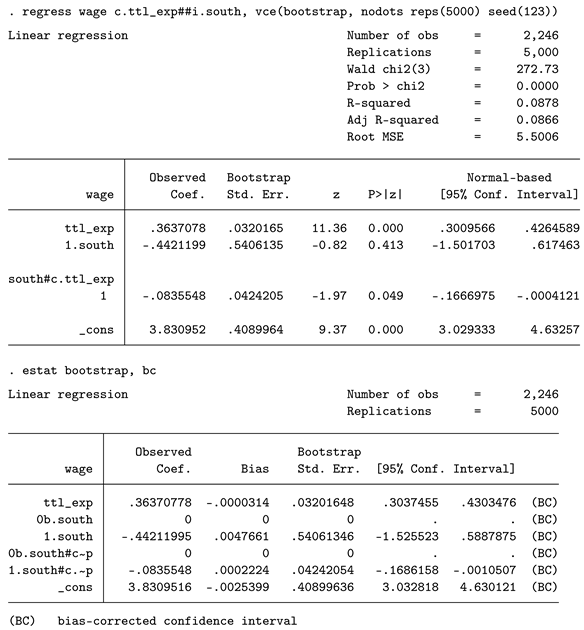
Bootstrapping and other nonparametric approaches are already strongly integrated into Stata, so using them is simple. We specify the pooled OLS model as before but instruct Stata to estimate bootstrapped standard errors using the vce option. We want 5,000 resamples and set a seed to ensure that our results are reproducible. The postestimation command estat bootstrap also provides the bootstrap bias and advanced bootstrap confidence intervals. The bootstrap p-value is 0.049, which is much lower than the regular p-value from the OLS approach. The bootstrap bias of the coefficient is very small (0.0002224). As a rule of thumb, the bootstrap bias should be at most 25% of the bootstrap standard error. If this rule is violated, the number of resamples should be increased, or an alternative approach should be considered. Regarding the number of resamples, more is always better. While 500 might be sufficient for a quick inspection of the outcome, some papers recommend 15,000 resamples for more precise results. More resamples are always better, but keep in mind that computational times can be much longer, as the regression estimation must be carried out for each resample. If time is a critical factor, abandoning regress can be helpful. One alternative is to compute the interaction effect manually and use the user-written program asreg, which is much faster.2 Note that this requires writing your own helper program. An alternative to bootstrapping is the wild cluster bootstrap approach implemented in boottest, which is usually substantially faster than regular bootstrapping [2].
2.4.2. Jackknife
The jackknife approach is similar to bootstrapping but does not rely on random draws from the sample. Instead, it follows a systematic approach by always leaving one observation out. This means that the number of required models to estimate is always as large as the pooled sample size. By doing this, a large set of jackknife resamples is created, which is then processed similarly to the bootstrap approach to generate p-values and confidence intervals. The usage is analogous.
Note that this approach does not require the user to specify a random seed or the number of resamples as this is not necessary. The generated p-value (0.050) is similar to the bootstrap p-value.
2.4.3. Permutation Tests
The logic behind the permutation test is to randomly assign group membership and observe how this affects the outcome. By doing so, the permutation test analyzes how strong the results would be, on average, if the grouping were completely random and no longer associated with the outcome. This requires specifying how many random assignments should be tested. The approach generates a p-value, which is simply the ratio of random permutations where the outcome statistic is at least as large as the observed one, divided by the total number of permutations. Note that this approach is usually less flexible, as it only works with binary groups. It works with regress but requires a short helper program, as it cannot directly access the saved coefficient from regress. Therefore, we write a program where the coefficient of interest is written to a scalar, and this scalar is then returned to permute. It works as follows:
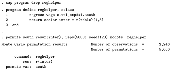
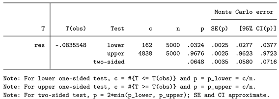
The first line ensures that any earlier versions of the helper program are removed from memory. Then, we define the program as r-class and name it reghelper. It simply computes the pooled model and returns the statistic of interest from the saved matrix. The value we want to return is the point estimate for the interaction coefficient. To locate the desired value for your own models, try matrix list r(table). If this is a different statistic, such as R-squared, use return list or ereturn list. After defining this program, you can test it. Then it must be fed into permute. The results show that the two-sided p-value is 0.0648. Again, the computation might be faster when using asreg instead of regress.
2.5. Overview
Without claiming to be exhaustive, we have outlined a wide range of options to investigate interaction effects using Stata. The main results are briefly summarized in the Table 1.
All methods will produce a p-value that can be used for inference. However, p-values are somewhat problematic, and their usage is no longer strongly encouraged. A better alternative to judge the effect size is confidence intervals, although these are only available for some of the proposed methods. If heteroscedasticity is present, some approaches allow for the computation of robust standard errors. is potentially the most robust option but is only available for the pooled OLS model. Missing data, a common problem in empirical research, can be handled most conveniently using multiple imputation with chained equations (MICE). The pooled OLS approach can be easily estimated with imputed data. While all other approaches can also work with imputed data, this always requires custom programs. Additionally, keep in mind that for many approaches, the statistical validity of these custom methods is not firmly established. To combine bootstrapping with multiple imputation, refer to [3]. Another alternative is full-information maximum likelihood with SEM using the option method(mlmv). However, note that this only works for missing values in the treatment or dependent variable, but not in the group variable. Finally, runtime can be an important consideration for large datasets or repeated estimations. While most approaches are relatively fast, nonparametric methods take much more time, as the same command needs to be estimated multiple times.
3. Binary Dependent Variables
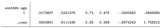
In the real world, many variables are binary by nature and can only take the values 0 or 1. The classical approach to analyze such variables is logit or probit regression. However, in recent years, using OLS and estimating linear probability models (LPM) for these binary variables has gained much popularity. Another option is to rescale logits or odds ratios to average marginal effects (AMEs). Note that for all of the following analyses, the research question is adapted, as we now need a binary outcome variable. Specifically, we ask: Does the effect that age exerts on never having been married differ between individuals living in the south or not?
3.1. Logit and Probit Regression
Logit and probit regressions are similar in that their main function is to model binary dependent variables. The main difference between the two models lies in their link function. In logit regression, the link function is the logistic function, whereas in probit regression, it is the cumulative distribution function of the standard normal distribution. While this might seem to be a rather drastic difference, both types of regressions are widely used, and their performance is generally considered to be similar. The primary difference is in the interpretation of the coefficients. In logit regression, the coefficients are either reported as logits (log odds) or odds ratios, while probit regression assumes the existence of a latent, continuous variable that determines the outcome of the binary manifest variable. The interpretation of probit coefficients is then expressed in terms of z-scores on this assumed continuous variable.
In our case, the interpretation of the coefficients is of less relevance, as we are mainly interested in p-values, which should be very similar across the two models. Below is the handling of both models.
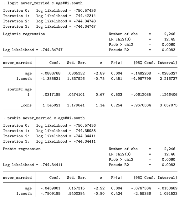
In general, interpreting logits/odds ratios or z-scores of these binary outcome models is rather unintuitive. A common suggestion is to interpret only the sign of the coefficients and nothing more. However, as you can see, while the coefficients differ considerably between the two models, the p-values are highly similar. As a result, there appears to be no statistically significant interaction effect present.
3.2. Average Marginal Effects (AMEs)
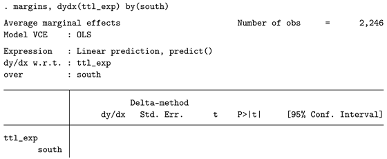
To address these potential downsides of the logit and probit models, Average Marginal Effects (AMEs) have been proposed as a solution, and they have become highly popular in recent years [4]. AMEs facilitate a more intuitive interpretation, as they express changes in probabilities. While AMEs cannot be computed directly for interaction terms, one can compute average marginal effects for both groups of interest and then compare them. Below, we demonstrate the handling of AMEs based on the logit model (though the approach also works with probit, with only marginal differences).
After estimating the logit model, we use margins to compute the AMEs. The option dydx() specifies the variable those effect we are interested in, in our case it is age. With by() we specify that this effect should be computed separately for individuals from the south and other regions. The results are shown below. The effect is -.0048832 in the south and -.0086246 in other regions. This means that when age increases by one year in the south, the probability to have never been married decreases by about 0.488 percentage points. Apparently, the effect is weaker in the south than in other regions. But is this difference statistically significant? To check this, the option pwcompare() can be used. It not only computes the difference between the two AMEs but also provides a p-value (0.389). Therefore, no statistically significant difference can be assumed based on these results.
For completeness, it should be made clear that there is also a second approach / syntax that could be used. What margins does using the by(groupvar) syntax as shown above is to factually split the sample and compute the AME for each subgroup separately. One can replicate this result by running two separate models (similar to the Chow test). An alternative is to use this command: margins south, dydx(age). What happens internally is that Stata computes a "what if" scenario. Regardless of the factual group membership, Stata first plugs in value 0 for group membership for each observation and computes the AME and then plugs in 1 and computes the AME again. The result then shows, what would the AME be if every observation is treated as a counterfactual. We believe that for the current demonstration and research question, this is not ideal. The following simulation results might differ if using the different syntax. Users should be aware of this difference and decide what fits their own needs best.
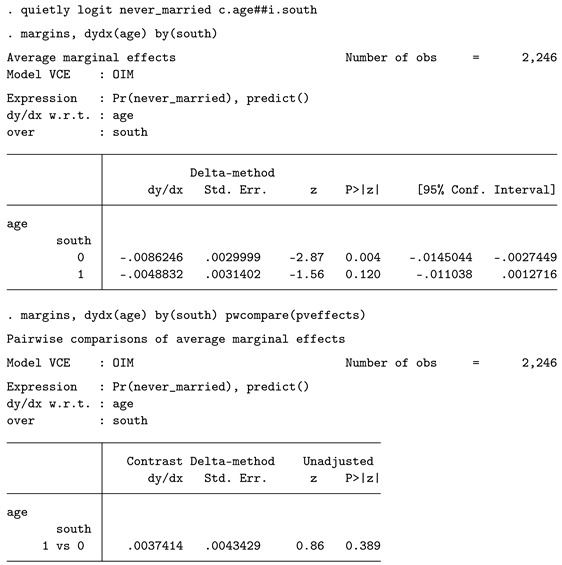
3.3. Linear Probability Model (LPM)
While it was shunned a few years ago, simply estimating an OLS regression model with a binary dependent variable has gained much popularity. Although some aspects of the OLS model are clearly violated with this approach, the general success, flexibility, and ease of interpretation have supported the usage of the LPM. The main benefit is that no transformations need to be applied, and the reported OLS regression coefficients can be directly interpreted as changes in probabilities.
For example, for individuals from regions other than the South, the effect of being one year older is -0.0083769, or -0.84 percentage points. The interaction effect is statistically not significant. Especially in these LPMs, using robust standard errors appears to be highly relevant, as the assumption of homoscedasticity is always violated.
3.4. Chow Test
Estimating separate models works for logit, probit, and regress. The application of the test is identical to that for continuous dependent variables; hence, no extra example is provided. As it turns out, the logit regression with robust standard errors is equivalent to the (logit) Chow test and probit regression with robust standard errors is equivalent to the (probit) Chow test.
3.5. Overview
A brief summary of the five methods is shown (Table 2.). Fortunately, almost all methods not only produce p-values but also provide confidence intervals for deeper insight. Most methods work with imputed data (although AMEs require a user-written ado for this purpose).3 Most methods support some form of robust standard errors, which are particularly relevant in the LPM. The runtimes are somewhat similar, with the AME and Chow approaches taking longer.

Table 2.
Overview of all methods for continuous outcome variables.
| Logit | Probit | AME | LPM | Chow | |
|---|---|---|---|---|---|
| P-value | Yes | Yes | Yes | Yes | Yes |
| SE/CI | Yes | Yes | Yes | Yes | |
| Robustness | |||||
| Missing data | MICE | MICE | (MICE) | MICE | |
| Runtimea | 3.2 | 2.9 | 9.8 | 1 | 6.6 |
a Computed for a sample size of 1,000. LPM normed to be 1 (100%). b The robust logit results are numerically equivalent to the logit Chow test. c The robust probit results are numerically equivalent to the probit Chow test.
4. Simulation Study
To test how the various methods for detecting interaction effects perform, simulation studies can be used. In a simulation study, custom datasets are generated based on random data with known distributions and parameters. By utilizing the various methods, one can test which method is closest to the target limit. Since many datasets are simulated, inference is possible. This approach has multiple advantages: one can design a dataset with very specific properties and systematically vary various parameters (such as the sample size). Since each method is tested with the same dataset, the ceteris paribus assumption is perfectly valid, which supports a fair comparison. In the simulation study, we focus on two important aspects of statistical quality: alpha error and statistical power. Both aspects have already been introduced.
4.1. Continuous Outcome Variables
We start by defining how the outcome variable y is generated. We have one continuous explanatory variable (the "treatment") and one binary explanatory variable (group membership). In the simulation, the null hypothesis is enforced, meaning there is no interaction effect, and the effect of x on the outcome is identical for both groups. This is easy to specify. However, we also want to introduce some degree of heteroscedasticity, as this is a common problem in applied statistics, and good methods should be able to account for it. For clarity, separate equations are provided by group (A and B).
with and . For convenience, we set to 0, which means that there is no main effect of the group. is set to 1. However, since is identical in both groups, the effect is the same, and thus no interaction effect is present, which enforces the null hypothesis. The main difference between the two equations is , where and . Here, is a factor we can vary.
As increases, the heteroscedasticity becomes more pronounced in group B compared to group A. Specifically, when is greater than one, the variance of the outcome in group B exceeds that in group A, creating a scenario of heteroscedasticity. The values for are chosen as 1, 1.5, and 3, representing conditions of homoscedasticity, mild heteroscedasticity, and more severe heteroscedasticity, respectively. The sample size is set to either 60, 200, or 1,000, which leads to a 3x3 design with a total of 9 simulation conditions. For each condition, 25,000 simulations are conducted to ensure a high degree of precision. For the bootstrap and permutation tests, we specify 1,000 resamples each. If possible, all methods are also estimated using the most conservative standard error approach (i.e., for SEM and for OLS).
In terms of the statistic of interest, we analyze p-values. As described above, all methods yield a p-value; this is the statistic common to all approaches. Since the null hypothesis is true by the design of the study, we expect the p-values to be uniformly distributed. Conventionally, a p-value smaller than 0.05 is regarded as "significant". If a method is accurate and the p-values are indeed uniformly distributed, we expect that about 5% of the results will fall below this threshold. If this is not the case, the method may be either too liberal or too conservative, which would be undesirable. Hence, the dependent variable of the analysis is binary. We compute logistic regression models and report average marginal effects (predicted probabilities) to compare the different methods.
The second part of the simulation focuses on statistical power. For this phase, we modify the data-generating process. We set to a value drawn from a uniform distribution between 1 and 1.5 in group B. This means that in this second part of the simulation, a true effect is present in the second group. As a result, the methods should be able to detect this difference and produce statistically significant p-values. Everything else remains the same as in the first setup. In this second part, 15,000 simulations are conducted, as fewer replications are required to achieve the same degree of precision (which has been empirically verified).
4.2. Binary Outcome Variables
The simulation is repeated for binary outcome variables, which requires a different data generation process.
Since the outcome variable is binary, it can only take values 0 or 1. In Equation 3, represents the cumulative logistic distribution function, which has a mean of 0 and a standard deviation of . The term is drawn from a normal distribution with a mean of 0 and a standard deviation of 1. The cutoff value, , is systematically varied. When , the binary variable has a mean of 0.50 (i.e., a balanced outcome). By varying to values other than 0.50, we induce imbalance in the outcome variable. As the imbalance increases, the data structure changes, making the estimation more challenging. Specifically, the larger the imbalance between the two outcomes, the greater the required sample size to estimate effects precisely, as the "event" becomes rarer. This is especially critical when many independent variables are included in the model, as a larger sample size is needed to achieve accurate results in the presence of an imbalanced outcome.
We specify three values for : 0.50, 0.65, and 0.80.4 Larger imbalances introduce additional challenges, such as the potential overfitting of predictors, especially those that are more strongly associated with the more common outcome. Standard errors also tend to increase with greater imbalance, which can adversely affect inference. The total sample size is set to either 100, 500, or 1,000. These sample sizes are chosen to account for the challenges posed by imbalanced data. As there is no true heteroscedasticity in logistic regression (this is "baked in" by the link function), there is no need to account for heteroscedasticity in the data generation process. For binary outcome variables, the most critical factors to model are the sample size and the imbalance between the two outcomes.
In total, 9 simulation conditions are tested. The data generation process is identical for both groups, so the null hypothesis holds true by design. We conduct 25,000 simulations per condition to evaluate the alpha error. All methods are estimated using both normal and robust standard errors (for the Linear Probability Model (LPM), this means ). Since the Chow test is applicable to all approaches except for AMEs, it is included in the testing. Note that nonparametric approaches are not tested for the binary outcome variable. This is because there are already many parametric approaches available for testing, and binary outcome models take longer to compute than continuous outcome models, making resampling methods less efficient for this context.
For the power simulations, the data generation process is adapted as follows:
In group B, we introduce a true effect by adding the term to differentiate the two groups. The value of is drawn from a uniform distribution between 1 and 2. For the power simulation, 15,000 replications are conducted per scenario.
5. Simulation Results
5.1. Continuous Outcome Simulation
5.1.1. Alpha Error
We begin by reporting the results for the alpha error, grouped by sample size. For ease of interpretation, we provide figures with 95% confidence intervals. Numerical results can be found in the appendix (Tables 3 and 4).
For the small sample size of 60 (Figure 2), when no group heteroscedasticity is present, the regular OLS approach and the permutation approach are closest to the target value of 0.05. The Chow test and SEM approach, however, show the largest deviations, as both methods are much too liberal. When heteroscedasticity is introduced, the results remain similar, but the OLS approach with regular standard errors becomes too liberal as heteroscedasticity increases. To summarize, in small samples, the OLS and permutation approaches appear to be the most robust in terms of controlling alpha error. We now turn to the results for the intermediate sample size of 200 (Figure 3).
In this case, the OLS approach with robust () standard errors is consistently close to the target limit. The jackknife method also performs well but is computationally more intensive. Some methods, once again, are too liberal. We conclude the alpha error analysis with the large sample size of 1,000 (Figure 4).
For the large sample size, OLS with robust standard errors continues to be a prudent choice. The permutation approach and the jackknife also perform well. Interestingly, even with a large sample, the SEM approach deviates from the target as heteroscedasticity increases.
5.1.2. Statistical Power
It is important to note that more power does not always equate to better performance. Methods that are too liberal and produce statistically significant results more frequently typically show higher power, but this power comes at the cost of an incorrect alpha level. To ensure a fair comparison, we only compare methods that achieve similar alpha error rates. The results for the small sample simulation are shown in Figure 5.
Since only the OLS approach and the permutation test exhibit acceptable nominal alpha levels, these two methods are compared. The statistical power is slightly larger for OLS than for the permutation approach. The results for the intermediate sample size are shown in Figure 6.
For this sample size, the best results in terms of alpha error were obtained with OLS with robust standard errors and the jackknife. In terms of power, the two approaches are highly similar. Finally, the results for the large sample size are shown in Figure 7.
With this large sample size, the power results are nearly identical for all methods.
5.1.3. Summary
The previous analyses focused on alpha and power individually, but to draw final conclusions, it is important to consider both. Which methods approach the nominal alpha value while maintaining good power? To answer this, we generated scatterplots of alpha vs. power by sample size. The results for gamma are merged, as presenting them separately would require additional space. The findings are displayed in Figure 8, which makes it easier to identify the best approaches. For example, when the sample size is small, both OLS and the permutation approach are close to the nominal limit of 0.05. However, the statistical power of OLS is higher, suggesting that OLS should be preferred overall.
5.2. Binary Outcome Simulation
5.2.1. Alpha Error
We begin with the results for the small sample size () in Figure 9 (numerical results are shown in the appendix, Tables 5 and 6). The two methods closest to the nominal 5% alpha limit are the logit regression with robust standard errors and the linear probability model (LPM) with robust () standard errors. When the groups are strongly unbalanced, some methods show severe deviations from the target, especially when using average marginal effects (AMEs). However, for the methods that perform well, robust standard errors appear to be necessary, as deviations are also strong without them.
Next, we consider the intermediate sample size (), shown in Figure 10. As expected, all methods perform better with larger sample sizes, but logistic regression with robust standard errors and the LPM with robust standard errors remain the best performers. Probit models also produce good results.
We conclude the alpha error results with the large sample size () condition, shown in Figure 11. As with the intermediate sample size, the results remain largely the same, with logistic regression and LPM with robust standard errors continuing to outperform other methods.
5.2.2. Statistical Power
We now turn to the results for statistical power. The results for the small sample size are shown in Figure 12, for the intermediate sample size in Figure 13, and for the large sample size in Figure 14. As it becomes rather difficult to judge which method has the best power under control of the empirically reached alpha error, we directly turn to a scatterplot analysis in the following section.
5.2.3. Summary
The previous analyses focused on alpha and power individually, but to make a final assessment, it is important to consider both together. Which method controls the nominal alpha error while providing good power? To address this, we generated scatterplots of alpha vs. power by sample size. Results for the different values are merged to save space. The findings are shown in Figure 15, which makes it easier to identify the best-performing methods.
For example, when the sample size is small, we see that both the robust logit and robust LPM approaches are close to the nominal alpha limit of 0.05. However, the logit model provides more power. For the larger sample sizes, most approaches achieve good control of alpha, but power differences remain. The probit and robust logit models appear to yield the largest power.
6. Discussion
As shown by the results of the simulation study, the method chosen to detect interaction effects can significantly influence the outcomes of statistical analyses. Some methods are overly liberal in terms of alpha error, meaning they produce p-values that are consistently too small. This leads to the incorrect rejection of the null hypothesis and results in false positives, where researchers may conclude a significant effect exists when, in reality, there is none. On the other hand, overly conservative methods may fail to detect true effects, resulting in false negatives. Both types of errors can have severe consequences for research conclusions, but our study provides guidance for selecting the most appropriate method. Ideally, a method should maintain an alpha error rate close to the nominal level. If this is not achievable, researchers must weigh which type of error (type I or type II) is more problematic for their specific analysis, and choose a method accordingly. Factors such as sample size and the presence of heteroscedasticity should also be considered in making this decision.
In terms of statistical power, higher power is generally preferred, as long as it does not compromise alpha error. As demonstrated in Figure 8 and Figure 15, power and alpha error tend to be positively correlated—methods that exhibit a larger alpha error often yield greater power. While this correlation makes sense, it highlights the importance of balancing both aspects in any analysis. Researchers should be cautious when aiming for higher power, as it may come at the cost of control over type I error. It is crucial to remember that the goal of empirical research should not be to merely "hunt" for statistically significant results, but to provide robust, reliable conclusions based on sound statistical practice.
Finally, it is relevant to make the limitations of this study transparent. This paper has aimed to list and test the most common approaches for detecting interaction effects in Stata, but it does not claim to be exhaustive. There may be additional methods or approaches, including user-written commands, that have not been considered (except where mentioned as auxiliary tools). We acknowledge that nonparametric approaches, while not tested here for binary outcomes, could be used as effectively as they are for continuous dependent variables. If researchers wish to explore nonparametric methods, adapting the continuous-variable examples is straightforward.
Furthermore, the simulation study was designed to reflect a range of "realistic" scenarios that researchers might encounter in practice, but this selection of scenarios was necessarily limited. For instance, some researchers may face even smaller sample sizes than the minimum of 60 or 100 used in this study. These numbers were chosen as reasonable lower bounds to ensure robust statistical analysis. While some may argue that as few as 5 or 10 cases per group could suffice for valid statistical conclusions, we believe that a minimum of 30 cases per group is a more practical lower threshold. This is in line with common statistical conventions that recommend at least 30 observations for reliable inference [5], where the central limit theorem sets in.
The disturbance factors chosen for the simulations, such as heteroscedasticity and imbalanced binary outcomes, were intended to reflect moderate cases of imbalance. Some might suggest that even more extreme scenarios should have been tested, which is a valid point. However, due to space constraints in the paper, it was not feasible to cover all potential variations. Researchers are encouraged to repeat these simulations with different specifications that better match their specific data and research needs. This process, known as calibration, can help tailor simulations to particular research contexts and provide more precise insights.
Another limitation of the study is that it only investigated a single p-value cutoff (0.05), which is widely used in statistical inference. However, researchers often use other significance thresholds (e.g., 0.01 or 0.001). While these alternative cutoffs might yield different results, they would also require more replications due to the need for examining the extreme tails of the distribution, thus making the simulation studies more computationally intensive.
Keep in mind that this study assumes equal group sizes, which is a common assumption in many statistical models. However, real-world data often involves unequal group sizes. Investigating methods with unequal group sizes may yield different results and is an area for future research.
Finally, there is a highly relevant point that should be considered. This paper has only discussed p-values as a statistical tool to differentiate between "statistically significant" and "statistically insignificant" with an arbitrary cutoff value of 0.05. We would like to underscore that in applied research, such binary conclusions do more harm than good and should be avoided. In recent years, a shift has emerged that has rightly criticized this handling of data and statistical conclusions. Better and more nuanced methods to analyze and judge data are not only required but also already available. In this paper, we have chosen this rather traditional way of analysis because it is simpler and more practical for conducting simulations to judge whether a result is "true" and aligns with a hypothesis. Some methods, such as permutation tests or the Chow test, also only provide a p-value and nothing more, which highlights the limitations of such methods. Therefore, p-values were the only way to compare all methods in this study. We strongly urge researchers to look beyond p-values in their own analyses. While many novel approaches are available, Stata also offers several alternatives. For example, many methods provide confidence intervals or standard errors (which can be used to compute confidence intervals). Other measurements of effect sizes are also available. For example, OLS models support estat esize to compute effect sizes, which provide much more informative results than p-values alone. It is also important to note that this paper only studied statistical inference and not whether the point estimates themselves are sensible or correct.
To expand even more on this topic, even such single-statistic judgments of interaction effects might be insufficient. This is especially true for binary outcome variables, where nonlinear effects are almost always present. In such cases, using predicted values and graphs is a powerful option to understand in much more detail the dynamics of effects between groups. We provide a concrete example and compare two models: a Linear Probability Model (LPM) and a logistic regression model. In this case, inference is not the main focus, and confidence bands are not even shown to keep the figures simple. However, it becomes clear that conclusions can change, depending on the type of model specification. The results are shown in Figure 16, where the blood lead concentration (log) is the only explanatory variable.
On the left-hand side of the graph, logit and regress are compared, where lead is the only predictor in the model. It becomes clear that logit picks up some nonlinear trend, while regress does not. Whenever we see perfectly linear trends, we should be alerted, as in reality, at least subtle nonlinearities are often present. To test this empirically, we can add a higher-order term explicitly to the models.5 The results, after doing this, are shown on the right-hand side. In the logit model, the nonlinear trends are now even more pronounced, while in the regress model, these trends also appear. Apparently, the models on the right-hand side are much better for understanding what is actually going on in the data.
Therefore, keep in mind that not only the general approach is relevant, but also building a good statistical model that is properly visualized. The graphs, conveniently created with margins, provide much more insight than simple regression tables ever could 6.
7. Conclusion and Recommendation
When the effect a treatment exerts on the outcome differs by group, there are many options to investigate this using Stata. As the empirical part of this paper has demonstrated, some are better than others. When the outcome variable is continuous, an OLS regression model with an interaction term and robust () standard errors is probably the most prudent choice, unless the sample size is very small (total N smaller than 200). In such cases, relying on regular standard errors (or maybe the slightly less conservative robust standard error ) might be better to reach the nominal alpha error limit. An alternative are nonparametric approaches such as permutation tests, however, their most relevant downside are much longer computational times.
When the outcome variable is binary, many models have good statistical properties, as long as the total sample size is not very small. Logit (with robust standard errors), probit (regular and robust standard errors), and the LPM (only with robust standard errors) are all acceptable. For very small samples, the robust logit or robust LPM are potentially the most sensible choices.
Author Contributions
Felix Bittmann is a postdoctoral research fellow at the Leibniz Institute for Educational Trajectories (LIfBi) in Bamberg, Germany. Trained as a sociologist, his research interests span a range of topics within the social sciences, including the emergence of social inequality in educational systems, life satisfaction, and advanced methodological approaches to quantitative analysis.
Appendix A
Table A1.
Alpha simulation. Probability to have a p-value smaller than 0.05 for the continuous outcome variable. 95% confidence intervals in brackets.
Table A1.
Alpha simulation. Probability to have a p-value smaller than 0.05 for the continuous outcome variable. 95% confidence intervals in brackets.
| N | 60 | 60 | 60 | 200 | 200 | 200 | 1000 | 1000 | 1000 |
|---|---|---|---|---|---|---|---|---|---|
| Gamma | 1 | 1.5 | 3 | 1 | 1.5 | 3 | 1 | 1.5 | 3 |
| OLS | 0.0480 | 0.0491 | 0.0563 | 0.0548 | 0.0558 | 0.0630 | 0.0548 | 0.0551 | 0.0622 |
| [0.045,0.051] | [0.046,0.052] | [0.053,0.059] | [0.052,0.058] | [0.053,0.059] | [0.060,0.066] | [0.052,0.058] | [0.052,0.058] | [0.059,0.065] | |
| OLS/ROB | 0.0428 | 0.0424 | 0.0442 | 0.0513 | 0.0509 | 0.0515 | 0.0512 | 0.0508 | 0.0512 |
| [0.040,0.045] | [0.040,0.045] | [0.042,0.047] | [0.049,0.054] | [0.048,0.054] | [0.049,0.054] | [0.049,0.054] | [0.048,0.054] | [0.048,0.054] | |
| CHOW | 0.0754 | 0.0756 | 0.0756 | 0.0614 | 0.0619 | 0.0620 | 0.0536 | 0.0531 | 0.0536 |
| [0.072,0.079] | [0.072,0.079] | [0.072,0.079] | [0.058,0.064] | [0.059,0.065] | [0.059,0.065] | [0.051,0.056] | [0.050,0.056] | [0.051,0.056] | |
| SEM | 0.0623 | 0.0637 | 0.0705 | 0.0587 | 0.0603 | 0.0672 | 0.0553 | 0.0558 | 0.0630 |
| [0.059,0.065] | [0.061,0.067] | [0.067,0.074] | [0.056,0.062] | [0.057,0.063] | [0.064,0.070] | [0.052,0.058] | [0.053,0.059] | [0.060,0.066] | |
| SEM/ROB | 0.0754 | 0.0756 | 0.0756 | 0.0614 | 0.0619 | 0.0620 | 0.0536 | 0.0531 | 0.0536 |
| [0.072,0.079] | [0.072,0.079] | [0.072,0.079] | [0.058,0.064] | [0.059,0.065] | [0.059,0.065] | [0.051,0.056] | [0.050,0.056] | [0.051,0.056] | |
| BOOT | 0.0558 | 0.0568 | 0.0593 | 0.0585 | 0.0582 | 0.0590 | 0.0534 | 0.0530 | 0.0531 |
| [0.053,0.059] | [0.054,0.060] | [0.056,0.062] | [0.056,0.061] | [0.055,0.061] | [0.056,0.062] | [0.051,0.056] | [0.050,0.056] | [0.050,0.056] | |
| PERM | 0.0473 | 0.0476 | 0.0470 | 0.0535 | 0.0527 | 0.0526 | 0.0519 | 0.0518 | 0.0524 |
| [0.045,0.050] | [0.045,0.050] | [0.044,0.050] | [0.051,0.056] | [0.050,0.055] | [0.050,0.055] | [0.049,0.055] | [0.049,0.055] | [0.050,0.055] | |
| JACK | 0.0444 | 0.0445 | 0.0462 | 0.0519 | 0.0514 | 0.0520 | 0.0512 | 0.0510 | 0.0513 |
| [0.042,0.047] | [0.042,0.047] | [0.044,0.049] | [0.049,0.055] | [0.049,0.054] | [0.049,0.055] | [0.049,0.054] | [0.048,0.054] | [0.049,0.054] |
Table A2.
Power simulation. Probability to have a p-value smaller than 0.05 for the continuous outcome variable. 95% confidence intervals in brackets.
Table A2.
Power simulation. Probability to have a p-value smaller than 0.05 for the continuous outcome variable. 95% confidence intervals in brackets.
| N | 60 | 60 | 60 | 200 | 200 | 200 | 1000 | 1000 | 1000 |
|---|---|---|---|---|---|---|---|---|---|
| Gamma | 1 | 1.5 | 3 | 1 | 1.5 | 3 | 1 | 1.5 | 3 |
| OLS | 0.235 | 0.237 | 0.234 | 0.536 | 0.533 | 0.515 | 0.794 | 0.794 | 0.787 |
| [0.228,0.242] | [0.230,0.243] | [0.227,0.241] | [0.528,0.544] | [0.525,0.541] | [0.507,0.523] | [0.788,0.801] | [0.787,0.800] | [0.780,0.793] | |
| OLS/ROB | 0.206 | 0.203 | 0.188 | 0.521 | 0.514 | 0.476 | 0.791 | 0.788 | 0.774 |
| [0.200,0.213] | [0.197,0.210] | [0.181,0.194] | [0.513,0.529] | [0.506,0.522] | [0.468,0.484] | [0.784,0.798] | [0.782,0.795] | [0.767,0.780] | |
| CHOW | 0.281 | 0.275 | 0.258 | 0.543 | 0.537 | 0.500 | 0.793 | 0.790 | 0.776 |
| [0.274,0.288] | [0.268,0.282] | [0.251,0.265] | [0.535,0.551] | [0.529,0.545] | [0.492,0.508] | [0.786,0.799] | [0.784,0.797] | [0.769,0.783] | |
| SEM | 0.266 | 0.264 | 0.263 | 0.544 | 0.541 | 0.525 | 0.795 | 0.794 | 0.788 |
| [0.259,0.273] | [0.257,0.271] | [0.256,0.270] | [0.536,0.552] | [0.533,0.549] | [0.517,0.533] | [0.788,0.801] | [0.787,0.800] | [0.781,0.794] | |
| SEM/ROB | 0.281 | 0.275 | 0.258 | 0.543 | 0.537 | 0.500 | 0.793 | 0.790 | 0.776 |
| [0.274,0.288] | [0.268,0.282] | [0.251,0.265] | [0.535,0.551] | [0.529,0.545] | [0.492,0.508] | [0.786,0.799] | [0.784,0.797] | [0.769,0.783] | |
| BOOT | 0.246 | 0.242 | 0.230 | 0.537 | 0.529 | 0.494 | 0.793 | 0.789 | 0.776 |
| [0.239,0.253] | [0.235,0.249] | [0.223,0.237] | [0.529,0.545] | [0.521,0.537] | [0.486,0.502] | [0.786,0.799] | [0.783,0.796] | [0.769,0.782] | |
| PERM | 0.218 | 0.213 | 0.196 | 0.524 | 0.517 | 0.479 | 0.790 | 0.788 | 0.773 |
| [0.212,0.225] | [0.206,0.219] | [0.190,0.202] | [0.516,0.532] | [0.509,0.525] | [0.471,0.487] | [0.784,0.797] | [0.781,0.794] | [0.767,0.780] | |
| JACK | 0.211 | 0.208 | 0.192 | 0.522 | 0.515 | 0.477 | 0.791 | 0.789 | 0.774 |
| [0.205,0.218] | [0.202,0.214] | [0.185,0.198] | [0.514,0.530] | [0.507,0.523] | [0.469,0.485] | [0.785,0.798] | [0.782,0.795] | [0.767,0.780] |
Table A3.
Alpha simulation. Probability to have a p-value smaller than 0.05 for the binary outcome variable. 95% confidence intervals in brackets.
Table A3.
Alpha simulation. Probability to have a p-value smaller than 0.05 for the binary outcome variable. 95% confidence intervals in brackets.
| N | 100 | 100 | 100 | 500 | 500 | 500 | 1000 | 1000 | 1000 |
|---|---|---|---|---|---|---|---|---|---|
| Phi | 0.50 | 0.65 | 0.80 | 0.50 | 0.65 | 0.80 | 0.50 | 0.65 | 0.80 |
| Logit | 0.0288 | 0.0236 | 0.0117 | 0.0420 | 0.0404 | 0.0390 | 0.0445 | 0.0441 | 0.0401 |
| [0.027,0.031] | [0.022,0.025] | [0.010,0.013] | [0.040,0.045] | [0.038,0.043] | [0.037,0.041] | [0.042,0.047] | [0.042,0.047] | [0.038,0.043] | |
| Logit/Rob | 0.0475 | 0.0498 | 0.0608 | 0.0491 | 0.0464 | 0.0498 | 0.0502 | 0.0507 | 0.0498 |
| [0.045,0.050] | [0.047,0.053] | [0.058,0.064] | [0.046,0.052] | [0.044,0.049] | [0.047,0.052] | [0.048,0.053] | [0.048,0.053] | [0.047,0.053] | |
| Probit | 0.0394 | 0.0350 | 0.0210 | 0.0490 | 0.0457 | 0.0485 | 0.0497 | 0.0509 | 0.0486 |
| [0.037,0.042] | [0.033,0.037] | [0.019,0.023] | [0.046,0.052] | [0.043,0.048] | [0.046,0.051] | [0.047,0.052] | [0.048,0.054] | [0.046,0.051] | |
| Probit/Rob | 0.0666 | 0.0704 | 0.0915 | 0.0544 | 0.0508 | 0.0571 | 0.0512 | 0.0532 | 0.0536 |
| [0.063,0.070] | [0.067,0.074] | [0.088,0.095] | [0.052,0.057] | [0.048,0.053] | [0.054,0.060] | [0.048,0.054] | [0.050,0.056] | [0.051,0.056] | |
| AME | 0.0779 | 0.0846 | 0.0979 | 0.0682 | 0.0714 | 0.0798 | 0.0658 | 0.0725 | 0.0797 |
| [0.075,0.081] | [0.081,0.088] | [0.094,0.102] | [0.065,0.071] | [0.068,0.075] | [0.076,0.083] | [0.063,0.069] | [0.069,0.076] | [0.076,0.083] | |
| AME/Rob | 0.0923 | 0.0998 | 110 | 0.0763 | 0.0765 | 0.0802 | 0.0728 | 0.0774 | 0.0774 |
| [0.089,0.096] | [0.096,0.104] | [0.106,0.113] | [0.073,0.080] | [0.073,0.080] | [0.077,0.084] | [0.070,0.076] | [0.074,0.081] | [0.074,0.081] | |
| LPM | 0.00852 | 0.0188 | 0.0835 | 0.00804 | 0.0149 | 0.0742 | 0.00792 | 0.0158 | 0.0759 |
| [0.007,0.010] | [0.017,0.020] | [0.080,0.087] | [0.007,0.009] | [0.013,0.016] | [0.071,0.077] | [0.007,0.009] | [0.014,0.017] | [0.073,0.079] | |
| LPM/Rob | 0.0447 | 0.0427 | 0.0540 | 0.0480 | 0.0476 | 0.0482 | 0.0470 | 0.0501 | 0.0512 |
| [0.042,0.047] | [0.040,0.045] | [0.051,0.057] | [0.045,0.051] | [0.045,0.050] | [0.046,0.051] | [0.044,0.050] | [0.047,0.053] | [0.048,0.054] | |
| Chow/Logit | 0.0475 | 0.0498 | 0.0608 | 0.0491 | 0.0464 | 0.0498 | 0.0502 | 0.0507 | 0.0498 |
| [0.045,0.050] | [0.047,0.053] | [0.058,0.064] | [0.046,0.052] | [0.044,0.049] | [0.047,0.052] | [0.048,0.053] | [0.048,0.053] | [0.047,0.053] | |
| Chow/Probit | 0.0666 | 0.0704 | 0.0915 | 0.0544 | 0.0508 | 0.0571 | 0.0512 | 0.0532 | 0.0536 |
| [0.063,0.070] | [0.067,0.074] | [0.088,0.095] | [0.052,0.057] | [0.048,0.053] | [0.054,0.060] | [0.048,0.054] | [0.050,0.056] | [0.051,0.056] | |
| Chow/LPM | 0.0610 | 0.0618 | 0.0758 | 0.0524 | 0.0513 | 0.0528 | 0.0487 | 0.0519 | 0.0529 |
| [0.058,0.064] | [0.059,0.065] | [0.072,0.079] | [0.050,0.055] | [0.049,0.054] | [0.050,0.056] | [0.046,0.051] | [0.049,0.055] | [0.050,0.056] |
Table A4.
Power simulation. Probability to have a p-value smaller than 0.05 for the binary outcome variable. 95% confidence intervals in brackets.
Table A4.
Power simulation. Probability to have a p-value smaller than 0.05 for the binary outcome variable. 95% confidence intervals in brackets.
| N | 100 | 100 | 100 | 500 | 500 | 500 | 1000 | 1000 | 1000 |
|---|---|---|---|---|---|---|---|---|---|
| Phi | 0.5 | 0.65 | 0.8 | 0.5 | 0.65 | 0.8 | 0.5 | 0.65 | 0.8 |
| Logit | 0.116 | 0.1 | 0.046 | 0.57 | 0.551 | 0.445 | 0.719 | 0.7 | 0.625 |
| [0.111,0.121] | [0.095,0.105] | [0.043,0.049] | [0.562,0.578] | [0.543,0.559] | [0.437,0.453] | [0.711,0.726] | [0.693,0.708] | [0.617,0.633] | |
| Logit/Rob | 0.179 | 0.17 | 0.136 | 0.588 | 0.57 | 0.473 | 0.728 | 0.71 | 0.641 |
| [0.173,0.185] | [0.164,0.176] | [0.130,0.141] | [0.580,0.595] | [0.562,0.578] | [0.465,0.481] | [0.721,0.735] | [0.703,0.717] | [0.633,0.649] | |
| Probit | 0.153 | 0.14 | 0.0817 | 0.592 | 0.579 | 0.499 | 0.73 | 0.715 | 0.663 |
| [0.147,0.158] | [0.135,0.146] | [0.077,0.086] | [0.584,0.600] | [0.572,0.587] | [0.491,0.507] | [0.723,0.737] | [0.708,0.722] | [0.656,0.671] | |
| Probit/Rob | 0.229 | 0.224 | 0.199 | 0.599 | 0.586 | 0.513 | 0.732 | 0.718 | 0.666 |
| [0.222,0.236] | [0.217,0.231] | [0.192,0.205] | [0.591,0.607] | [0.579,0.594] | [0.505,0.521] | [0.725,0.740] | [0.711,0.725] | [0.659,0.674] | |
| AME | 0.206 | 0.225 | 0.279 | 0.542 | 0.577 | 0.645 | 0.701 | 0.722 | 0.755 |
| [0.200,0.213] | [0.218,0.232] | [0.272,0.286] | [0.534,0.550] | [0.569,0.585] | [0.637,0.652] | [0.694,0.709] | [0.715,0.730] | [0.748,0.762] | |
| AME/Rob | 0.234 | 0.247 | 0.294 | 0.554 | 0.586 | 0.643 | 0.711 | 0.728 | 0.754 |
| [0.227,0.241] | [0.240,0.254] | [0.286,0.301] | [0.546,0.562] | [0.578,0.594] | [0.635,0.651] | [0.703,0.718] | [0.720,0.735] | [0.747,0.761] | |
| LPM | 0.0371 | 0.0732 | 0.221 | 0.254 | 0.371 | 0.601 | 0.484 | 0.583 | 0.737 |
| [0.034,0.040] | [0.069,0.077] | [0.215,0.228] | [0.247,0.261] | [0.363,0.379] | [0.593,0.609] | [0.476,0.492] | [0.575,0.591] | [0.730,0.744] | |
| LPM/Rob | 0.123 | 0.131 | 0.175 | 0.456 | 0.499 | 0.571 | 0.653 | 0.675 | 0.713 |
| [0.117,0.128] | [0.125,0.136] | [0.169,0.181] | [0.448,0.464] | [0.491,0.507] | [0.563,0.579] | [0.646,0.661] | [0.668,0.683] | [0.706,0.720] | |
| Chow/Logit | 0.179 | 0.17 | 0.136 | 0.588 | 0.57 | 0.473 | 0.728 | 0.71 | 0.641 |
| [0.173,0.185] | [0.164,0.176] | [0.130,0.141] | [0.580,0.595] | [0.562,0.578] | [0.465,0.481] | [0.721,0.735] | [0.703,0.717] | [0.633,0.649] | |
| Chow/Probit | 0.229 | 0.224 | 0.199 | 0.599 | 0.586 | 0.513 | 0.732 | 0.718 | 0.666 |
| [0.222,0.236] | [0.217,0.231] | [0.192,0.205] | [0.591,0.607] | [0.579,0.594] | [0.505,0.521] | [0.725,0.740] | [0.711,0.725] | [0.659,0.674] | |
| Chow/LPM | 0.159 | 0.168 | 0.22 | 0.466 | 0.508 | 0.579 | 0.657 | 0.678 | 0.717 |
| [0.153,0.165] | [0.162,0.174] | [0.213,0.226] | [0.458,0.474] | [0.500,0.516] | [0.571,0.587] | [0.649,0.664] | [0.670,0.685] | [0.709,0.724] |
References
- Bittmann, F. Bootstrapping: an integrated approach with Python and Stata; Walter de Gruyter, 2021.
- Roodman, D.; Nielsen, M. .; MacKinnon, J.G.; Webb, M.D. Fast and wild: Bootstrap inference in Stata using boottest. The Stata Journal 2019, 19, 4–60. [Google Scholar] [CrossRef]
- Bittmann, F. Applied Bootstrap Analysis With Imputed Data in Stata 2024.
- Mood, C. Logistic regression: Why we cannot do what we think we can do, and what we can do about it. European sociological review 2010, 26, 67–82. [Google Scholar] [CrossRef]
- Cohen, J. A Power Primer. Psychological Bulletin 1992, 112, 155–159. [Google Scholar] [CrossRef] [PubMed]
- Bittmann, F. Stata: A really short introduction; Walter de Gruyter, 2019.
| 1 | For more information on this topic refer to https://blog.stata.com/2022/10/06/heteroskedasticity-robust-standard-errors-some-practical-considerations/
|
| 2 | |
| 3 | Use mimrgns by Daniel Klein (https://ideas.repec.org/c/boc/bocode/s457795.html) |
| 4 | Our tests have shown that when the imbalance becomes even larger, some models with small sample sizes fail to converge, yielding no results. |
| 5 | Stata helps us out with the efficient factor variable notation, such as logit outcome c.treatment##c.treatment##i.group
|
| 6 | For a tutorial on how to do this in Stata, refer to [6] |
Figure 1.
Interaction effect visualized. The effect of the treatment on the outcome differs by group.
Figure 1.
Interaction effect visualized. The effect of the treatment on the outcome differs by group.
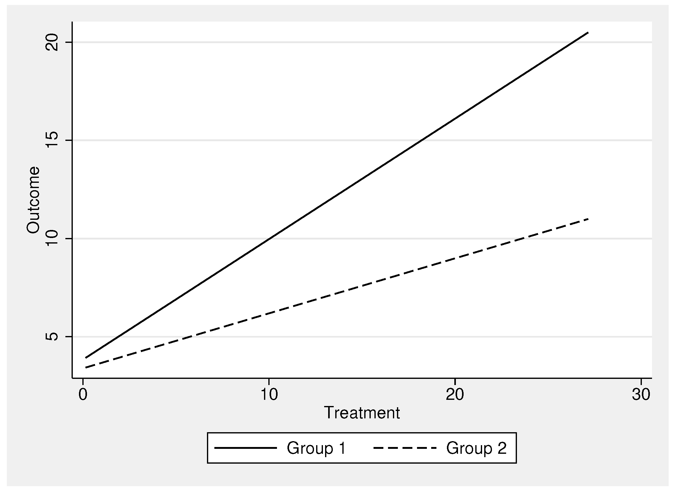
Figure 2.
Probability of obtaining a p-value smaller than 0.05 by method. Total , 25,000 simulations per condition. 95% confidence intervals included.
Figure 2.
Probability of obtaining a p-value smaller than 0.05 by method. Total , 25,000 simulations per condition. 95% confidence intervals included.
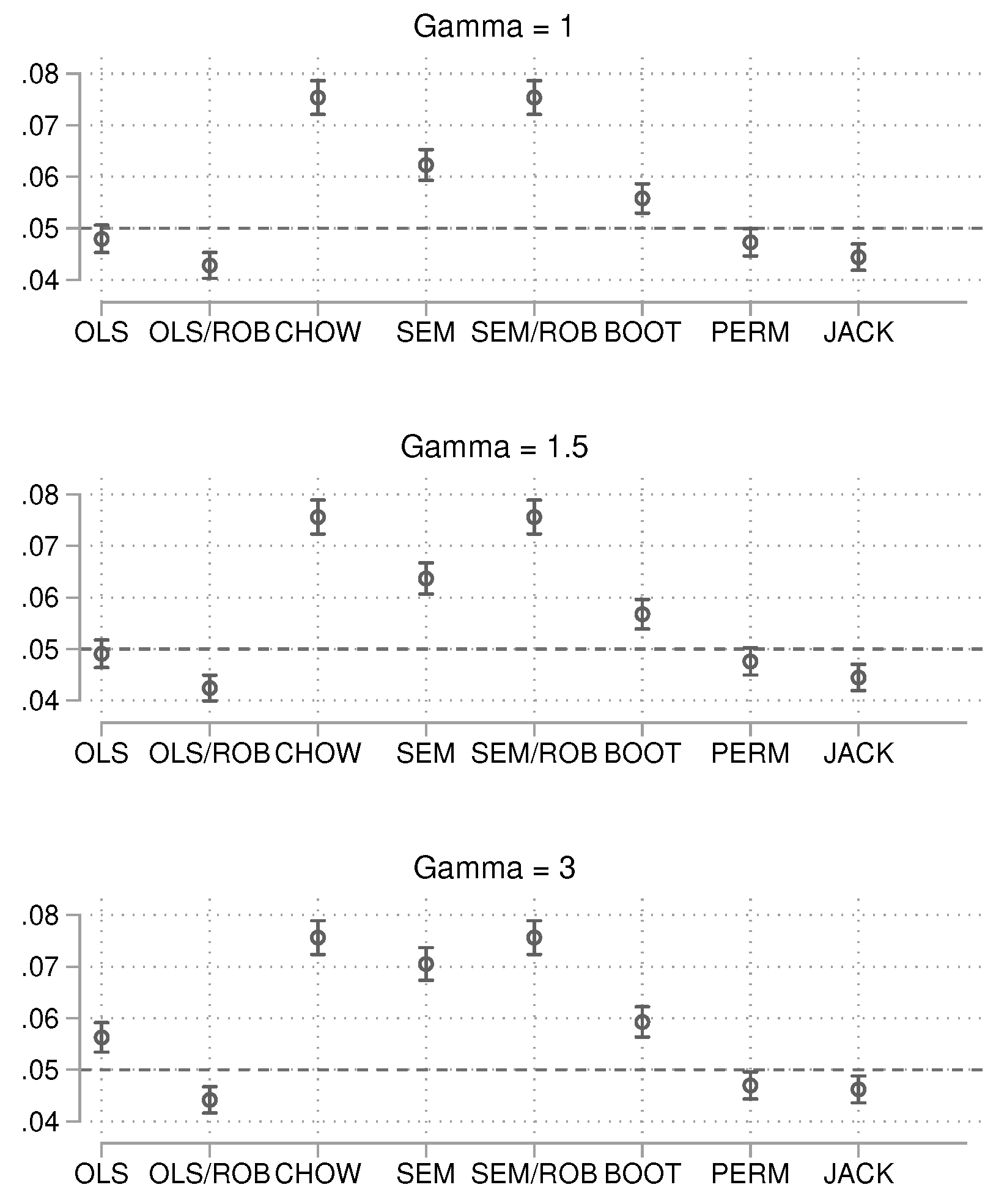
Figure 3.
Probability of obtaining a p-value smaller than 0.05 by method. Total , 25,000 simulations per condition. 95% confidence intervals included.
Figure 3.
Probability of obtaining a p-value smaller than 0.05 by method. Total , 25,000 simulations per condition. 95% confidence intervals included.
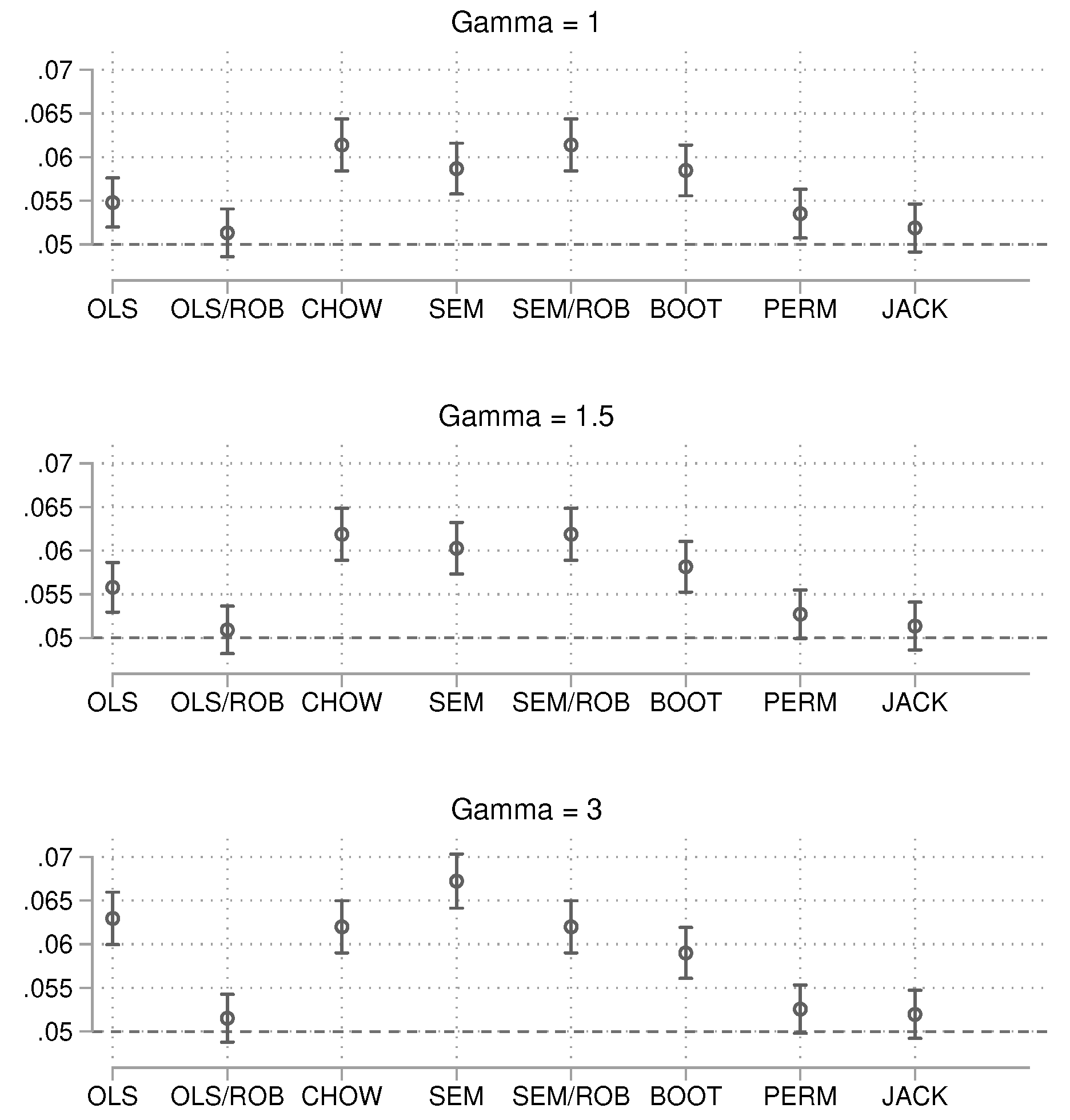
Figure 4.
Probability of obtaining a p-value smaller than 0.05 by method. Total , 25,000 simulations per condition. 95% confidence intervals included.
Figure 4.
Probability of obtaining a p-value smaller than 0.05 by method. Total , 25,000 simulations per condition. 95% confidence intervals included.
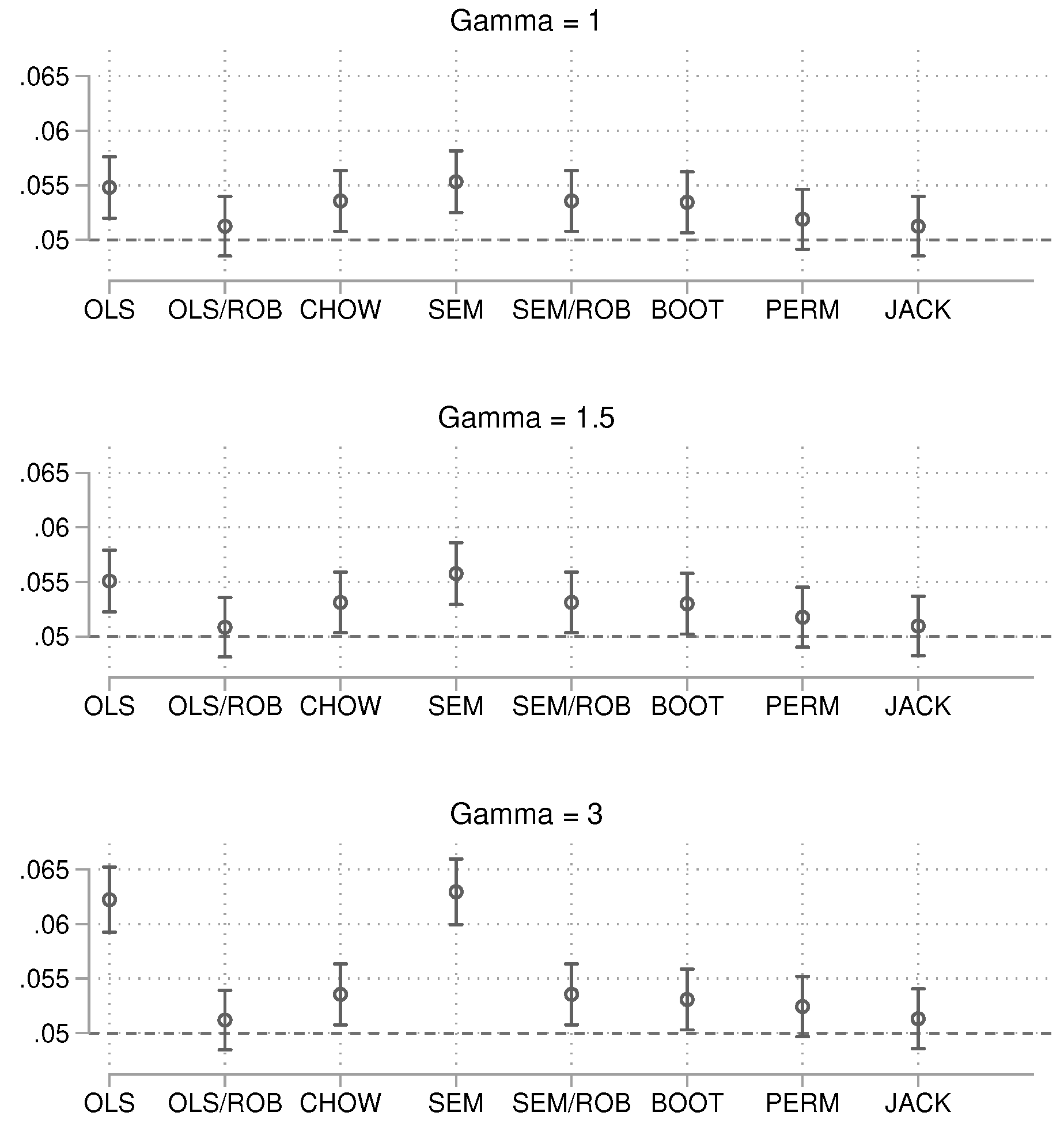
Figure 5.
Probability of producing a p-value smaller than 0.05 in the presence of a true group difference. Total , 15,000 simulations per condition. 95% confidence intervals included.
Figure 5.
Probability of producing a p-value smaller than 0.05 in the presence of a true group difference. Total , 15,000 simulations per condition. 95% confidence intervals included.
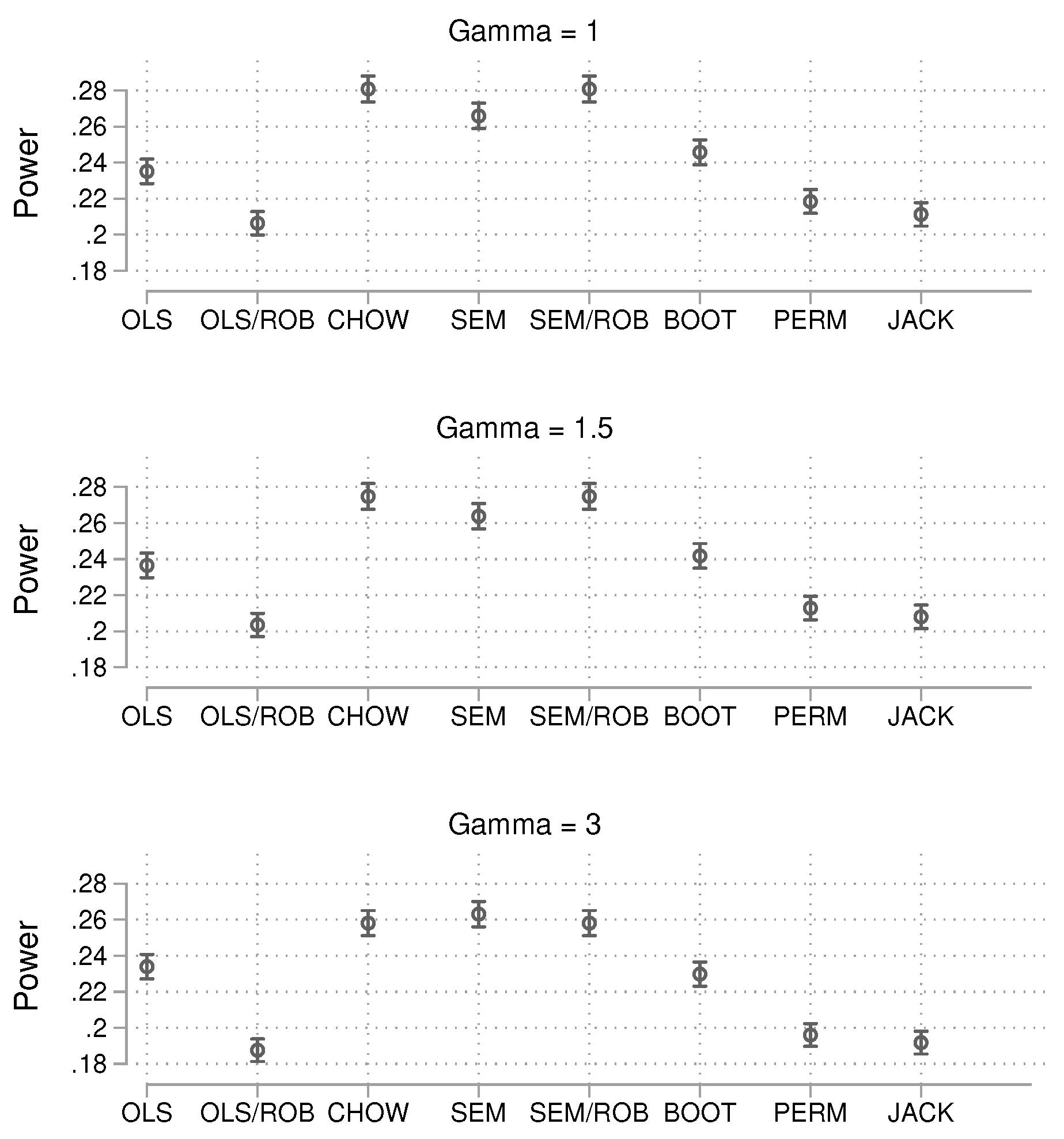
Figure 6.
Probability of producing a p-value smaller than 0.05 in the presence of a true group difference. Total , 15,000 simulations per condition. 95% confidence intervals included.
Figure 6.
Probability of producing a p-value smaller than 0.05 in the presence of a true group difference. Total , 15,000 simulations per condition. 95% confidence intervals included.
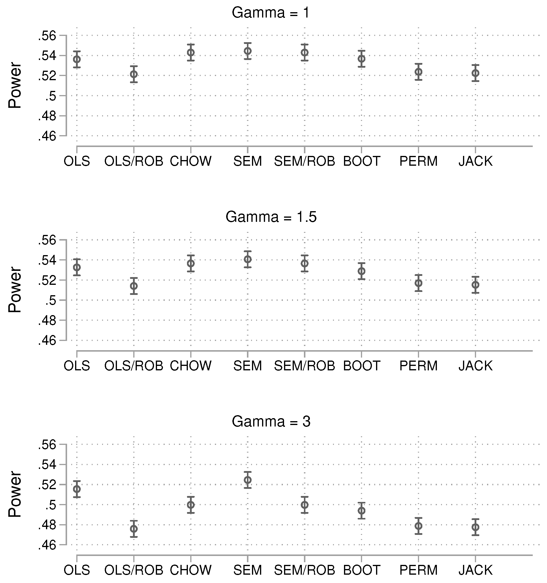
Figure 7.
Probability of producing a p-value smaller than 0.05 in the presence of a true group difference. Total , 15,000 simulations per condition. 95% confidence intervals included.
Figure 7.
Probability of producing a p-value smaller than 0.05 in the presence of a true group difference. Total , 15,000 simulations per condition. 95% confidence intervals included.
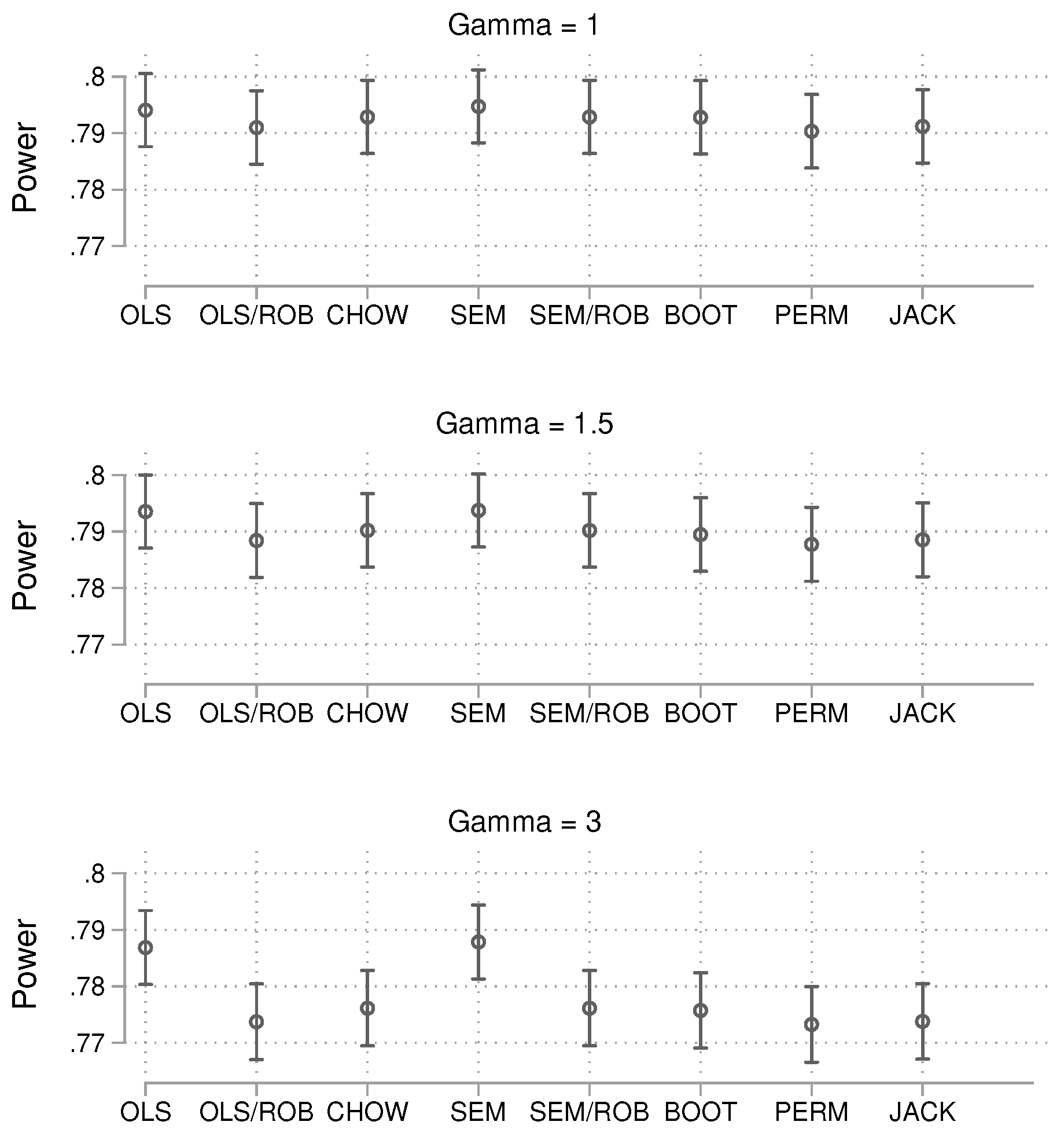
Figure 8.
The x-axis shows the probability of obtaining a p-value smaller than 0.05 in simulations without a true effect, while the y-axis displays the power in simulations with a true effect. Note that the Chow test is numerically identical to the robust SEM approach and is not shown.
Figure 8.
The x-axis shows the probability of obtaining a p-value smaller than 0.05 in simulations without a true effect, while the y-axis displays the power in simulations with a true effect. Note that the Chow test is numerically identical to the robust SEM approach and is not shown.
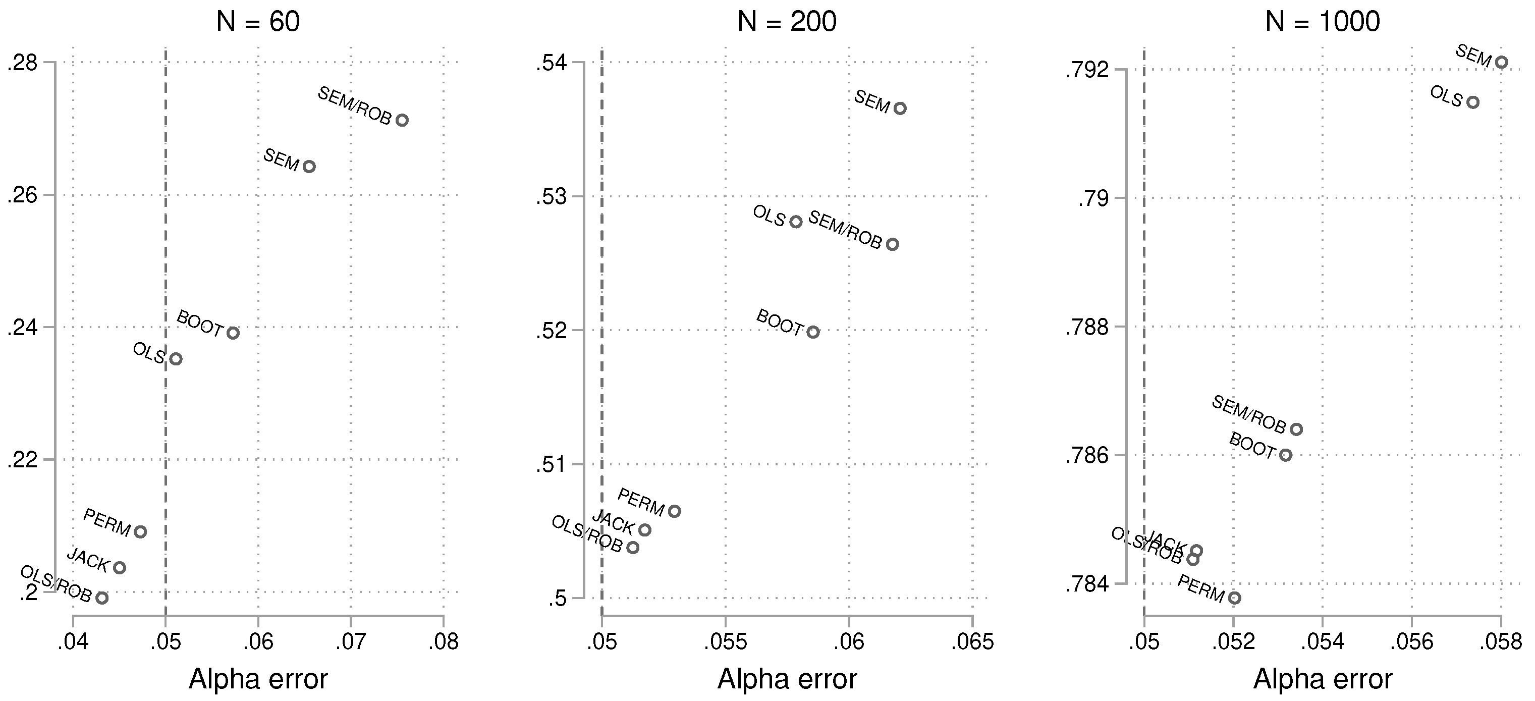
Figure 9.
Probability of obtaining a p-value smaller than 0.05 by method. Total , 25,000 simulations per condition (the realized N is slightly lower due to non-convergence in the small sample/high imbalance condition; 24,872 successful simulations). Confidence intervals are not shown because they are very narrow.
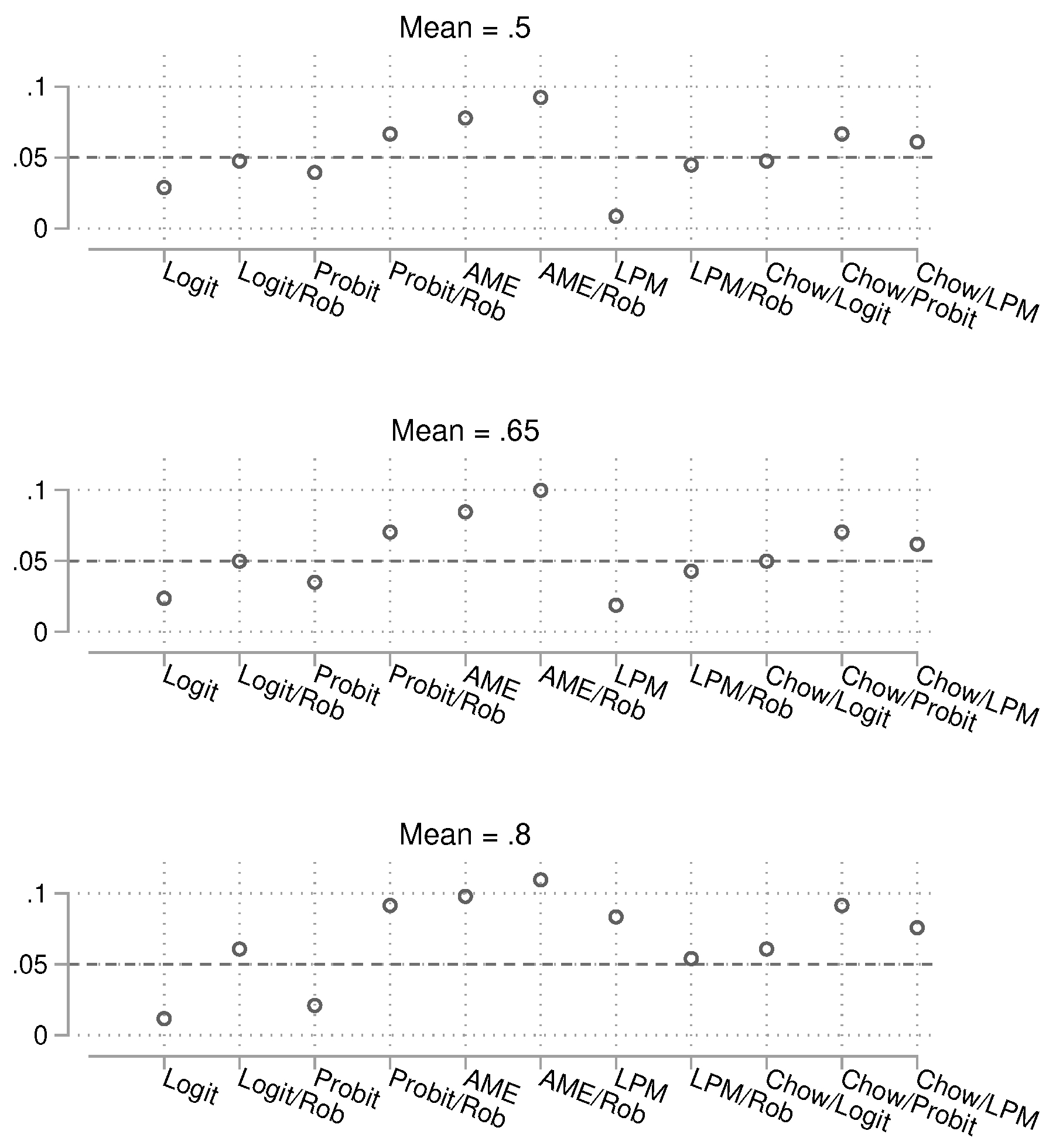
Figure 10.
Probability of obtaining a p-value smaller than 0.05 by method. Total , 25,000 simulations per condition. Confidence intervals are not shown because they are very narrow.
Figure 10.
Probability of obtaining a p-value smaller than 0.05 by method. Total , 25,000 simulations per condition. Confidence intervals are not shown because they are very narrow.
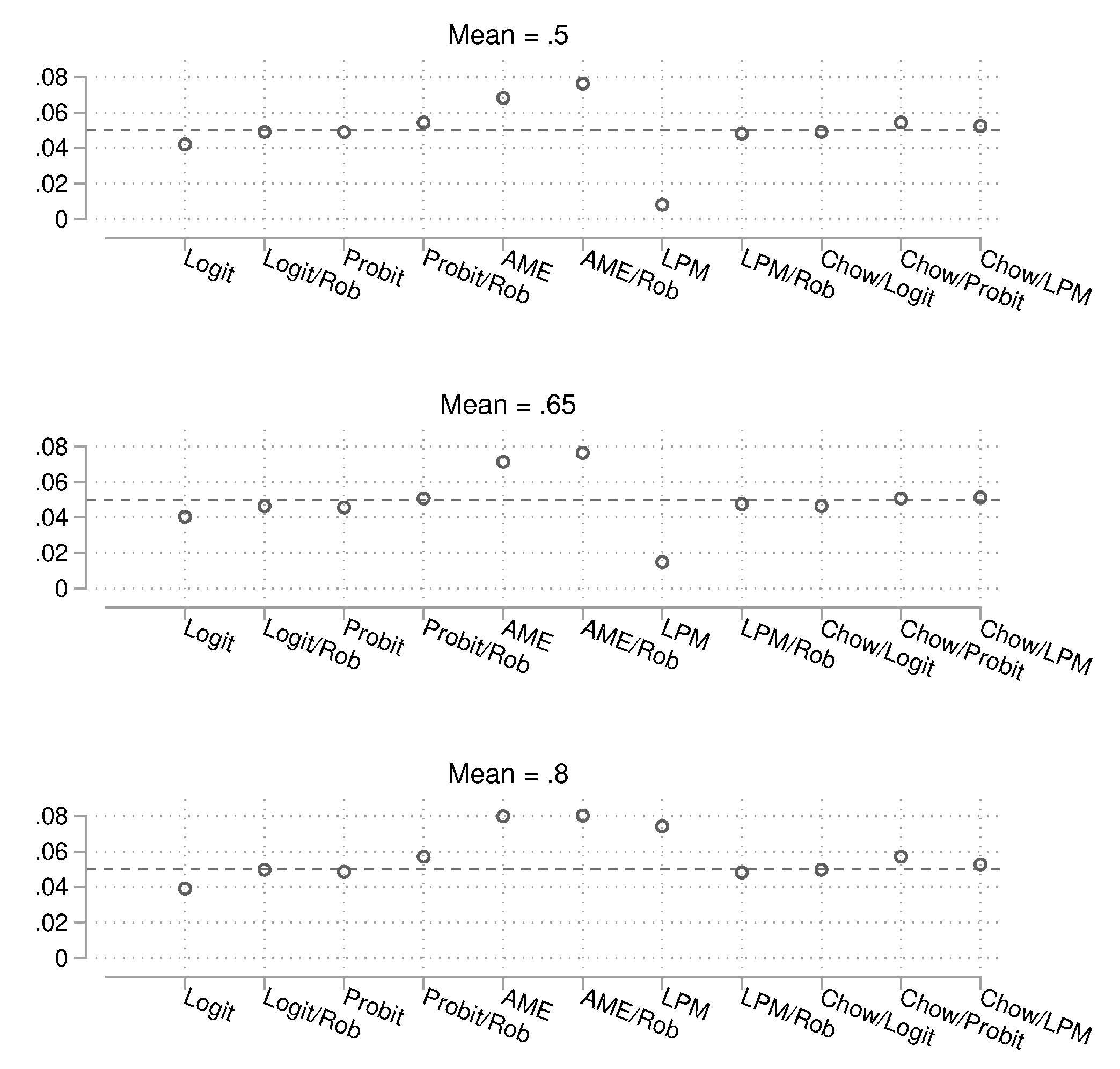
Figure 11.
Probability of obtaining a p-value smaller than 0.05 by method. Total , 25,000 simulations per condition. Confidence intervals are not shown because they are very narrow.
Figure 11.
Probability of obtaining a p-value smaller than 0.05 by method. Total , 25,000 simulations per condition. Confidence intervals are not shown because they are very narrow.
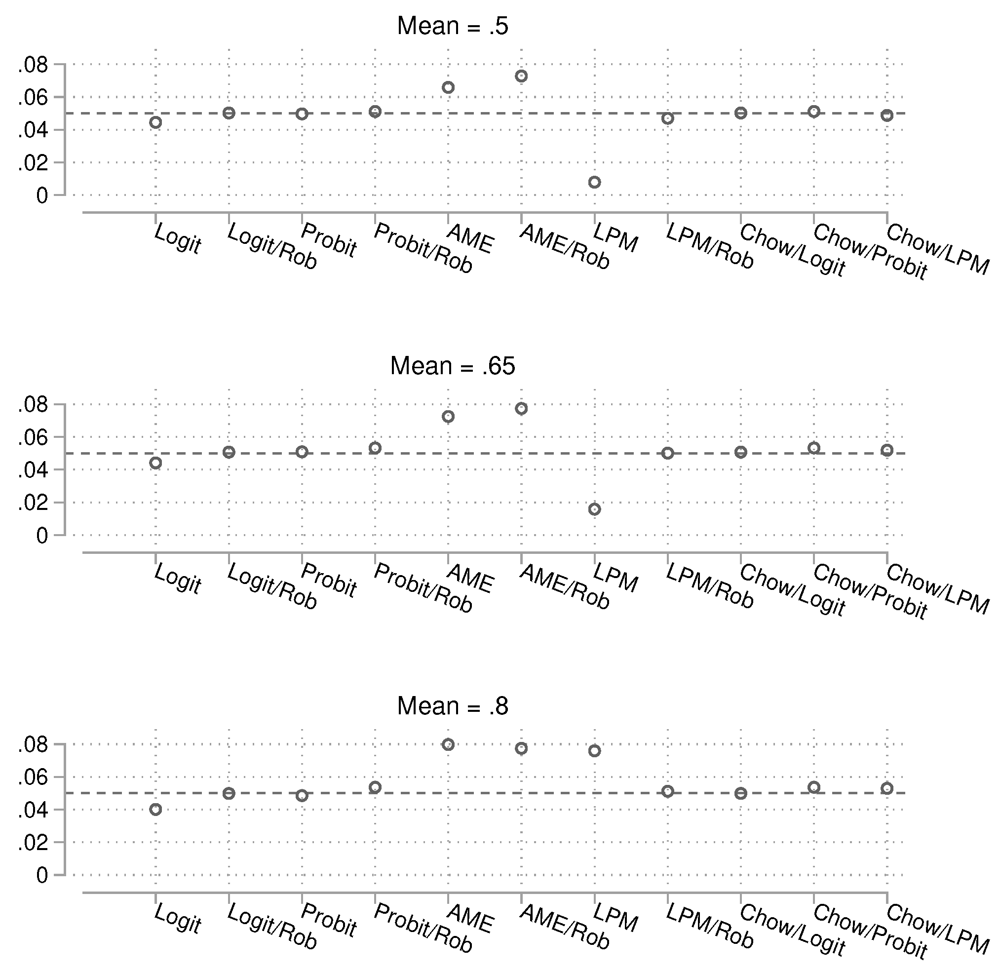
Figure 12.
Probability of obtaining a p-value smaller than 0.05 in the presence of a true group difference. Total , 15,000 simulations per condition. Confidence intervals are not shown because they are very narrow.
Figure 12.
Probability of obtaining a p-value smaller than 0.05 in the presence of a true group difference. Total , 15,000 simulations per condition. Confidence intervals are not shown because they are very narrow.

Figure 13.
Probability of obtaining a p-value smaller than 0.05 in the presence of a true group difference. Total , 15,000 simulations per condition. Confidence intervals are not shown because they are very narrow.
Figure 13.
Probability of obtaining a p-value smaller than 0.05 in the presence of a true group difference. Total , 15,000 simulations per condition. Confidence intervals are not shown because they are very narrow.
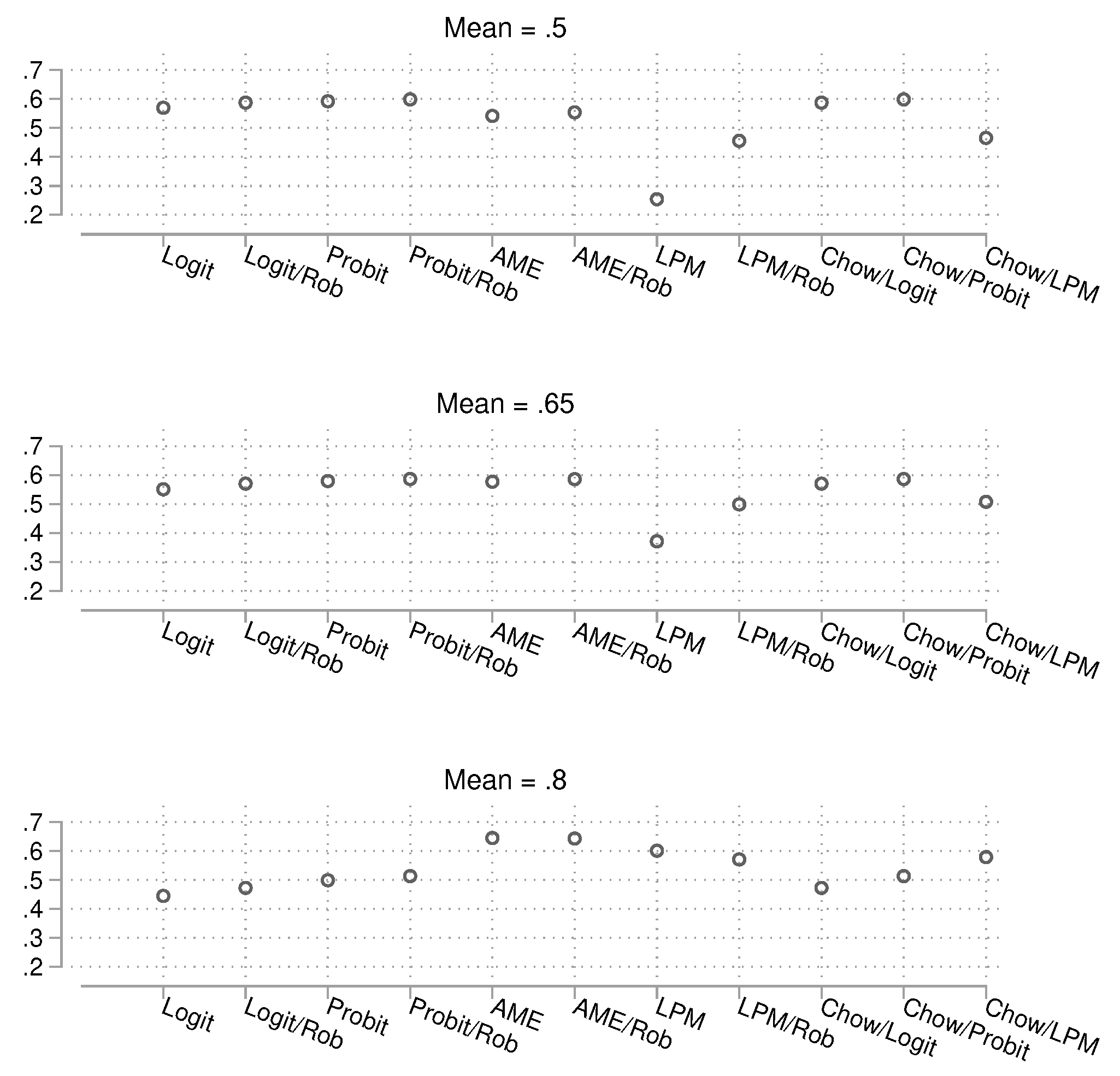
Figure 14.
Probability of obtaining a p-value smaller than 0.05 in the presence of a true group difference. Total , 15,000 simulations per condition. Confidence intervals are not shown because they are very narrow.
Figure 14.
Probability of obtaining a p-value smaller than 0.05 in the presence of a true group difference. Total , 15,000 simulations per condition. Confidence intervals are not shown because they are very narrow.
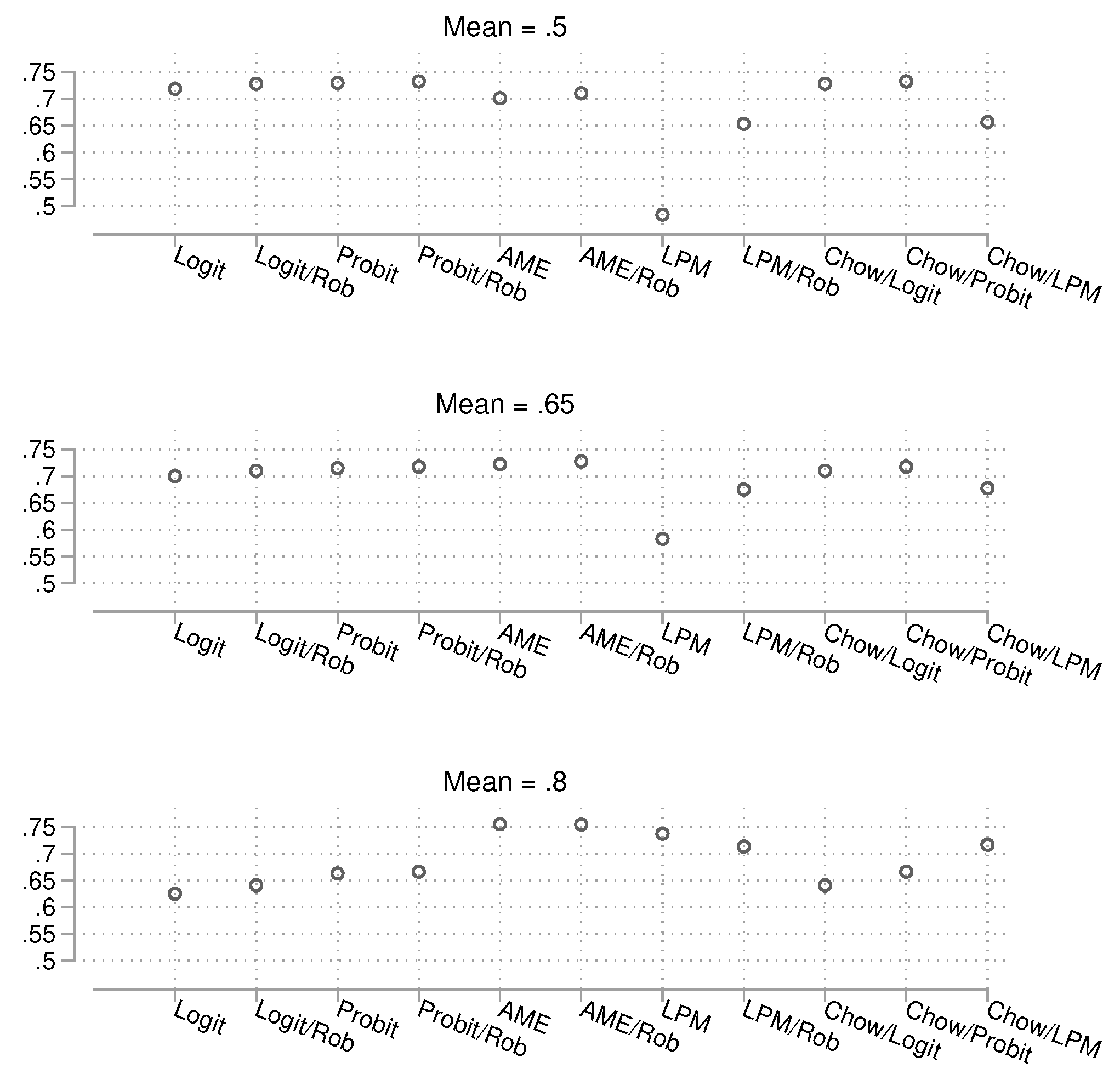
Figure 15.
The x-axis shows the probability of obtaining a p-value smaller than 0.05 in simulations without a true effect, and the y-axis shows the power in simulations with a true effect. Note that the logit Chow test is numerically identical to the robust logit, and the probit Chow test is equivalent to the robust probit.
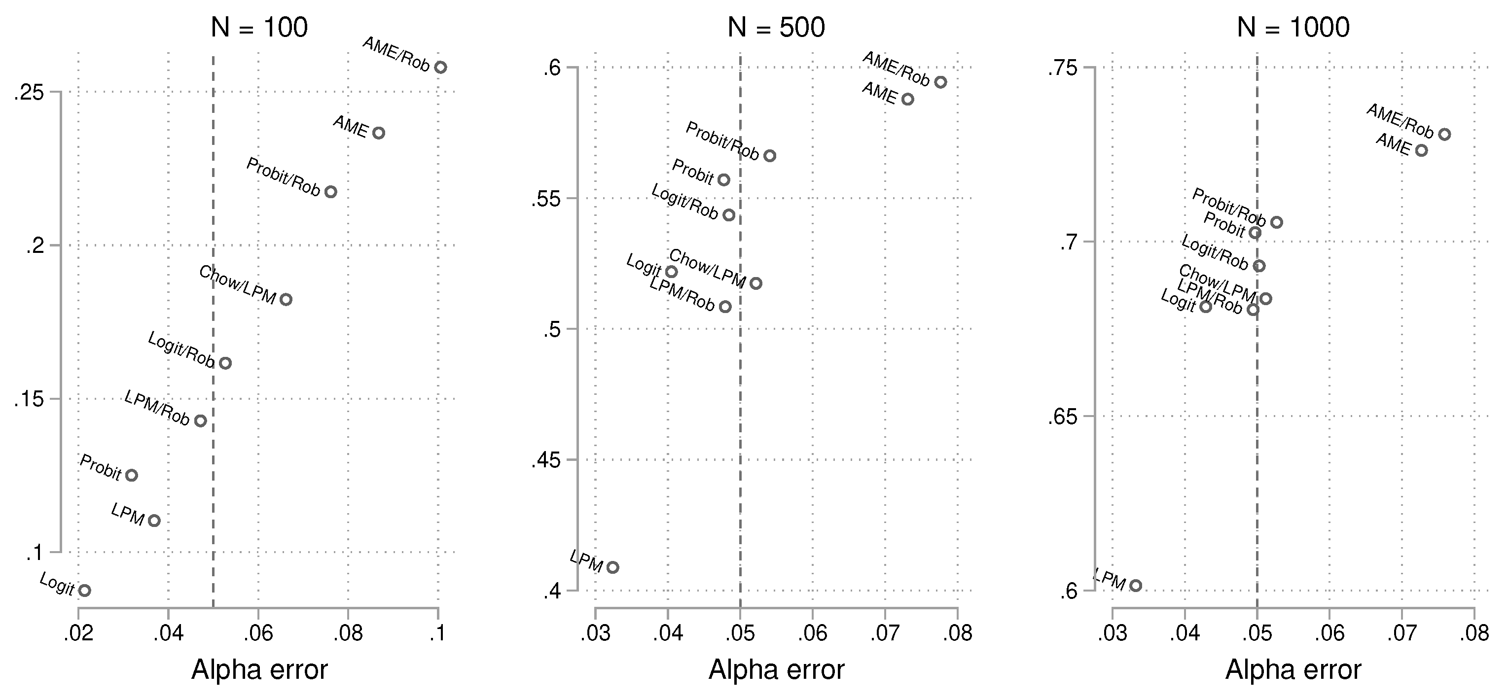
Figure 16.
While logit picks up nonlinear effects automatically, regress does not. In both cases, having a better modeling approach with higher-order terms improves the prediction.
Figure 16.
While logit picks up nonlinear effects automatically, regress does not. In both cases, having a better modeling approach with higher-order terms improves the prediction.
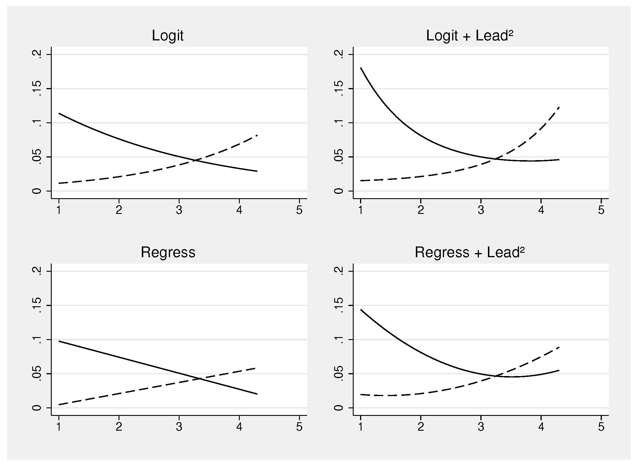
Table 1.
Overview of all methods for continuous outcome variables.
| Pooled OLS | Chow | SEM | Bootstrap | Jackknife | Permutation | |
|---|---|---|---|---|---|---|
| P-value | Yes | Yes | Yes | Yes | Yes | Yes |
| SE/CI | Yes | Yes | Yes | |||
| Robustness | / | |||||
| Missing data | MICE | FIML a | (MICE) | |||
| Runtime b | 1 | 3.6 | 3.3 | 755 | 492 | 329 |
a Only works if there are no missing values on the group variable. b Computed for a sample size of 1,000 using asreg to speed up the nonparametric methods. 1,000 bootstrap/permutation resamples. OLS normed to be 1 (100%). c The robust SEM approach is numerically equivalent to the Chow test.
Disclaimer/Publisher’s Note: The statements, opinions and data contained in all publications are solely those of the individual author(s) and contributor(s) and not of MDPI and/or the editor(s). MDPI and/or the editor(s) disclaim responsibility for any injury to people or property resulting from any ideas, methods, instructions or products referred to in the content. |
© 2024 by the authors. Licensee MDPI, Basel, Switzerland. This article is an open access article distributed under the terms and conditions of the Creative Commons Attribution (CC BY) license (http://creativecommons.org/licenses/by/4.0/).
Copyright: This open access article is published under a Creative Commons CC BY 4.0 license, which permit the free download, distribution, and reuse, provided that the author and preprint are cited in any reuse.


