
Submitted:
03 January 2025
Posted:
06 January 2025
You are already at the latest version
Abstract
Wildfires impact human health, air quality, visibility, weather, climate change and cause huge economic losses. Although air quality monitors operated by state and counties can provide insights about unhealthy air quality during wildfires, these monitors are not available everywhere. It is important to design affordable tools that anyone from the general public could use to diagnose air quality impacts. We apply machine learning with deep neural networks to rapidly diagnose air quality from images of the sky taken at a ground site at the Pacific Northwest National Laboratory in Richland, WA, USA. We train a deep neural network model using convolutional neural network frameworks to diagnose air quality indices from sky images. Our work demonstrates the application of a complex deep learning framework on a small dataset of new sky images through the use of transfer learning, which leverages previously determined weights and biases of the model and fine tunes it to a new dataset, greatly reducing the time for training the model. Rapid diagnosis of air quality during wildfire episodes could provide early warning to the public and aid in applying timely mitigation strategies against acute smoke exposure, especially for vulnerable populations. We also show that the risk of lower respiratory infection is the greatest for human health at acute smoke exposures, and reactive oxygen species exposure associated with wildfire particles could cause various inflammation and health risks.
Keywords:
wildfires
; machine learning
; total sky imager
; neural networks
; air quality
; climate
; human health
1. Introduction
Wildfire activity (both the frequency and durations of large wildfires) has been increasing in recent decades[1] in many regions globally including the Western United States due to climate change and expanding human activity. Fires emit hazardous air pollutants including PM2.5, carbon monoxide and volatile organic compounds which could affect human and ecosystem health[2,3,4], and the Earth’s radiative forcing[5]. Ultra-fine particles (particles with diameters less than 50 nm) formed by atmospheric chemical aging of gases emitted by smoke were recently shown to intensify deep clouds and heavy precipitation thereby affecting weather and climate systems[6]. Wildfire smoke could travel thousands of miles in the atmosphere affecting large regions and communities. In order to assess compliance with National Ambient Air Quality Standard (NAAQS), the Environmental Protection Agency (EPA) collects air quality monitoring data in collaboration with state, local and tribal agencies and makes such data publicly available [7]. Fine particles (PM2.5, particles with diameters less than 2.5 ) associated with wildfire smoke could greatly impact human mortality and diseases including lower respiratory infection, chronic obstructive pulmonary diseases (COPD) and lung cancer [8]. Epidemiological studies indicate that reactive oxygen species (ROS) associated with chemicals in wildfire smoke particles like polycyclic aromatic hydrocarbons and transition metals could cause cardiovascular impairment, which may be responsible for two-thirds of human mortality rate due to air pollution [9].
Acute exposure to wildfire smoke might reduce several of the benefits of controlling sources of human-caused air pollution. Therefore, it is important to continuously monitor air pollution including PM2.5, especially in vulnerable communities, globally. However traditional sensors for air quality monitoring are often expensive and require specialized skills to operate making their application impractical over large regions of interest, especially for vulnerable communities that are affected by air pollution. This creates a need for developing fast, accessible, low-cost detection methods of air quality that could create early-warning systems for poor air quality. Such warning systems of outdoor air quality could help people make informed decisions about their health and safety when wildfires occur.
In this work, we apply machine learning using deep convolutional neural networks to rapidly diagnose air quality by combining hourly air quality monitoring data PM2.5 from the Washington State Department of Ecology [10] with the local images of the sky collected by the total sky imager (TSI) [11] at the Pacific Northwest National Laboratory in Richland, WA USA located at 46.34°N, 119.27°W. Using a transfer learning approach, we adapt a deep neural network to rapidly detect air quality indices (AQI) just from a relatively small set of sky image datasets. Our approach could be widely used to rapidly detect air quality, especially during intense wildfires, providing an economical approach that could likely provide early warning to public, thereby enabling timely application of mitigation strategies to reduce health risks from smoke exposure. In addition, we calculate the health risk of PM2.5 using 2 approaches: (1) Integrated exposure-response functions that relate PM2.5 to health endpoints (2) Calculation of ROS potential during and after smoke influence. Our results highlight the large increase in health risks during wildfire smoke influence.
2. Materials and Methods
During September 2020 wildfires burnt in Oregon WA, and the wildfire smoke was transported for hundreds of kilometers in the atmosphere. At a local site in Kennewick, WA PM2.5 concentrations were measured hourly and daily averaged PM2.5 exceeded 200 ) as shown in Figure 5, and discussed in more details later. Our goal in this study is to develop a cost-effective air quality detection method, especially during heavy pollution episodes such as intense wildfires, which can be used by the general public. To achieve this, we leverage two key datasets over a site in WA, USA during and after intense wildfires of September 2020: (1) Air quality indices derived from hourly measurements of PM2.5 taken from the Washington State Department of Ecology [12] at Kennewick, WA (2) Hourly daytime images of the sky generated by a total sky imager (TSI) [13] at the Pacific Northwest National Laboratory (less than 15 miles from the Kennewick, WA site). Air quality indices are categorized based on PM2.5 concentrations as: Class 1, Good (1 ≥ PM2.5≤ 12 ), Class 2, Moderate (12.1 ≥ PM2.5≤ 35.4 ), Class 3, Unhealthy (55.5 ≥ PM2.5≤ 150.4 ), and Class 4, Very unhealthy (150.5 ≥ PM2.5≤ 250.4 ) during Sep 10-20, 2020. During the daytime when the TSI takes sky images, we have about 15 images each in the Good and Moderate AQI classes, about 30 images in the unhealthy and 46 images in the very unhealthy class, that provides an overall dataset of a total of 104 sky images. We then train a supervised machine learning model that classifies the TSI images into the above defined 4 different air quality categories by directly relating them at a given time to the measured air quality based on the corresponding PM2.5 measurements. Although the dataset is very small for training a deep learning model (that requires thousands of images), we demonstrate the utility of "transfer learning" approach that leverages a previously trained MobileNetv2 modeling framework as we discuss later.
Here, we provide a brief description of measurement methods for PM2.5 and sky image datasets used in our study. The Beta Attenuation Monitors (BAM) instruments are Federal Equivalent Method (FEM) monitors used by the WA Department of Ecology to measure PM2.5 concentrations in near-real-time for regulatory and public information purposes[12]. The total sky imager (TSI) operated by the Pacific Northwest National Laboratory at Richland WA, USA, captures time series of hemispheric images of the sky during the daylight hours using a solid state CCD imaging camera that overlooks a heated hemispherical mirror [13]. The mirror projects the hemispherical sky image into the lens, and has a solar-ephemeris guided shadow-band to block the direct solar radiation (that can damage the instrument). An image-processing code running on a user-provided computer captures these images at user-defined sampling rates (usually hourly) and saves them to JPEG files for analysis.
To efficiently train a state-of-the-art machine learning model with the limited air quality data during wildfire influence (few days), we leverage transfer learning based on the MobileNetv2 framework [14]. MobileNetV2 was initially trained on the ImageNet (ILSVRC-2012) dataset, which contains approximately 1.2 million images spanning 1,000 categories. Through this extensive training, the network learns diverse feature representations—such as edges, textures, and shapes—across various object classes. Consequently, when the MobileNetV2 framework adapts to a new smaller dataset, it can leverage these previously learned representations, reducing the required training time and data volume while still maintaining high accuracy. However the original dataset used to train MobileNetv2 did not use a TSI dataset or air quality indices for its classification. We demonstrate the utility of using "transfer learning". Transfer learning involves freezing (freezing refers to making sure the previously trained weights and biases of its layers are used as they are and not trainable) the weights and biases of the convolutional layers (A layer in machine learning is a structural component in which specific computations are performed on input data to produce an output) determined by MobileNetV2 through training the dataset of 1.2 million images. We adapted the MobileNetv2 model for classifying our TSI images according to the 4 air quality categories (Good, Moderate, Unhealthy and Very unhealthy as described above). For this, we added 2 trainable layers at the end of its previously trained layers. Note that a neuron is a unit of computation in a neural network takes one or more inputs, processes them, and produces an output. Our added layer 1 consists of 1024 neurons with Relu activation, while layer 2 consists of 4 neurons with softmax probabilities corresponding to each of our 4 Air quality classes. The output of the 2nd added layer represents the probability that a given sky image corresponds to the 4 air quality classes, and the maximum of these 4 probabilities determines the air quality index that a given image belongs. We developed our transfer learning code to train the MobileNetv2 model using the Google Colab platform [15]. Our trained model, posted on github [16] can be easily run from any local computer to predict air quality from new sky images, and represents a quick, computationally efficient and publicly accessible way to diagnose air quality and provide timely warning to the public.
3. Results
Our dataset comprises a total of 104 images that we split into a training set and a validation set with 80% of the images used in training and 20% used in validation. Splitting a portion of the data to be used as a validation set enables evaluating intermediate model performance during training and guide hyper-parameter tuning, helping to prevent over-fitting on the training data [17]. Due to the limited size of our training data, we also used Keras’s ImageDataGenerator function [18] to augment our training dataset during training e.g. by using horizontal flip, shear (shearing refers to simulating horizontal/vertical skews and distortions to the images in order to increase generalizability) and zoom. For each epoch (an epoch is one pass of the model over the entire training data) of training the ImageDataGenerator function might generate around 64 augmented images (calculated based on our specified batch size of 32 and number of training images), stored only in the memory during training (not saved), for a total of 1920 images (since we train for 30 epochs). On each epoch, the generator either reuses some of the previous images from memory or augments them with new ones.
We first froze the default layers of MobileNetv2. Often, in deep neural network architectures like the MobileNetv2, the last step involves a fully connected layer called the “top layer”, which takes all the high-level features extracted by earlier convolutional (or other feature-extraction) layers and maps them into final outputs (such as class scores in a classification problem). Since each neuron in this fully connected layer links to every neuron in the preceding layer, it effectively combines all learned representations into a single predictive distribution.
In order to adapt the MobileNetv2 model to our new datasets, we replaced the top fully connected layer in MobileNetv2 with a new trainable fully connected layer of 1024 neurons involving ReLu activation. Adding another trainable fully connected layer with 4 neurons and softmax probabilities we applied these for generating probabilities that sum to 1 corresponding to our 4 AQI classes. Softmax is a function that transforms a vector of real-valued scores into a probability distribution where the sum of probabilities is 1. These 2 layers that we added can be trained with our new dataset, thus using "transfer learning" i.e. fine tuning the MobileNetv2 model to our new dataset.
Next we used the Adam optimizer with the categorical cross entropy loss, a widely used loss function in machine learning, especially for classification tasks. Categorical cross entropy measures the difference between the predicted probability distribution produced by the model and the true distribution (AQI class labels in our study). The training data is shuffled ensuring that the model sees the data in different orders each epoch, preventing over-fitting the model to a specific order or a distribution of batches per epoch improving its generalizability. Since we used transfer learning, we chose a small learning rate of 0.0001 to avoid drastic parameter tuning (weight updates) [19], allowing the model to gradually adapt and generalize well to our new task of relating AQI classes to our sky image datasets.
Figure 1 is an example of of the 4 classes of air quality indices shown as good, moderate, unhealthy, and very unhealthy determined from PM2.5 measurements by WA department of Ecology and the corresponding TSI images of the sky captured at PNNL.
3.1. Training the Model
Since we froze the convolutional layers of the MobileNetv2 model, the process of training via "transfer learning" only determines the parameters (weights and biases) of the top two layers that we added to fine tune the model to our sky image dataset. Figure 2 shows that the model demonstrates rapid convergence, with both training and validation accuracies rising quickly from lower initial values to over 90%.
3.1.1. Discussing Model Performance
Figure 2a presents the evolution of both accuracy and loss over 30 training epochs. As seen in panel (a), training accuracy starts at roughly 42% and increases to about 92% by the final epoch. The validation accuracy likewise improves from around 57% to 91%. This nearly parallel rise in accuracies indicates consistent learning across training and validation sets, with no strong evidence of over-fitting.
Panel (b) shows the corresponding training and validation loss curves. Training loss decreases from about 1.24 to 0.26, while validation loss declines from about 1.10 to 0.33. Both curves follow a similar downward trend, reinforcing the idea that the model is learning features rather than memorizing the training data. Moreover, the relatively small gap between training and validation metrics underscores the model’s generalization capabilities within the dataset.
Overall, these results suggest that the network architecture, along with the parameters, effectively learns to classify the data while keeping a stable performance on the validation set. The convergence of the training and validation curves by the final epochs indicates that the training procedure achieved a good balance between under-fitting and over-fitting, which is reflected in high accuracy and low loss for both training and validation datasets. Importantly, we do not see the typical signature of over-fitting (limited generalizability) indicated by instances of training loss decreasing but validation loss increasing rise. Our results are highly encouraging, as they demonstrate rapid learning and sustained improvement without major divergences between training and validation curves. While the high validation performance is promising, it would be helpful to test the model with more unseen images to confirm the true extent of the model’s capabilities.
3.1.2. Testing the Model
Figure 3 demonstrates the testing of our trained model on example images from the validation set (not used for model training), where a random image is chosen from each of the 4 AQI classes. Since we also have corresponding PM2.5 concentrations, we know the true AQI class that the image belongs to, thereby allowing evaluation of the model predicted AQI class with ground truth measurements.
In addition, we also tested the model on a completely unseen dataset during wildfires in 2018 that were never used in training or validation. As described earlier, when a new sky image is provided as an input to our trained model, it outputs probabilities that the new image belongs to each of the 4 AQI classes with these probabilities summing to 1. The maximum value of these 4 probabilities determine which AQI class (Good, Moderate, Unhealthy, Very Unhealthy) the new test image most likely belongs to. In Figure 3, the tallest bar (maximum softmax probability shown on Y-axis) among the 4 grouped vertical colored bars for each image (X-axis) represents the model predicted AQI class for that image. From left to right on X-axis, we chose images with known AQI classifications with their known AQI levels ranging "Good" to "very unhealthy". The trained MobileNetv2 model successfully determines the maximum probabilities and AQI classifications for Good (green , 86%), Moderate (yellow, 60%), Unhealthy (red, 85%) and Very unhealthy (purple, 75%) in agreement with the known AQI classifications of these images. The fifth rightmost image (on X-axis) represents a completely unseen image from another year (August 2018 wildfires) that was not used in model training or validation sets. Based on measured PM2.5 concentrations during that time, this image belongs to Unhealthy class. The model succesfully determines that this image corresponds to unhealthy AQI levels, assigning an estimate 62% probability to unhealthy and 36% probability to very unhealthy AQI. Although PM2.5 concentrations during both 2018 and 2020 wildfires might indicate a given AQI level (Unhealthy, Very unhealthy), the color and visibility of sky might differ due differences in vegetation burnt, atmospheric transport and chemical aging of smoke. The smoke in 2020 encountered at Kennewick was generated by vegetation burnt in Oregon, while the 2018 smoke was transported from Canada. In addition, the 2020 smoke (wildfires burning in Oregon, WA) encountered at Kennewick traveled through shorter transport distances and aging compared to 2018 smoke (burning in Canada) was not used for model training and validation, a reduced model performance is expected especially due to differences in smoke. However, the model trained on 2020 data still identified unhealthy AQI during 2018 smoke influence, corroborated by local PM2.5 measurements, providing confidence in applicability of our model to identify smoke episodes from sky images. Model performance could be increased by including the 2018 data in model training in addition to 2020 data. However, our objective here was to demonstrate the generalizability of the model on completely unseen datasets such as the 2018 wildfire episode.
3.2. Health Impacts of Smoke
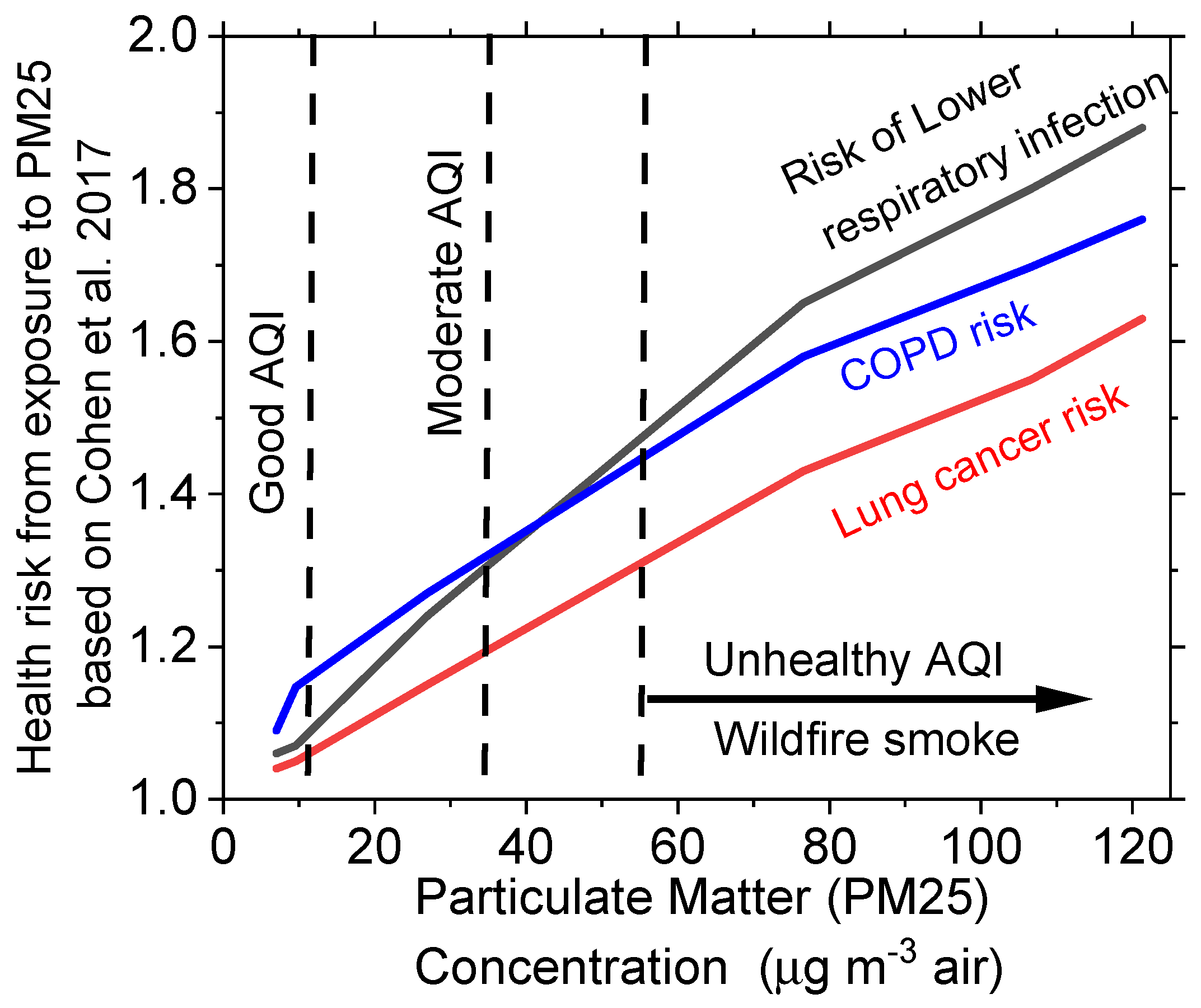
Exposure to ambient air pollution is a leading contributor to the global burden of disease and causes mortality and morbidity. Based on epidemiological studies using non-linear exposure–response functions spanning the global range of exposure, Cohen et al. [8] estimated the relative risks of mortality from respiratory diseases and lung cancer attributable to PM2.5 and presented trends in global burden of disease from 1990 to 2015. Based on a growing body of international studies, they highlighted that ambient air pollution and its associated burden of disease can be lowered via policy actions that control sources of PM2.5. However, uncontrolled wildfires generate substantial air pollution including PM2.5 that could reduce the benefits of policy actions designed to reduce the impacts of human activities on air pollution. Figure 4 illustrates the relationship between PM2.5 concentrations measured during the Sep 2020 wildfires in Kennewick, WA and corresponding AQI levels with relative health risks, normalized to a baseline value of 1.0. The bottom three panels of Figure 1 from Cohen et al. [8] were used to compare health risks associated with PM2.5 concentrations related to three different causes of death: lower respiratory infections, lung cancer, and chronic obstructive pulmonary disease (COPD) for all ages in Kennewick, WA. Health risks were directly estimated by reading the risk values corresponding to PM2.5 concentrations observed in Kennewick WA from the graphs in Cohen et al.[8].
The three curves demonstrate a non-linear increase in health risks with rising PM2.5 concentrations, with the risk of lower respiratory infections exhibiting the steepest growth, followed by COPD and lung cancer. Vertical dashed lines AQI categories ("Good," "Moderate," and "Unhealthy"), indicating thresholds of concern for air pollution exposure. Figure 4 highlight the significant public health impacts of air pollution. Importantly, Figure 4 shows that even AQI levels classified as Good might exceed the relative risk of 1.0. COPD risk is higher than the risk of lower respiratory infection and lung cancer risk at good to moderate AQI levels, however, the risk of lower respiratory infection shows the steepest increase with the increase in PM2.5 levels. During wildfire smoke episodes, when the air quality is unhealthy at PM2.5 exceeding 55 , the risk of lower respiratory infection presents the greatest relative risk as the most significant cause of death. This figure serves as a valuable framework for estimating health risks based on observed PM2.5 concentrations in specific geographic regions like Kennewick as included in our study.
3.2.1. Reactive Oxygen Species Associated with PM 2.5 in Wildfire Smoke
The short-term acute health effects associated with high reactive oxygen species (ROS) associated with PM2.5 during wildfire events are a critical concern. Elevated ROS levels can exacerbate oxidative stress, leading to inflammation, respiratory distress, and cardiovascular strain[9]. Vulnerable populations, such as individuals with pre-existing respiratory or cardiovascular conditions, are particularly at risk during such events.
Figure 5 shows the temporal variation of daily averaged PM2.5 concentrations (bars and left Y-axis) and the associated reactive oxygen species (ROS) potential during the September 2020 wildfires in Kennewick, WA, revealing critical public health implications. ROS potential (line and right Y-axis in Figure 5) is calculated by multiplying PM2.5 concentrations with the oxidative potential (OP) using the value of 0.069 nmol/min/g for biomass burning [20]. Combustion conditions affect the OP for wildfire generated particles, such that flaming (OP ~0.12 nmol/min/g) generates higher OP compared to smoldering conditions (OP ~0.03 nmol/min/g) [21]. For urban background and traffic influenced sites the OP ranged ~0.08 to 0.13 nmol/min/g, calculated by normalizing the OPDTT values with corresponding PM2.5 concentrations in Janssen et al. [22]. In this work, we used a constant OP value of 0.07 for estimating ROS content in Kennewick, WA since the site is influenced by urban traffic and other background sources in addition to wildfire smoke during smoke episodes.
Figure 5.
ROS potential calculated from PM2.5 concentrations and a constant assumed OP value as described in the text.
Figure 5.
ROS potential calculated from PM2.5 concentrations and a constant assumed OP value as described in the text.
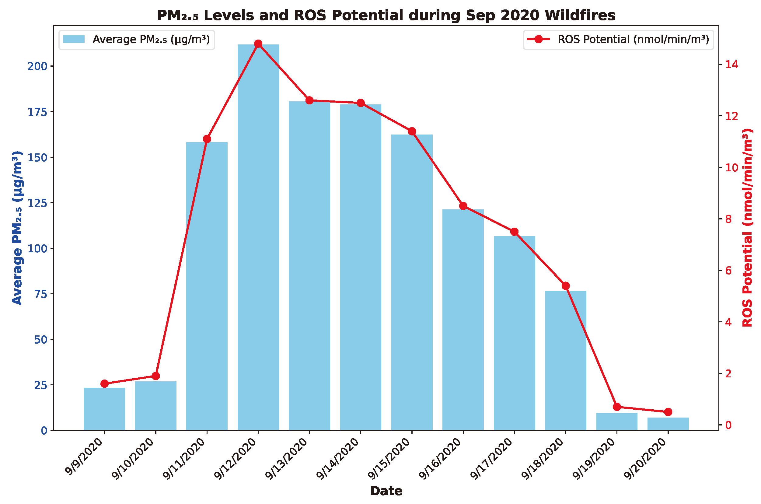
The redox active nature of biomass burning emissions and other combustion sources is caused by the presence of polycyclic aromatic hydrocarbons (PAHs), and transition metals in PM2.5. Our results highlight the large contribution of wildfire-derived PM2.5 to oxidative stress compared to baseline air pollution, mainly due to high PM2.5 concentrations of wildfire smoke compared to background sources. For example, Figure 5 shows that the daily averaged ROS potential was ~30 times higher during intense wildfire day of Sep 12, 2020 (14.8 nmol/min/m3) compared to the ROS potential on the clean background day of Sep 20, 2020 of 0.5 nmol/min/m3 in Kennewick, WA. This highlights the significant oxidative stress burden posed by wildfire smoke.
Notably, even as PM2.5 levels declined after September 15, 2020, the ROS potential remained elevated, likely sustained by secondary aerosol formation due to atmospheric chemical processing of smoke gases and particulate matter. Future work should investigate the chemical drivers of ROS potential and the role of atmospheric aging in sustaining health risks associated with wildfire smoke.
4. Discussions
Wildfires are one of the largest natural sources of air pollution that might significantly lower the benefits of pollution control policies, globally. Smoke from wildfires travels thousands of miles in the atmosphere, and could cause short-term and acute human exposures to pollutants including PM2.5 causing health risks include mortality and morbidity in humans. Timely ground-based detection of acute smoke exposure is of critical importance in all regions where there is significant human inhabitancy, so that smoke exposure and its health impacts can be effectively mitigated. However, continuous and widespread PM2.5 monitoring might be expensive and impractical, especially in developing regions, and its important to develop affordable methods of smoke detection.
In this work, we used a deep neural network machine learning framework to predict air quality indices by relating images of the sky with AQI diagnosed through PM2.5 measurements at a local site in Kennewick, WA. By leveraging "transfer learning", we also demonstrated a computationally efficient approach to adapt a pre-trained complex deep convolutional neural network model (MobileNetv2) to our completely new datasets (sky images and AQI indices). Despite a small amount of sky image data (a total of 104 images collected hourly during the 10-day period of Sep 10-20, 2020 daytime), our transfer learning approach with data augmentation produced high training and validation accuracy over just 30 epochs of training and performed well on test images from the validation data in Sep 2020. Our model also successfully predicted unhealthy levels of AQI during intense wildfires of August 2018, using these completely unseen test images that were never used in training and validation (our model was only trained on Sep 2020 dataset). Our machine learning approach has tremendous promise in rapidly diagnosing AQI just from sky images that could be taken at locations of interest worldwide. In the absence of more expensive PM2.5 measurements (e.g. in urban neighborhoods within developing countries devoid of monitoring infrastructure), we provide a viable alternative to provide timely estimates of AQI for public health advisories and policy actions that could provide clean air shelters, and other interventions to mitigate human exposure and reduce health risks during wildfire episodes. Our trained model in google colab platform can be easily run from any local computer to predict air quality from sky images by policymakers and general public.
In addition, we showed that the risk of lower respiratory infections is likely the greatest risk of mortality during short term acute exposures to smoke. Our study also shows that acute exposures to wildfire smoke could cause more than an order of magnitude higher reactive oxygen species exposure compared to cleaner periods, which could lead to inflammation, respiratory distress, and cardiovascular strain, especially in vulnerable populations.
Author Contributions
A.M.S. conceptualized this work, analyzed the PM2.5 measurement data and related these to TSI sky image dataset, and conducted formal analyses including the development, running and testing of the deep learning model, and also wrote the original draft of the Manuscript, M.S. contributed to the validation of the software and the results, generating visualizations, and review and editing of the Manuscript drafts.
Funding
M.S. acknowledges support by the US Department of Energy (DOE) Office of Science, Office of Biological and Environmental Research (BER) through the Early Career Research Program. The Pacific Northwest National Laboratory (PNNL) is operated for the DOE by Battelle Memorial Institute under contract DE-AC06-76RL01830.
Data Availability Statement
Acknowledgments
The authors gratefully acknowledge Susanne Glienke at the Pacific Northwest National Laboratory (PNNL) for curating the TSI sky image dataset used in this work, and Evgueni Kassianov at PNNL for helpful discussions.
Conflicts of Interest
The authors declare no conflicts of interest.
References
- Westerling, A.L.; Hidalgo, H.G.; Cayan, D.R.; Swetnam, T.W. Warming and Earlier Spring Increase Western U.S. Forest Wildfire Activity. Science 2006, 313, 940–943. [Google Scholar] [CrossRef]
- Urbanski, S.P.; Hao, W.M.; Baker, S. Chemical composition of wildland fire emissions. Developments in Environmental Science 2008, 8, 79–107. [Google Scholar]
- Cascio, W.E. Wildland fire smoke and human health. Science of The Total Environment 2018, 624, 586–595. [Google Scholar] [CrossRef] [PubMed]
- Andreae, M.O. Emission of trace gases and aerosols from biomass burning—An updated assessment. Atmospheric Chemistry and Physics 2019, 19, 8523–8546. [Google Scholar] [CrossRef]
- Ward, D.S.; Mahowald, N.M.; Kloster, S. The changing radiative forcing of fires: global model estimates for past, present, and future. Atmospheric Chemistry and Physics 2012, 12, 10857–10886. [Google Scholar] [CrossRef]
- Shrivastava, M.; Fan, J.; Zhang, Y.; Rasool, Q.Z.; Zhao, B.; Shen, J.; Pierce, J.R.; Jathar, S.H.; Akherati, A.; Zhang, J.; et al. Intense formation of secondary ultrafine particles from Amazonian vegetation fires and their invigoration of deep clouds and precipitation. One Earth 2024, 7, 1029–1043. [Google Scholar] [CrossRef]
- U.S. Environmental Protection Agency. EPA AirData – Download Data Files. https://aqs.epa.gov/aqsweb/airdata/download_files.html. Accessed:. 22 December.
- Cohen, A.J.; Brauer, M.; Burnett, R.; Anderson, H.R.; Frostad, J.; Estep, K.; Balakrishnan, K.; Brunekreef, B.; Dandona, L.; Dandona, R.; et al. Estimates and 25-year trends of the global burden of disease attributable to ambient air pollution: an analysis of data from the Global Burden of Diseases Study 2015. The Lancet 2017, 389, 1907–1918. [Google Scholar] [CrossRef] [PubMed]
- Miller, M.R. Oxidative stress and the cardiovascular effects of air pollution. Free Radical Biology and Medicine 2020, 151, 69–87. [Google Scholar] [CrossRef]
- Washington State Department of Ecology. Enviwa Air Quality Monitoring Map. https://enviwa.ecology.wa.gov/home/map, 2024. (accessed on 22 December 2024).
- Atmospheric Radiation Measurement (ARM) user facility. TSI (Total Sky Imager). https://arm.gov/capabilities/instruments/tsi, 2024. (accessed on 22 December 2024).
- Washington State Department of Ecology. Met One BAM 1020 Operating Procedure. https://apps.ecology.wa.gov/publications/documents/1702005.pdf, 2017. (accessed on 24 December 2024).
- Morris, V.R. Total Sky Imager (TSI) Handbook. Technical Report DOE/SC-ARM/TR-017, U.S. Department of Energy, 2005. [CrossRef]
- Sandler, M.; Howard, A.; Zhu, M.; Zhmoginov, A.; Chen, L.C. MobileNetV2: Inverted Residuals and Linear Bottlenecks. In Proceedings of the Proceedings of the IEEE Conference on Computer Vision and Pattern Recognition (CVPR), 2018, pp. 4510–4520. [CrossRef]
- Research, G. Google Colaboratory (Colab). https://colab.research.google.com, 2024. (accessed on 22 December 2024).
- Shrivastava, A. Aarav_train.ipynb. https://github.com/amshriva810/SkyImages/blob/main/Savebest_Aarav_train.ipynb, 2024. Accessed: 2024-12-28.
- LeCun, Y.; Bengio, Y.; Hinton, G. Deep Learning. Nature 2015, 521, 436–444. [Google Scholar] [CrossRef]
- Chollet, F.; et al. Keras. https://github.com/keras-team/keras, 2015. (accessed on 28 December 2024).
- Zhuang, F.; Qi, Z.; Duan, K.; Xi, D.; Zhu, Y.; Zhu, H.; Xiong, H.; He, Q. A comprehensive survey on transfer learning. Proceedings of the IEEE 2020, 109, 43–76. [Google Scholar] [CrossRef]
- Fang, T.; Verma, V.; Bates, J.T.; Abrams, J.; Klein, M.; Strickland, M.J.; Sarnat, S.E.; Chang, H.H.; Mulholland, J.A.; Tolbert, P.E.; et al. Oxidative potential of ambient water-soluble PM2.5 in the southeastern United States: contrasts in sources and health associations between ascorbic acid (AA) and dithiothreitol (DTT) assays. Atmospheric Chemistry and Physics 2016, 16, 3865–3879. [Google Scholar] [CrossRef]
- Fang, T.; Hwang, B.C.H.; Kapur, S.; Hopstock, K.S.; Wei, J.; Nguyen, V.; Nizkorodov, S.A.; Shiraiwa, M. Wildfire particulate matter as a source of environmentally persistent free radicals and reactive oxygen species. Environmental Science: Atmospheres 2023, 3, 34–46. [Google Scholar] [CrossRef]
- Janssen, N.A.; Yang, A.; et al. . Oxidative potential of particulate matter collected at sites with different source characteristics. Science of the Total Environment 2014, 472, 572–581. [Google Scholar] [CrossRef] [PubMed]
- Susanne Glienke, Aarav Shrivastava, M.S. Richland WA Sky Images, 2024. (accessed on 22 December 2024). [CrossRef]
Figure 1.
Examples of our pair-wise training data showing the 4 classes of air quality indices determined from PM2.5 monitoring data and the corresponding TSI images of the sky captured at PNNL: (a) Good AQI represented by TSI image on Sep 22, 2020 at 22 UTC when measured PM2.5 concentration was 5.7 . (b) Moderate AQI represented by TSI image on Sep 10, 2020 at 15 UTC when measured PM2.5 concentration was 19.3 . (c) Unhealthy AQI represented by TSI image on Sep 17, 2020 at 15 UTC when measured PM2.5 concentration was 111.0 . (d) Very unhealthy AQI represented by TSI image on Sep 13, 2020 at 16 UTC when measured PM2.5 concentration was 191.9 .
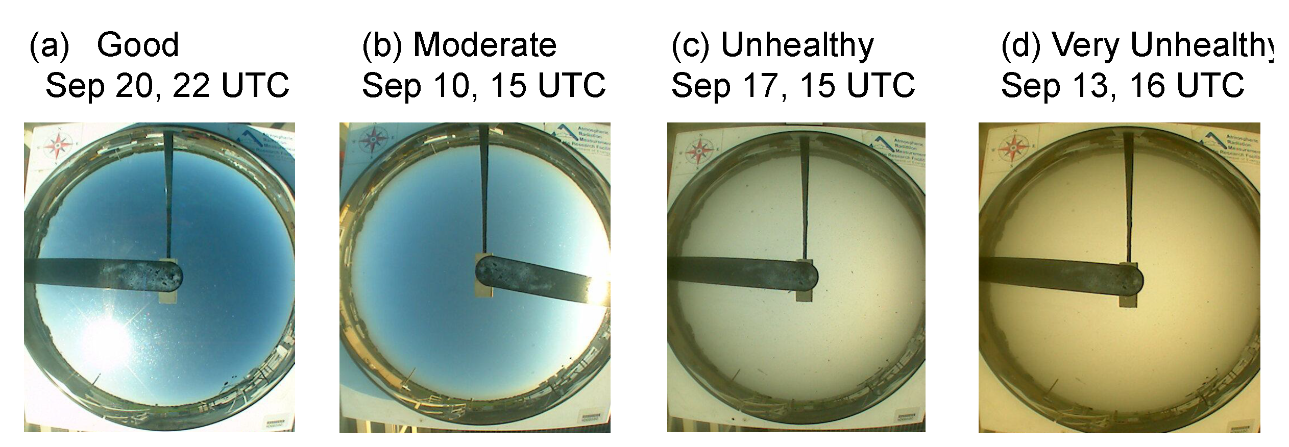
Figure 2.
Training progression of the MobileNetv2 model with transfer learning : (a) Training and validation accuracy increase with number of epochs used for training. (b) Training and validation losses both decrease with number of epochs used for training.
Figure 2.
Training progression of the MobileNetv2 model with transfer learning : (a) Training and validation accuracy increase with number of epochs used for training. (b) Training and validation losses both decrease with number of epochs used for training.
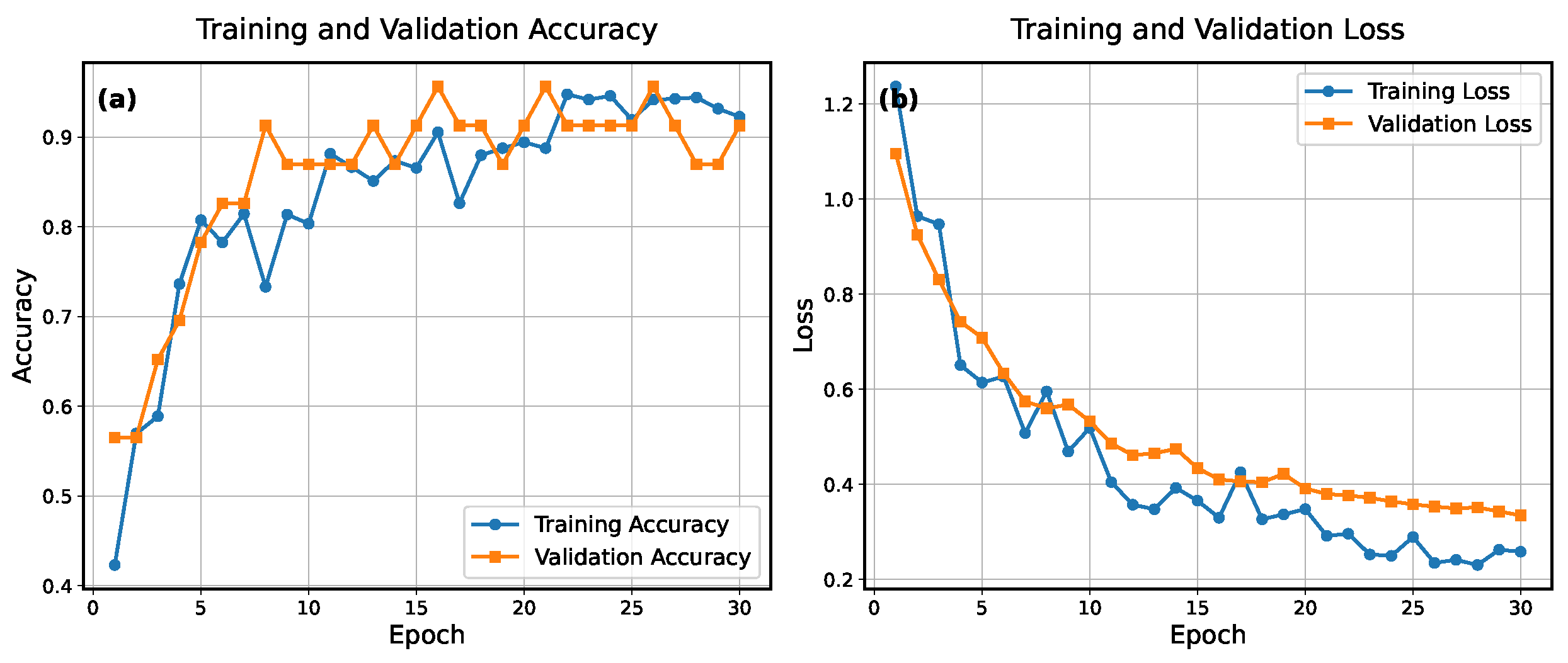
Figure 3.
Model predicted softmax probabilities (Y-axis) represented by 4 grouped colored vertical bars for different AQI classes wherein the tallest bar for each image represents the maximum probability that a given test image belongs to a certain AQI class. Images shown on X-axis from left to right are selected at random from the validation data during Sep 2020 from each of the 4 AQI classes (ground truth) showing that the model successfully classifies each image to its respectively known AQI class. The 5th rightmost test image is from August 2018 wildfires classified as "unhealthy" based on PM2.5 concentrations measured during the 2018 wildfires, and was not included in either training or validation datasets (image previously unseen by the model).
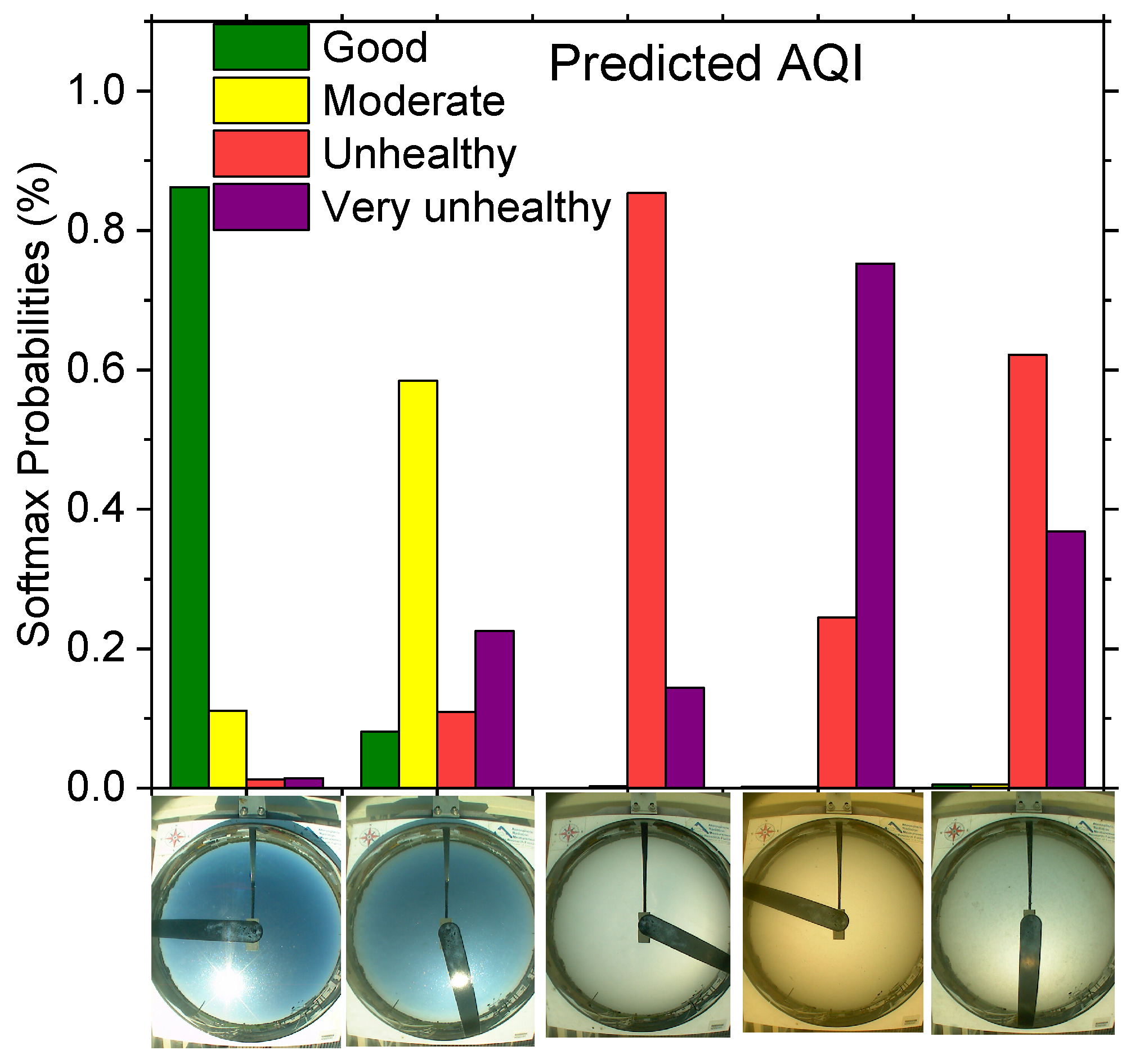
Figure 4.
Central estimates of the relative health risk from exposure to wildfire smoke determined from local PM2.5 measurements using integrated exposure response functional graphs that relate the different causes of death to outdoor and indoor air pollution and smoking [8]. A relative risk of 1 corresponds to PM2.5 concentrations of 0-2.4 .
Disclaimer/Publisher’s Note: The statements, opinions and data contained in all publications are solely those of the individual author(s) and contributor(s) and not of MDPI and/or the editor(s). MDPI and/or the editor(s) disclaim responsibility for any injury to people or property resulting from any ideas, methods, instructions or products referred to in the content. |
© 2025 by the authors. Licensee MDPI, Basel, Switzerland. This article is an open access article distributed under the terms and conditions of the Creative Commons Attribution (CC BY) license (http://creativecommons.org/licenses/by/4.0/).
Copyright: This open access article is published under a Creative Commons CC BY 4.0 license, which permit the free download, distribution, and reuse, provided that the author and preprint are cited in any reuse.


