
Submitted:
18 February 2025
Posted:
19 February 2025
You are already at the latest version
Abstract
Due to climate change, forest regions in California, Western Australia, and Saskatchewan, Canada, are increasingly experiencing severe wildfires, with other climate-related issues affecting the rest of the world. Machine learning (ML) and artificial intelligence (AI) models have emerged to predict wildfire hazards and aid mitigation efforts. However, inconsistencies arise in the wildfire prediction modeling domain due to the database adjustments required to enable complex and real-time modeling. To help address this issue, our paper focuses on creating wildfire prediction models through One-class classification algorithms: Support Vector Machine, Isolation Forest, AutoEncoder, Variational AutoEncoder, Deep Support Vector Data Description, and Adversarially Learned Anomaly Detection. Five-fold Cross-Validation was used to validate all One-class ML models to minimize bias in the selection of the training and testing data. These One-class ML models outperformed Two-class ML models using the same ground truth data, with mean accuracy levels between 90 and 99 percent. Shapley values were used to derive the most important features affecting the wildfire prediction model, which is a novel contribution to the field of wildfire prediction. Among the most important factors for models trained on the California data set were the seasonal maximum and mean dew point temperatures. These insights will support mitigation strategies. In providing access to our algorithms, using Python Flask and a web-based tool, the top-performing models were operationalized for deployment as a REST API, with outcomes supporting the potential of our solution for strengthening wildfire mitigation strategies.
Keywords:
One-class Machine Learning Models
; Wildfire Prediction
; Wildfire Prediction Features
; Wildfire Prediction Tool
1. Introduction
Wildfires have emerged as a critical global concern, annually destroying vast forested areas and significantly impacting the environment, economy, and public health [1,2]. The natural causes of wildfires include lightning strikes, volcanic eruptions, dry climates, and dense vegetation [3]. However, studies indicate that human activities—such as unattended campfires, discarded cigarettes, and intentional acts of arson—are responsible for nearly 85–90% of wildfire occurrences [3]. This alarming trend underscores the need for continuous monitoring and, more importantly, predictive capabilities to forecast the likelihood of widespread and intense wildfires. Such foresight allows fire management authorities to take timely actions to effectively mitigate damage [4,5].
Machine learning (ML) and artificial intelligence (AI) methods offer promising tools for developing predictive wildfire models [4]. For example, the European Centre for Medium-Range Weather Forecasts has developed the Probability of Fire (PoF) tool, which employs ML techniques to forecast fire occurrences globally with high resolution, up to ten days in advance [5]. Nevertheless, several challenges hinder the effectiveness of these models, including technical limitations, environmental complexities, and the difficulty in identifying specific factors that contribute to wildfire ignition. Variations in atmospheric conditions—such as air temperature, relative humidity, wind speed and direction, and spatiotemporal dynamics—further complicate these predictions [2,6]. Another significant challenge is the infrequent and irregular occurrence of wildfires, which makes it difficult to acquire balanced datasets for training models that can distinguish wildfire from non-wildfire events [7].
To address this issue, one-class classification approaches are explored. These methods are particularly effective for anomaly detection tasks where only positive class data is available, such as in predicting rare events or fraud detection [7,8]. Common algorithms include One-Class SVM, Isolation Forest, and Autoencoders. In contrast, two-class (binary) classification is designed for datasets with two labeled categories, aiming to differentiate between them—this is useful in applications like spam filtering or disease diagnosis [9]. While binary classification performs well for balanced datasets, one-class classification is better suited for scenarios with limited class variety, which influences the selection of appropriate models and evaluation metrics [7].
Despite advancements, few wildfire prediction models progress to deployment, limiting their practical applications [4,10]. Integrating ML models into Application Programming Interfaces (APIs) to create user-friendly tools represents an opportunity to enhance the utility of wildfire prediction systems. This study aims to address this gap and contributes in the following ways:
- A comparative evaluation of one-class classification algorithms and two-class models is conducted to determine their suitability for predicting wildfire risk using two fire incidence datasets.
- Shapley values [11] are used to interpret feature importance within one-class ML models, providing explainability and insights into the factors influencing wildfire predictions.
- A novel architecture for a web-based wildfire prediction tool is proposed, operationalizing the best-performing one-class ML model via a REST API.
The study focuses on California and Western Australia as contexts for wildfire probability prediction. California, a high-risk wildfire zone in the United States, recorded 4.2 million acres burned in a single year, resulting in 31 human fatalities [1]. Similarly, the 2019–2020 Australian wildfires devastated 17 million acres, causing the loss of three billion animals. New South Wales and the Australian Capital Territory accounted for 31.6 million acres burned, while Western Australia ranked second with approximately 5.4 million acres lost [12,13].
This work’s objective is to assess the performance of one-class ML algorithms in predicting wildfire risk using historical fire data from California (2012–2016) and Western Australia (2000–2020). By focusing on these regions, this study aims to provide insights into the efficacy of one-class models in overcoming the challenges of wildfire risk prediction and enhancing mitigation strategies.
The rest of the paper is organized as follows. In Sect.Section 2 we provide the study background and describe the One-class ML algorithms used in our experiments. Next, in Sect. Section 3 we describe the data set for the Californian and Western Australian case studies. Our methodology is then provided in Sect. Section 4, and the results of applying our methodology are presented in Sect. Section 5. In Sect. Section 6, the deployment of the ML models is discussed, followed by the web-based prototype evaluation in Sect. Section 7. Finally, in Sect. Section 8 we identify the threats to validity and limitations of our study ending with Sect. Section 9 where we summarise our findings and outline opportunities for future work.
2. Background
Defining a negative sample dataset for complex events such as wildfires presents significant challenges. Numerous non-fire data points could be incorrectly labeled without proper validation for a specific location, date, and time. This issue can be addressed using a One-class classification model, which establishes a class boundary based solely on positive data labels [4,8,10].
In One-class classification, the model assigns a data point as an inlier (•) if its probability exceeds the chosen threshold. Conversely, if the probability is below the threshold, the data point is classified as an outlier (?), as illustrated in Figure 1(a). The selection of an accurate threshold is crucial to ensure the correct classification of inliers and outliers. Typically, the classification boundary in One-class learning is designed to accept most positive data labels while rejecting only a minimal number of outliers, as shown in Figure 1(b). During training, the model relies exclusively on positive data labels, treating outliers as negative labels or non-fire events [7,8].
This approach has effectively tackled problems such as anomaly detection, outlier identification, and concept-based learning, particularly in cases where labeled negative samples are scarce or unreliable [9]. It provides a robust framework for learning from positive data while mitigating the risk of incorrectly labeling complex events like wildfires.
As noted above, the model’s outcome probabilities, as well as its inlier and outlier predictions, are affected by the threshold value. When the threshold is greater than a certain value for a given prediction instance [12,14][p. 159], it will be detected as a fire (inlier). For our experiments, each One-class ML algorithm’s functionality is described below.
In terms of our approaches, the Support Vector Machine (SVM) is a supervised learning model that analyses data and identifies patterns for both classification and regression tasks [15]. The One-class variant refers to two types of One-class SVM (OCSVM). The standard OCSVM uses a sphere of minimal volume to contain a specified proportion of training instances [16]. The other OCSVM trains objects using a hyperplane in a kernel feature space. Data is transformed to a higher dimensional space in order to investigate the possibility of constructing a hyperplane decision boundary, with the assumption that all training points belong to one class and all non-training points belong to another. To generate the ML model in the experiments, the latter OCSVM algorithm was used. The One-class OCSVM operates in such a way that standard data clustered into a single region has a high density, while outliers are detected as low-density regions. New data points can be tested based on density regions to detect normal or outlier cases.
Isolation Forest (IF) is a binary random forest approach in which each node randomly chooses a dimension, and then a splitting threshold [17]. It will keep going until each node has a single sample. This method is used to build an ensemble of trees. A sample with exceptional values has a higher chance of being isolated early in the growth of the tree by chance than samples in clusters; as a result, the average depth of samples in the ensemble of trees directly affects the abnormality score [17].
A recent overview of ML and AI algorithms used in wildfire prediction are summarised in [18] which discussed models that are based on Artificial Neural Networks (ANN) including ones based on Radial Basis Function ANNs [19]. For our experiments we similarly adopted an AutoEncoder (AE) which is a type of multi-layer ANN for unsupervised learning that copies input values to output values, allowing mapping from high-dimensional space to lower-dimensional representation [20]. To reduce reconstruction errors, input data is encoded in the hidden layers. This method forces the hidden layers to learn the most patterns in the data while ignoring the “noise”. Anomalies are defined as input data with a high reconstruction error. In contrast to an AE, the Variational AutoEncoder (VAE) learns the parameters of a probability distribution representing the data, which could make the model more adept at spotting anomalies [20].
Like AE and VAE, the goal of DeepSVDD [21] is to learn network parameters collaboratively while minimising the average distance from all data representations to the center for this algorithm. Normal data are closely mapped to the center for this algorithm, whereas anomalous data are mapped farther from the centre or outside a hypersphere [22]. In DeepSVDD, ANN are used as One-class classifiers, where any data points which the neural network rejects is categorised as an outlier. Network weights are derived from the training data. These trained network weights are then used in the process of testing new data instances. We have selected DeepSVDD [21] and ALAD [23] due to their popularity in performing prediction domains.
Finally, ALAD [23] is a reconstruction-based anomaly detection technique that assesses how well a sample is reconstructed by a Generative Adversarial Network (GAN). GANs are adopted as they can model complex high-dimensional distributions of real-world data, implying that they could be useful in anomaly detection. ALAD is a promising approach in complex, high-dimensional data. ALAD is based on bidirectional GANs and contains an encoder network that maps data samples to latent variables. During training, this learns an encoder from the data space to the latent space, making it significantly more efficient at test time. ALAD assesses how far a sample is from its reconstruction by the GAN, where normal samples should be accurately reconstructed while anomalous samples are likely to be poorly reconstructed.
3. Data set
The work performs three case studies. The first case study is based on California in the United States of America, which spans a land area of 423,970 square km1. From 2012 to 2016, 7,335 wildfire events were recorded in California by US Federal land management agencies, NOAA, the American Scientific Agency, MODIS 500m resolution satellite images, and the US Census Bureau. The variables for the Californian data set were acquired from these agencies, and are listed in Table 1. The collected data were combined into a data set that was geolocated and transformed into an appropriate format for further analysis.
For the second case study for Western Australia, the ground truth data source was the Department of Biodiversity, Conservation, and Attractions2, from which 33,300 wildfire incidents spanning from 2001 to 2020 were collected. Weather data pertaining to the wildfire locations were sourced from the same department.
Additionally, live fuel moisture content data were similarly procured from MODIS 500m resolution satellite images for the closest wildfire event, while social data including the latest population figures for the years 2001 to 2020 were obtained from the Australian Bureau of Statistics. All the features used for this case study are listed in Table 2.
Although the majority of the features from for case study and one and three data sets were constructed were the same, there were differences in features representing vapor pressure readings. For the Californian data set, there was a minimum vapor pressure (VPDMIN_hpa) and maximum vapor pressure (VPDMAX_hpa) for a fire incident. In contrast, the Western Australian data set contained a reading of the vapor pressure at 9AM (VPD9AM_hpa) and at 3PM (VPD3PM_hpa) on the day of the fire incident.
Data pre-processing steps involved eliminating noisy data that contained errors, imputing missing data, converting categorical data to numerical data, handling outliers, and scaling the data. More specifically, for both data sets the Mean_Sea_Level_Pressure, Mean_Station_Pressure, Mean_Wind_Speed, and Maximum_Sustained_Wind_Speed features which corresponded to historical fire locations Universal Kriging-based interpolation [33] were used to interpolate the values for these weather parameters. All categorical variables were converted into numerical variables using the Python’s scikit-learn package’s LabelEncoder pre-processing function to produce valid numerical values for subsequent input to the ML algorithms as recommended by [34] since the ML algorithms adopted in this work all accept only numerical values.
Finally, as the features contained different ranges of values, data scaling was used to normalize the data set to enable comparisons between features. Again, the Python scikit-learn package was used and the StandardScaler module was used to transform and scale the data to zero mean and unit variance with a view to enhance the ML models’ generalizationability to the testing data.
4. Methodology
As demonstrated in Figure 2, developing a decision support system for wildfire prediction involves a number of steps, including data preparation, processing, modelling, validation of ML models, and the potential for deployment of ML models.
Wildfire features, weather features, Live Fuel Moisture Content (LFMC) features, and social features are the four input categories that are used. The data set was encoded and scaled to test the ML models based on One-class classification. Below is a more thorough explanation of these steps.
The relevant classifier function calls were used during model training to fit the model to the data. Hyper-parameter tuning was used to configure the function’s hyper-parameters, eventually producing one ML model for each classifier type that performed the best. During the tuning process, the hyper-parameters of the models were adjusted to achieve the best accuracy based on the most significant features determined by the ML algorithm. This procedure used the Python hyperopt package [35].
To elaborate, the first step was to specify relevant hyper-parameters for the ML models with predefined options and a range of values. The ML models were then trained for 80 iterations using various combinations of those hyper-parameters. Within each iteration, each model was trained using Five-Fold Cross Validation (CV), and the average performance of the model was used to tune the hyper-parameters for the following model. Target values were predicted using testing data and then on the entire data set using the best-performing ML model via 20 times Five-Fold CV. This process produced mean Accuracy, Precision, Recall, and F1-Score classification metrics.
5. Results
5.1. One-class Machine Learning Model Results
Table 3 summarises the performance of the One-class ML models for the Californian data set. The number of inliers (fire positive) predictions, which correspond to the number of actual wildfire events, and the number of outliers (fire negative) predictions are used to assess the effectiveness of the applied ML approaches. The results from Table 3 highlight that the OCSVM (PyOD) model was the best performing One-class classifier, achieving a mean test Accuracy of 0.99, mean Precision of 1.00, mean Recall of 0.99, and mean F1-Score of 0.99. A more objective assessment of the OCSVM (PyOD) model through 20 × Five-Fold CV resulted in its performance being higher than the other ML models observed.
With mean test Accuracy of 0.99, Precision of 1.00, Recall of 0.99, and F1-Score of 1.00, the IF model produced results comparable with the other ML models validating its outstanding performance. Mean test Accuracy, Precision, Recall, and F1-Score for the AE and VAE models ranged from 0.99 to 1.00. Additionally, the mean test Accuracy, Precision, Recall, and F1-Score values for the DeepSVDD and ALAD ML models were lower ranging from 0.87 to 1.00. It should be noted that both OCSVM ML models, despite being less complex than an ALAD and DeepSVDD model, perform better on all mean test metrics providing adequate support for the outcomes of adopting simpler One-class ML models.
Compared with the results documented in Table 3, the performance of the ML models presented in Table 4 revealed that the OCSVM (PyOD) model clearly exhibited consistently high results across all the model evaluation metrics apart from when tested using 20 × Five-Fold CV. However, the better ML model that obtained the highest performance using this criterion was the OCSVM (sklearn) model. These results might in part be due to the increased size of the Western Australian data set and the reduced number of outliers that the OCSVM (PyOD) algorithms was required to detect compared with the number of outliers the OCSVM (sklearn) model was required to detect. This finding aside, the overall results from Table 4 indicate the One-class models still achieved a mean test Accuracy of 0.99, mean Precision of 1.00, mean Recall of 0.99, and mean F1-Score of 0.99.
5.2. Two-Class Machine Learning Outcomes for the Same Ground-Truth Data
We assess the One-class ML approach using the same ground truth data and a randomly generated equal amount of false data [36], created by applying Two-class ML models for the California regions. Sayad [37] used a similar approach in representing negative samples using random timestamps and locations. Hence, the same approach was followed in creating a false data set. Furthermore, commonly used wildfire prediction models using Two-class ML models were investigated and chosen for this use case. As shown in Table 5, the Two-class ML algorithms were used with supporting literature for predicting wildfires.
The outcome shows that similar Two-class-based ML models achieved mean test Accuracies from 0.63 to 0.68 for the test data set. Mean test Precision recorded values from 0.65 to 0.66 and average mean Recall values ranged from 0.73 to 0.76. Mean test F1-Score values recorded a range from 0.69 to 0.72. Hence, these results suggest that the Two-class models exhibit reduced performance for the selected data sets compared to One-class ML models using the same ground truth data. Therefore, One-class ML models can serve as good alternatives in prediction models such as wildfire risk, which has limited ground truth data over the period in question.
5.3. Feature Importance Derived Using Shapley Values
This section examines the results obtained through the application of Shapley values, which emphasize the most crucial features and their impact on One-class ML models. These values are obtained by using game theory principles and coefficients from the internal linear regression [11].
The Shapley value is a metric used to determine the average marginal contribution of each feature when considering all possible combinations (coalitions) of features [11]. For example, to calculate the Shapley value of the mean wind speed, one needs to evaluate all possible coalitions of features that include or exclude the mean wind speed. For each coalition, the marginal contribution of the mean wind speed to the target variable (e.g., ignition probability) is assessed. By aggregating these marginal contributions across all coalitions, the mean marginal contribution of the mean wind speed is obtained, which represents its Shapley value.
Using Shapley values [11], features on the Shapley plots are arranged in descending order of importance so the feature at the top of the Shapley plot is the most important feature for predicting that activity (class). Dots on the Shapley plots correspond to an instance from the data set. The color of the dot ranges from a low value (blue) or a high value (red). The position of the dot on the x-axis shows whether the feature for that data instance has a positive impact (to the right) or a negative impact (to the left) on the model’s prediction of a class as measured by the Shapley value for that feature. The plot on the left in Figure 3 shows the average impact of the features on the One-class OCSVM (PyOD) ML model’s outputs for California.
Based on Figure 3 the most influential attributes include the maximum and average dew point temperatures associated with different seasons. Then Mean_Sea_Level_Pressure, PPT_mm, and lfmc_mean are the second set of essential features that influence wildfire prediction. For example, the temperature variables and lfmc_mean have a more significant impact on the model output for the risk of wildfire than does the population. Also, high LFMC is more susceptible to ignition and can signal more fire spread [28]. Mean_Sea_Level_Pressure is the average level of one or more bodies of water on Earth from which elevation can be calculated. With increasing elevation, sea level pressure decreases. Wind speed and direction are both factors in the wind effect. The dry wind is one of the primary causes of wildfire spreading. The rate of wildfire spread has been estimated to be around 8% of wind speed, regardless of fuel type, especially in dry fuel moisture conditions [4].
Similar trends were found when investigating the importance of the Shapley values obtained from four of the remaining six ML models as shown in Table 6. The percentage value in each column of the table quantified the contribution of that feature for predicting a wildfire as measured by the Shapley value for that feature. For example, with the One-class SVM (PyOD) the contribution of TMAX_c to the prediction of a wildfire incident was 11.30% but for the same ML model Population had only a negligible contribution of 0.52%. Conversely for the Variational AutoEncoder the contribution of PPT_mm was 45.40% which suggests that this feature has significant importance to VAE model prediction whereas the Shapley value for Mean_Sea_Level_Pressure contributed only 0.28%, indicating this feature had much lower importance for this model.
In conclusion the results from Table 6 indicate that the features which have high percentage values for each ML model should be given more importance in the modelling process. Confirmation of how the features which significantly influence other ML models’ outcomes should also be investigated as demonstrated by the results of the Shapley value plot is presented in Figure 3.
6. Deployment of Machine Learning Models
The results from testing the features and models informed a web-based tool, which is presented in the following section to showcase the efficiency and practicality of One-class ML models. The web-based tool3 is presented as a contribution to the state-of-the-art ML-based wildfire prediction domain (see Figure 4). The main objective of this phase of research is to deploy the results of the selected ML model using a REST API, which will then be fed into a web-based tool. The web-based tool’s goal is to provide long-term wildfire predictions based on One-class classification-based ML models that can predict the start of a wildfire one week in advance for any given location in California. This can also help international wildfire management authorities test wildfire prediction models across multiple geographies. The web-based tool is also useful for countries that do not have access to wildfire forecasting systems. However, this is not meant to replace current regional wildfire forecasting systems.
The ML model is fed with 20 features (see Sect. Section 3) from four categories and six probability rates of danger levels, which are mapped by the decision scores (d) of the One-class ML models: No Danger (d ≤ 0), Low (0 < d ≤ 60), Moderate (60 < d ≤ 80), High (80 < d ≤ 90), Very High (90 < d ≤ 97) and Severe (97 < d ≤ 100). The fire danger rating breakpoints used are similar to fire spread probabilities modelled by the US Wildland Fire Decision Support System [44] to create these threshold classes. The selection of these fire danger rating class thresholds was informed by historical fire danger outcomes, as documented in [45]. The Flask REST service for the web-based tool uses three other external REST APIs for generating wildfire prediction outcomes:
- The publicly available free Open Topo Data elevation REST API which gives elevation data of any location when latitude and longitude are given.
- The OpenWeather REST API provides historical, current and forecasted weather details through REST APIs for any point on the world.
- USGS Earth Explorer Website hosts LFMC data as different vegetation indexes carry a file format of all locations of California based on a MODIS grid.
The four main functionalities listed below were thus identified as the outcome of this web-based tool:
- Choose some historical wildfire events to train the ML models and validate the model output. Users can also alter the input parameters and analyse and explore the most important features of the ML models.
- Select any location in California and Western Australia using the map, manually enter the input features, and use a probability to predict wildfire susceptibility.
- Search all input features for the next seven days.
- View historical yearly wildfire heat-maps based on ML model training and testing data.
Several technological advancements in the field of wildfires have emerged in recent years as a result of the high costs and practical difficulties of fighting wildfires. Technology training is at the top of the list because it is crucial for sharing common resources and standards for information on fire danger and communication between fire authorities. The use of technological systems to forecast and predict the occurrence of wildfires has enabled emergency response teams to plan ahead and take preventative action. Firefighters must receive the necessary training to deal with such emergencies. Implementing a straightforward, inexpensive prototype can significantly lower the price of intricate training. Large financial budgets can also be set aside for public education campaigns about wildfire prevention and natural wildfire occurrences. The infrastructure cost of the Google Cloud Platform (GCP) (virtual machine and domain name) constitutes the sole cost element for the implementation of this web-based tool. The remaining programs and services are either open source, free, or have a free usage tier. Hosting this in an on-premise local area network may thus result in an infrastructure cost saving in terms of infrastructure. The web-based tool has a monthly fee of $42 New Zealand Dollars (NZD) and can forecast wildfires up to a week in advance4. This tool can handle up to 1000 predictions daily, each forecast extending up to seven days ahead. It can process a maximum of five requests per second on the web platform. Considering its cost and functionalities, our deployed solution presents a budget-friendly choice for new researchers to test their wildfire prediction models. Moreover, these solutions are adaptable for different areas and offer fire authorities a chance to test them for public use at a reasonable price. To assess the utility of this tool, a user-based questionnaire evaluation has been carried out, the results of which are reported in the next section.
7. Web-Based Prototype Evaluation
Users have access to wildfire prediction capabilities through the website www.bushfirepredict.com. This online tool facilitates fire predictions in California and Western Australia for any specified location within these regions. Users can select locations from a heatmap to forecast wildfires up to one week in advance. Furthermore, historical wildfire events can be examined using specific past incidents. ML models are utilized to generate prediction results, offering both manual and automatic search options. Predictions are displayed with positive or negative labels indicating potential wildfire occurrences or the absence thereof. Additionally, potential wildfires are categorized into fire danger rating classes, ranging from No Danger to Severe levels.
The utility of the web-based tool was assessed by administering an 18-question questionnaire to New Zealand computing practitioners covering general design, performance, and content. The questionnaire was completed in an average of 15 minutes by 11 participants. More than 81 percent of respondents used Chrome, while Firefox was also used by some, according to the findings. Additionally, over 63% of respondents reported feeling extremely satisfied, with the remaining respondents rating their satisfaction as “somewhat”. Experience with the mobile phone view using different browsers produced mixed results, with the majority of respondents being satisfied, 18% being neither satisfied nor dissatisfied, and the remaining 9% being extremely dissatisfied. The mobile phone version needs to be enhanced further as a result. The overall design of the tool resulted in an above-average ranking for all feedback. Performance-wise, the speed of information retrieval from the input feature fields, the speed of ML prediction, and the response time were all very quick. Additionally, the overall performance was rated as being better than satisfactory, with 80% stating that it performed excellently and with positive feedback exceeding 63% for the tool’s content when measuring the understandability of input and output features of the accuracy of wildfire prediction outcomes. This results in a high-performance rating for the web-based tool5.
8. Threats to Validity and Limitations
We acknowledge that there are some uncontrolled factors that might have impacted the results reported in our study. For example, the One-class ML models demonstrated high prediction accuracy for the states of California and Western Australian instead of scaling these ML models to countrywide analyses. In doing so we highlighted the need for region-specific modeling due to varying climate and vegetation factors. This issue necessitates frequent recalibration of the ML models to address these environmental changes. By doing this, the efficacy and reliability of these ML models to predict wildfires would be maintained.
Next, accurate climate forecasting is critical for predicting wildfires, but climate change complicates this, limiting the ML models’ effectiveness. To mitigate this issue we took steps to source appropriate climate data informed by relevant prior research to generate the data sets. In the future it is expected that data produced by more recent climate forecasting models would mitigate this problem.
Furthermore, location-specific granular data was interpolated from station-based weather data, though the inclusion of more specific location-based data acquired from hand-held sensors or wireless sensor networks might improve model accuracy. The adoption of higher resolution satellite or drone-based images could also enhance LFMC values but potentially incur a higher financial cost to obtain.
Another threat was that the ML models constructed could be subject to over-fitting. Our methodology accounted for this potential risk by adopting Five-Fold CV when establishing the best hyper-parameters for a specific One-Class ML model type. A thorough assessment of the best One-Class ML model performance was then conducted using 20 times Five-Fold CV. In both cases the objective of using CV was to reduce the risk of over-fitting and increase the ability for the ML model to generalise to unseen data.
Finally, the One-class and Two-Class ML models, were built using currently available Python libraries implementing existing One-Class and Two-Class learning algorithms. The reliance on using these Python libraries not only limited the scope of applying other appropriate ML algorithms for the purpose of wildfire prediction but also did not consider non ML-based approaches. Wildfire prediction using physical models [46] or statistical models [47] might yield slightly different results with the same dataset, pointing to a limitation in using ML for wildfire prediction. Despite this, our methodology was consistently applied across different geographic locations supporting model re-usability. Future testing of our methodology in diverse environmental and geographical contexts can further validate our research approach.
9. Conclusion and Future Work
In summary, historical wildfire events in California and Western Australia were represented using a total of 20 features. Seven different One-class ML algorithms were used in order to train multiple models. After the hyper-parameters of the ML models were tuned, the models were validated using repeated 20 × Five-Fold CV. The average test Accuracy of each ML model ranged from 0.90 to 1.00, demonstrating the ML models’ high generic performance for both the California and Western Australian data sets. In addition, Precision, Recall, and F1-Score values were used to evaluate the effectiveness of the ML models.
Not only does our study address the need to create ML-based wildfire prediction models, but, more importantly, it identifies key features from these models that could influence wildfire ignition. As well as our findings being consistent with the outcomes of previous research, we also showed the degree to which these identified features contribute to the risk of a wildfire event.
Finally, we described the development of a web-based prototype that integrates the best performing ML algorithms to model the sequence of wildfire events for wildfire occurrence mapping. The intended audiences for this tool are the general public and wildfire authorities.
The enhanced OCSVM model was added to the tool using the Flask API, and it was inexpensively (with room for future scaling needs) deployed on a web server. This might be distinct from other research areas with distinct traits and ML approaches, though, which will be examined in subsequent work to address such limitations. In addition, the web-based tool’s usability was evaluated to determine its utility.
However, as we only used two data sets for this study, future work will involve the creation of more wildfire data sets from other countries, potentially using different features. Top-ranked features extracted from these ML models using Shapley values may be compared and contrasted with the findings from our existing work to show how the contribution of different features influence the risk of wildfire depending on the location. Similarly, quantifying which hyper-parameters are more important for producing high-performing ML models is a topic for investigation especially as recent work by [48] proposed a more computationally efficient method for this task.
In terms of other future work, we will explore extending the web-based prototype with the integrating of other approaches (e.g., LLM) to model the sequence of wildfire events for wildfire occurrence mapping. The intended audience for this tool will be for both the public and various wildfire authorities. Such an application could contribute to the current methods for early detection of wildfires to mitigate this global problem.
Abbreviations
The following abbreviations are used in this manuscript:
| ML | Machine Learning |
| API | Application Programming Interface |
| AI | Artificial Intelligence |
| SVM | Support Vector Machine |
| IF | Isolation Forest |
| AE | AutoEncoder |
| VAE | Variational AutoEncoder |
| DeepSVD | Deep Support Vector Data Description |
| ALAD | Adversarially Learned Anomaly Detection |
| CV | Cross-Validation |
| OCSVM | One Class Support Vector Machine |
| ANN | Artificial Neural Networks |
| NOAA | National Oceanic and Atmospheric Administration |
| MODIS | Moderate Resolution Imaging Spectroradiometer |
| LFMC | Live Fuel Moisture Content |
| GCP | Google Cloud Platform |
| NZD | New Zealand Dollars |
| LLM | Large Language Model |
References
- Tyukavina, A.; Potapov, P.; Hansen, M.C.; Pickens, A.H.; Stehman, S.V.; Turubanova, S.; Parker, D.; Zalles, V.; Lima, A.; Kommareddy, I.; et al. Global Trends of Forest Loss Due to Fire From 2001 to 2019. Frontiers in Remote Sensing 2022, 3. [Google Scholar] [CrossRef]
- Bowman, D.M.J.S.; Williamson, G.J.; Price, O.F.; Ndalila, M.N.; Bradstock, R.A. Australian forests, megafires and the risk of dwindling carbon stocks. Plant Cell Environ. 2021, 44, 347–355. [Google Scholar] [PubMed]
- Reisen, F.; Duran, S.M.; Flannigan, M.; Elliott, C.; Rideout, K. Wildfire smoke and public health risk. International Journal of Wildland Fire 2015, 24, 1029–1044. [Google Scholar] [CrossRef]
- Jain, P.; Coogan, S.C.; Subramanian, S.G.; Crowley, M.; Taylor, S.; Flannigan, M.D. A review of machine learning applications in wildfire science and management. Environmental Reviews 2020, 28, 478–505. [Google Scholar] [CrossRef]
- European Centre for Medium-Range Weather Forecasts. 2024 was the warmest year on record, Copernicus data show. https://www.ecmwf.int/en/about/media-centre/news/2025/2024-was-warmest-year-record-copernicus-data-show. Accessed: 2025-1-20.
- Miller, C.; Hilton, J.; Sullivan, A.; Prakash, M. SPARK – A Bushfire Spread Prediction Tool. In Proceedings of the Environmental Software Systems. Infrastructures, Services and Applications, Cham; Denzer, R., Argent, R.M., Schimak, G., Hřebíček, J., Eds.; 2015; pp. 262–271. [Google Scholar] [CrossRef]
- Chandola, V.; Banerjee, A.; Kumar, V. Anomaly detection: A survey. ACM Comput. Surv. 2009, 41. [Google Scholar] [CrossRef]
- Khan, S.S.; Madden, M.G. One-Class Classification: Taxonomy of Study and Review of Techniques. The Knowledge Engineering Review 2014, 29, 345–374. [Google Scholar] [CrossRef]
- Nguyen, P.T.; Nguyen, T.T.; Nguyen, N.C.; Le, T.T. Multiclass breast cancer classification using convolutional neural network. In Proceedings of the 2019 International symposium on electrical and electronics engineering (ISEE). IEEE; 2019; pp. 130–134. [Google Scholar]
- Ismail, F.N.; Woodford, B.J.; Licorish, S.A.; Miller, A.D. An assessment of existing wildfire danger indices in comparison to one-class machine learning models. Natural Hazards 2024, 120, 14837–14868. [Google Scholar] [CrossRef]
- Lundberg, S.M.; Lee, S.I. A unified approach to interpreting model predictions. In Proceedings of the Proceedings of the 31st International Conference on Neural Information Processing Systems, Red Hook, NY, USA, 2017; p. 4768–4777. [CrossRef]
- Ismail, F.N. Novel machine learning approaches for wildfire prediction to overcome the drawbacks of equation-based forecasting. PhD dissertation, University of Otago, 2022.
- Ismail, F.N.; Sengupta, A.; Woodford, B.J.; Licorish, S.A. A Comparison of One-Class Versus Two-Class Machine Learning Models for Wildfire Prediction in California. Data Science and Machine Learning. AusDM 2023 2024, pp. 239–253.
- Ismail, F.N.; Amarasoma, S. One-class Classification-Based Machine Learning Model for Estimating the Probability of Wildfire Risk. Procedia Computer Science 2023, 222, 341–352, International Neural Network SocietyWorkshop on Deep Learning Innovations and Applications (INNS DLIA 2023). [Google Scholar] [CrossRef]
- Cortes, C.; Vapnik, V. Support-Vector Networks. Machine learning 1995, 20, 273–297. [Google Scholar] [CrossRef]
- Tax, D.M.; Duin, R.P. Support vector domain description. Pattern recognition letters 1999, 20, 1191–1199. [Google Scholar] [CrossRef]
- Liu, F.T.; Ting, K.M.; Zhou, Z. Isolation Forest. In Proceedings of the 2008 Eighth IEEE International Conference on Data Mining, Piscataway, NJ; 2008; pp. 413–422. [Google Scholar] [CrossRef]
- Alkhatib, R.; Sahwan, W.; Alkhatieb, A.; Schütt, B. A Brief Review of Machine Learning Algorithms in Forest Fires Science. Applied Sciences 2023, 13. [Google Scholar] [CrossRef]
- Ntinopoulos, N.; Sakellariou, S.; Christopoulou, O.; Sfougaris, A. Fusion of Remotely-Sensed Fire-Related Indices for Wildfire Prediction through the Contribution of Artificial Intelligence. Sustainability 2023, 15. [Google Scholar] [CrossRef]
- Patterson, J.; Gibson, A. Deep learning: A practitioner’s approach; O’Reilly Media, Inc.: Sebastopol, CA, 2017. [Google Scholar]
- Ruff, L.; Vandermeulen, R.; Goernitz, N.; Deecke, L.; Siddiqui, S.A.; Binder, A.; Müller, E.; Kloft, M. Deep One-Class Classification. In Proceedings of the Proceedings of the 35th International Conference on Machine Learning; Dy, J.; Krause, A., Eds., 2018, Vol. 80, Proceedings of Machine Learning Research, pp. 4393–4402.
- Kim, S.; Choi, Y.; Lee, M. Deep learning with support vector data description. Neurocomputing 2015, 165, 111–117. [Google Scholar] [CrossRef]
- Zenati, H.; Romain, M.; Foo, C.S.; Lecouat, B.; Chandrasekhar, V. Adversarially learned anomaly detection. In Proceedings of the 2018 IEEE International Conference on Data Mining (ICDM). IEEE Press; 2018; pp. 727–736. [Google Scholar] [CrossRef]
- Pedregosa, F.; Varoquaux, G.; Gramfort, A.; Michel, V.; Thirion, B.; Grisel, O.; Blondel, M.; Prettenhofer, P.; Weiss, R.; Dubourg, V.; et al. Scikit-learn: Machine Learning in Python. Journal of Machine Learning Research 2011, 12, 2825–2830. [Google Scholar] [CrossRef]
- Zhao, Y.; Nasrullah, Z.; Li, Z. PyOD: A Python Toolbox for Scalable Outlier Detection. Journal of Machine Learning Research 2019, 20, 1–7. [Google Scholar]
- Abdollahi, A.; Pradhan, B. Explainable artificial intelligence (XAI) for interpreting the contributing factors feed into the wildfire susceptibility prediction model. Science of The Total Environment 2023, 879, 163004. [Google Scholar] [CrossRef] [PubMed]
- Tonini, M.; D’Andrea, M.; Biondi, G.; Degli Esposti, S.; Trucchia, A.; Fiorucci, P. A Machine Learning-Based Approach for Wildfire Susceptibility Mapping. The Case Study of the Liguria Region in Italy. Geosciences 2020, 10, 105. [Google Scholar] [CrossRef]
- Jaafari, A.; Pourghasemi, H.R. 28 - Factors Influencing Regional-Scale Wildfire Probability in Iran: An Application of Random Forest and Support Vector Machine. In Spatial Modeling in GIS and R for Earth and Environmental Sciences; Pourghasemi, H.R.; Gokceoglu, C., Eds.; 2019; pp. 607–619. [CrossRef]
- Donovan, G.H.; Prestemon, J.P.; Gebert, K. The Effect of Newspaper Coverage and Political Pressure on Wildfire Suppression Costs. Society & Natural Resources 2011, 24, 785–798. [Google Scholar] [CrossRef]
- Jiménez-Ruano, A.; Mimbrero, M.R.; de la Riva Fernández, J. Understanding wildfires in mainland Spain. A comprehensive analysis of fire regime features in a climate-human context. Applied Geography 2017, 89, 100–111. [Google Scholar] [CrossRef]
- Papadopoulos, A.; Paschalidou, A.; Kassomenos, P.; McGregor, G. On the association between synoptic circulation and wildfires in the Eastern Mediterranean. Theoretical and Applied Climatology 2014, 115, 483–501. [Google Scholar] [CrossRef]
- Nunes, A.; Lourenço, L.; Meira Castro, A.C. Exploring spatial patterns and drivers of forest fires in Portugal (1980–2014). Science of The Total Environment 2016, 573, 1190–1202. [Google Scholar] [CrossRef] [PubMed]
- Stein, M.L. Interpolation of Spatial Data: Some Theory for Kriging; Springer Series in Statistics; Springer-Verlag: New York, 1999. [Google Scholar] [CrossRef]
- Tadić, J.M.; Ilić, V.; Biraud, S. Examination of geostatistical and machine-learning techniques as interpolators in anisotropic atmospheric environments. Atmospheric Environment 2015, 111, 28–38. [Google Scholar] [CrossRef]
- Bergstra, J.; Yamins, D.; Cox, D.D. Making a Science of Model Search: Hyperparameter Optimization in Hundreds of Dimensions for Vision Architectures. In Proceedings of the Proceedings of the 30th International Conference on International Conference on Machine Learning - Volume 28, Atlanta, GA, USA, 2013ICML’13, p. I–115–I–123. [CrossRef]
- Tien Bui, D.; Bui, Q.T.; Nguyen, Q.P.; Pradhan, B.; Nampak, H.; Trinh, P.T. A hybrid artificial intelligence approach using GIS-based neural-fuzzy inference system and particle swarm optimization for forest fire susceptibility modeling at a tropical area. Agricultural and Forest Meteorology 2017, 233, 32–44. [Google Scholar] [CrossRef]
- Sayad, Y.O.; Mousannif, H.; Al Moatassime, H. Predictive modeling of wildfires: A new dataset and machine learning approach. Fire Safety Journal 2019, 104, 130–146. [Google Scholar] [CrossRef]
- Nhu, V.H.; Shirzadi, A.; Shahabi, H.; Singh, S.K.; Al-Ansari, N.; Clague, J.J.; Jaafari, A.; Chen, W.; Miraki, S.; Dou, J.; et al. Shallow Landslide Susceptibility Mapping: A Comparison between Logistic Model Tree, Logistic Regression, Naïve Bayes Tree, Artificial Neural Network, and Support Vector Machine Algorithms. International Journal of Environmental Research and Public Health 2020, 17, 2749. [Google Scholar] [CrossRef]
- Ghorbanzadeh, O.; Valizadeh Kamran, K.; Blaschke, T.; Aryal, J.; Naboureh, A.; Einali, J.; Bian, J. Spatial Prediction of Wildfire Susceptibility Using Field Survey GPS Data and Machine Learning Approaches. Fire 2019, 2, 43. [Google Scholar] [CrossRef]
- Michael, Y.; Helman, D.; Glickman, O.; Gabay, D.; Brenner, S.; Lensky, I.M. Forecasting fire risk with machine learning and dynamic information derived from satellite vegetation index time-series. Science of The Total Environment 2021, 764, 142844. [Google Scholar] [CrossRef]
- Goldarag, Y.; Mohammadzadeh, A.; Ardakani, A. Fire Risk Assessment Using Neural Network and Logistic Regression. Journal of the Indian Society of Remote Sensing 2016, 44, 1–10. [Google Scholar] [CrossRef]
- de Bem, P.; de Carvalho Júnior, O.; Matricardi, E.; Guimarães, R.; Gomes, R. Predicting wildfire vulnerability using logistic regression and artificial neural networks: a case study in Brazil. International Journal of Wildland Fire 2018, 28, 35–45. [Google Scholar] [CrossRef]
- Ma, J.; Cheng, J.; Jiang, F.; Gan, V.; Wang, M.; Zhai, C. Real-time detection of wildfire risk caused by powerline vegetation faults using advanced machine learning techniques. Advanced Engineering Informatics 2020, 44, 101070. [Google Scholar] [CrossRef]
- Jolly, W.M.; Freeborn, P.H.; Page, W.G.; Butler, B.W. Severe Fire Danger Index: A Forecastable Metric to Inform Firefighter and Community Wildfire Risk Management. Fire 2019, 2, 47. [Google Scholar] [CrossRef]
- National Interagency Fire Center. National Wildfire Coordinating Group (NWCG). Interagency Standards for Fire and Fire Aviation Operations; Createspace Independent Publishing Platform: Great Basin Cache Supply Office: Boise, ID, USA, 2019. [Google Scholar]
- Sullivan, A.L. Physical Modelling of Wildland Fires. In Encyclopedia of Wildfires and Wildland-Urban Interface (WUI) Fires; Springer International Publishing: Cham, 2019; pp. 1–8. [Google Scholar] [CrossRef]
- Taylor, S.W.; Woolford, D.G.; Dean, C.B.; Martell, D.L. Wildfire Prediction to Inform Fire Management: Statistical Science Challenges. Statistical Science 2013, 28, 586–615. [Google Scholar] [CrossRef]
- Watanabe, S.; Bansal, A.; Hutter, F. PED-ANOVA: Efficiently Quantifying Hyperparameter Importance in Arbitrary Subspaces. In Proceedings of the Proceedings of the Thirty-Second International Joint Conference on Artificial Intelligence, IJCAI-23; Elkind, E., Ed., California, 8 2023; pp. 4389–4396. [CrossRef]
| 1 | |
| 2 | |
| 3 | |
| 4 | More information on the cost calculation can be found on [12]. |
| 5 | More information on the outcome of the questionnaire can be found on [12]. |
Figure 1.
The distinction between One-class classification (a) and Two-class classification (b). Compared with a One-class classification model, a Two-class classification model accepts inlier (positive) data labels but rejects outlier labels.
Figure 1.
The distinction between One-class classification (a) and Two-class classification (b). Compared with a One-class classification model, a Two-class classification model accepts inlier (positive) data labels but rejects outlier labels.
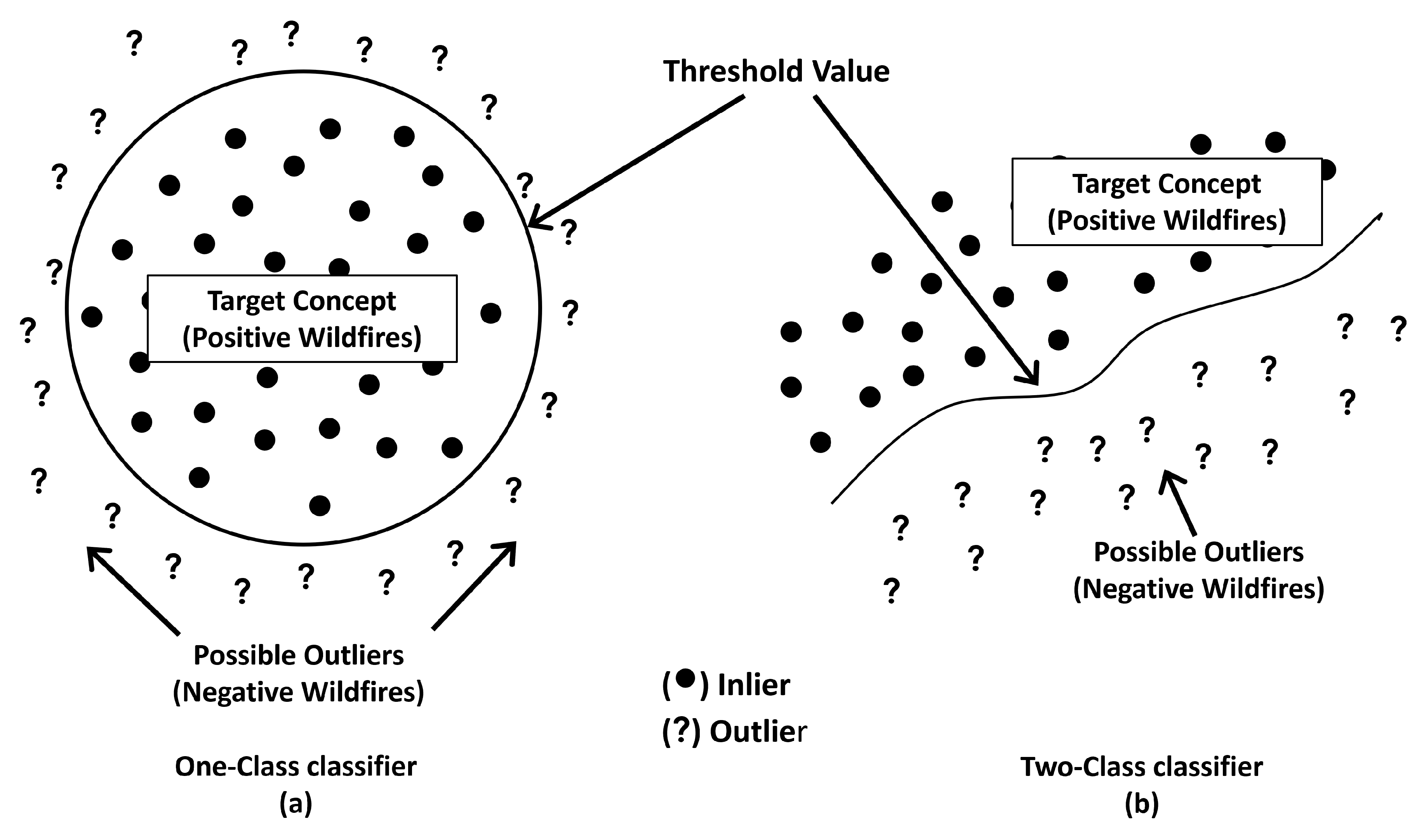
Figure 2.
The process of building a wildfire prediction model involves various steps from data preparation, data pre-processing, model generation using One-class ML, model validation, and deploying ML models through a web-based tool
Figure 2.
The process of building a wildfire prediction model involves various steps from data preparation, data pre-processing, model generation using One-class ML, model validation, and deploying ML models through a web-based tool
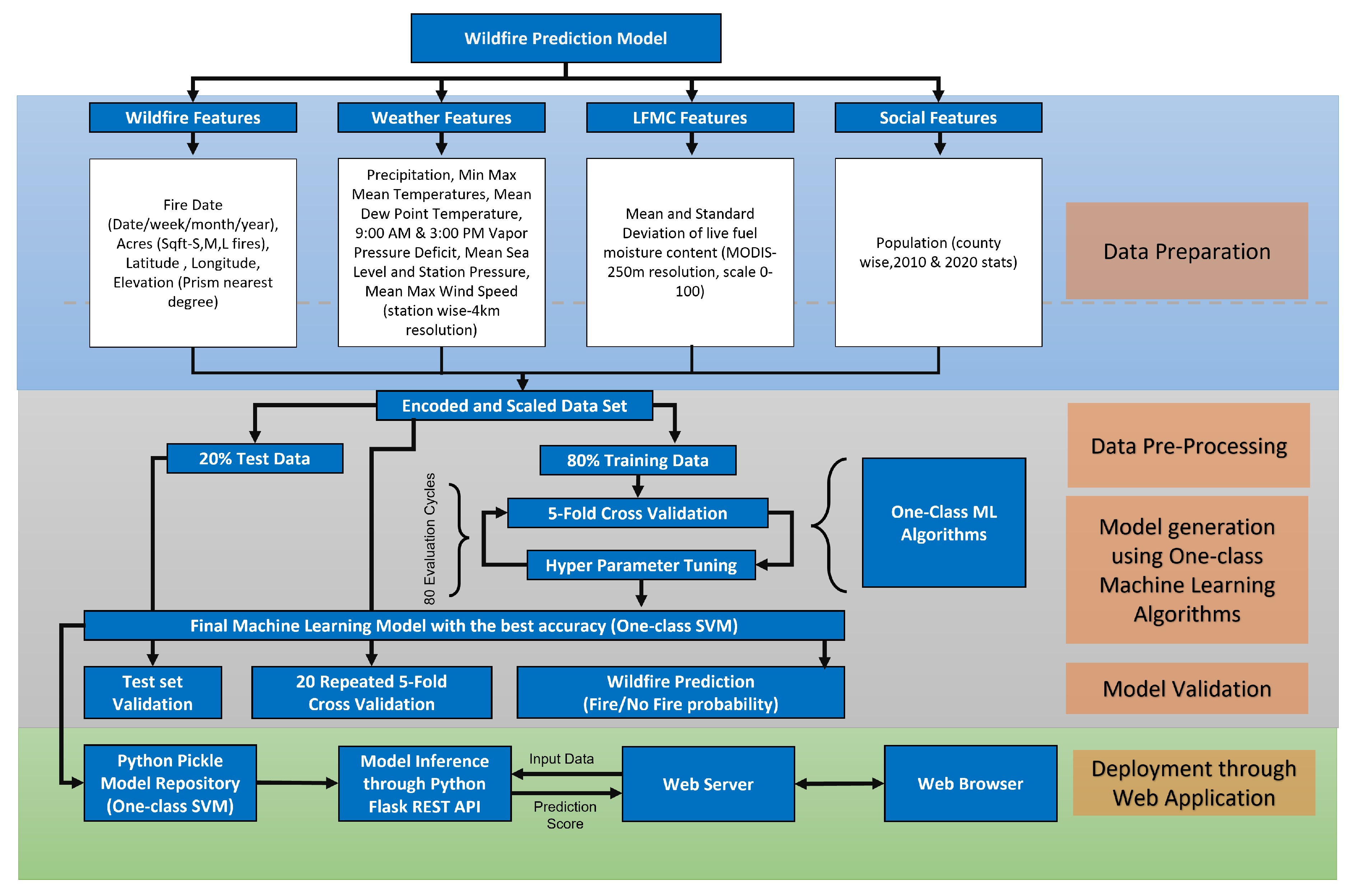
Figure 3.
Shapley values generated from the OCSVM PyOD model (right) shows that the mean and temperature values are high when the model output is predicting positive fire occurrences for California
Figure 3.
Shapley values generated from the OCSVM PyOD model (right) shows that the mean and temperature values are high when the model output is predicting positive fire occurrences for California
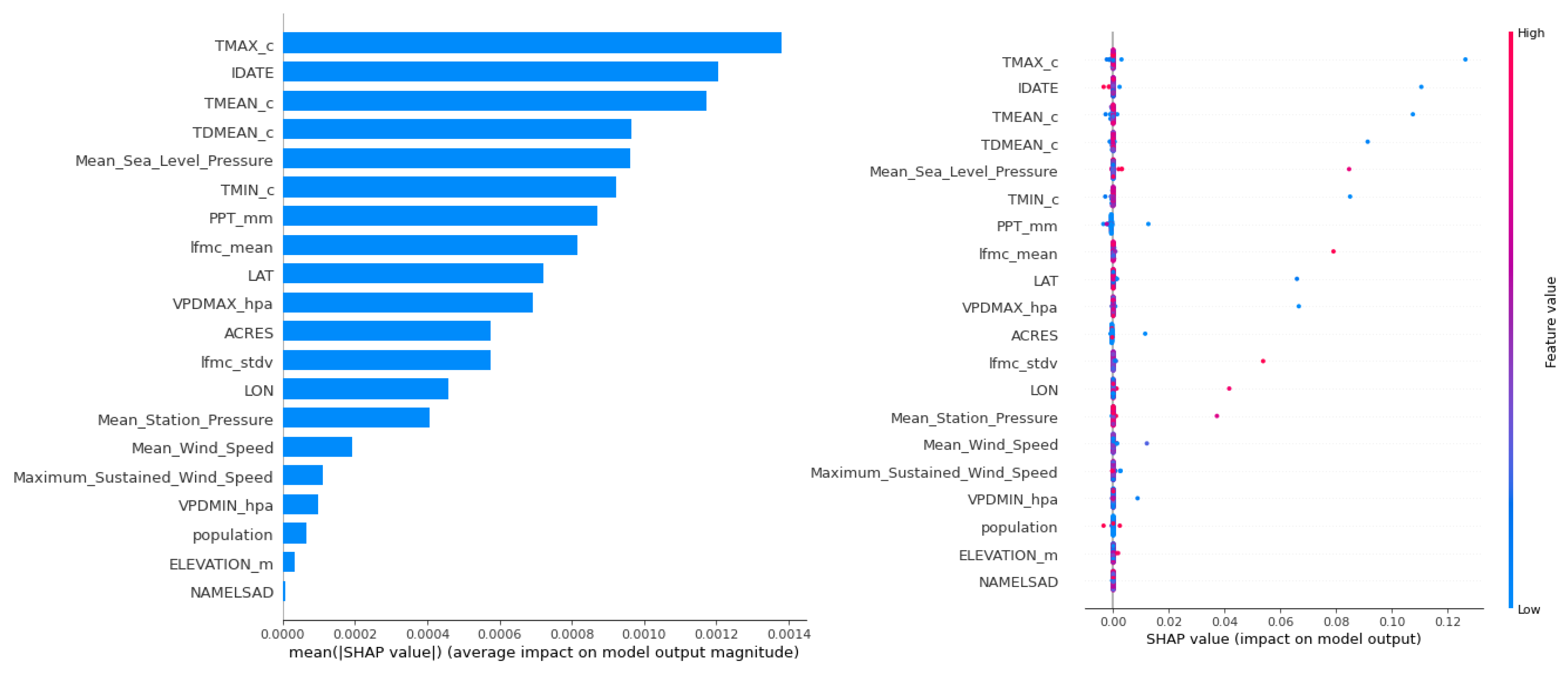
Figure 4.
The deployed ML model’s architecture deriving wildfire prediction outcomes using six fire danger rating levels
Figure 4.
The deployed ML model’s architecture deriving wildfire prediction outcomes using six fire danger rating levels
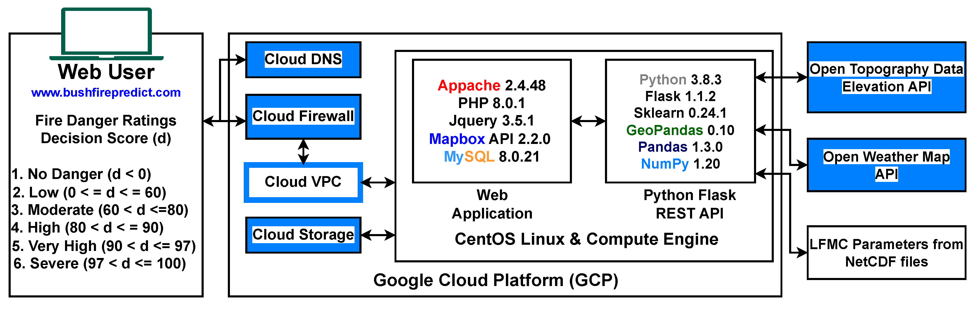
Figure 5.
Inyo 2012-06-30 Fire Event with main input features
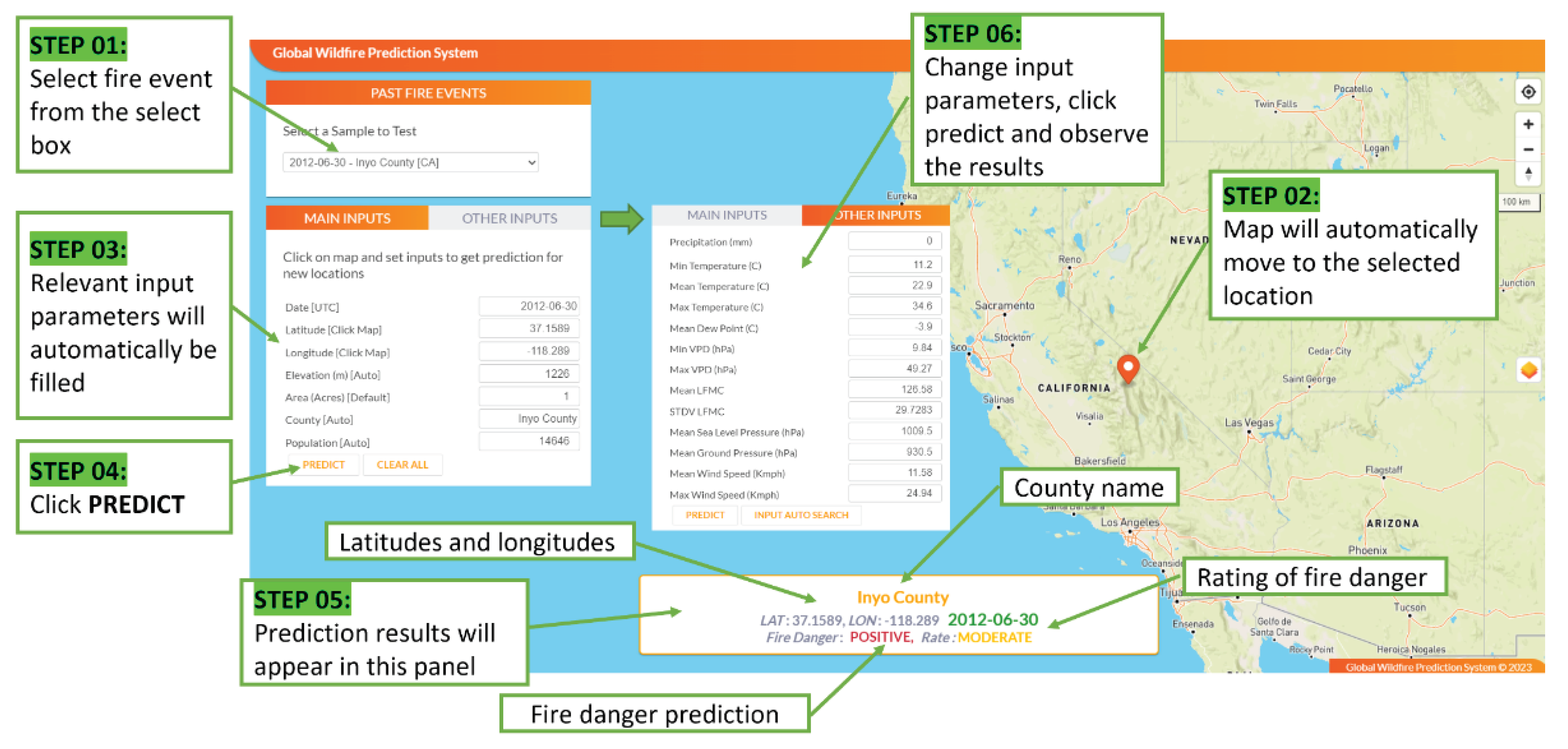

Table 1.
Variables used for ML models - Californian data set (7,335 Events).
| No. | Feature | Description | Prior Research |
|---|---|---|---|
| 1 | IDATE | Fire Occurrence Date (Month & Date as an Integer) | [26] |
| 2 | LAT | Fire location latitude (degrees) | [26,27,28] |
| 3 | LON | Fire location longitude (degrees) | [26,27,28] |
| 4 | ELEVATION_m | Fire location elevation (in meters) | [26,28,29] |
| 5 | ACRES | Acres burnt (in acres) | |
| 6 | PPT_mm | Precipitation (in mm for the fire incident date) | [26,28,30] |
| 7 | TMIN_c | Minimum temperature (in Celsius for the fire incident date) | [28,30] |
| 8 | TMEAN_c | Mean temperature (in Celsius for the fire incident date) | [28,30] |
| 9 | TMAX_c | Maximum temperature (in Celsius for the fire incident date) | [26,28,30] |
| 10 | TDMEAN_c | Mean dew point temperature (in Celsius for the fire incident date) | [28,30] |
| 11 | VPDMIN_hpa | Minimum vapor pressure (in hectopascals) | [29] |
| 12 | VPDMAX_hpa | Maximum vapor pressure (in hectopascals) | [29] |
| 13 | lfmc_mean | Mean fuel moisture for a particular day (numeric) | [28] |
| 14 | lfmc_stdv | Standard deviation of fuel moisture for a particular day (numeric) | [28] |
| 15 | Mean_Sea_Level _Pressure | Mean sea level pressure of the nearest weather station to the wildfire event (in hectopascals) - (Universal Kriging) | [31] |
| 16 | Mean_Station _Pressure | Nearest mean weather station pressure to the wildfire event (in hectopascasl) - (Universal Kriging) | [31] |
| 17 | Mean_Wind_Speed | Mean wind speed for a given location (numeric mph) - (Universal Kriging) | [26,28,29] |
| 18 | Maximum_Sustained _Wind_Speed | Maximum sustained wind speed for a given location (numeric MPH) - (Universal Kriging) | [28,29] |
| 19 | NAMELSAD | County name (string) | [30] |
| 20 | Population | Number of residents living in the respective county (numeric) | [30,32] |
Table 2.
Variables used for ML models - Western Australian data set (33,300 Events).
| No. | Feature | Description | Prior Research |
|---|---|---|---|
| 1 | IDATE | Fire Occurrence Date (Month & Date as an Integer) | [26] |
| 2 | LAT | Fire location latitude (degrees) | [26,27,28] |
| 3 | LON | Fire location longitude (degrees) | [26,27,28] |
| 4 | ELEVATION_m | Fire location elevation (in meters) | [26,28,29] |
| 5 | ACRES | Acres burnt (in acres) | |
| 6 | PPT_mm | Precipitation (in mm for the fire incident date) | [26,28,30] |
| 7 | TMIN_c | Minimum temperature (in Celsius for the fire incident date) | [28,30] |
| 8 | TMEAN_c | Mean temperature (in Celsius for the fire incident date) | [28,30] |
| 9 | TMAX_c | Maximum temperature (in Celsius for the fire incident date) | [26,28,30] |
| 10 | TDMEAN_c | Mean dew point temperature (in Celsius for the fire incident date) | [28,30] |
| 11 | VPD9AM_hpa | Vapor pressure at 9AM (in hectopascals) | [29] |
| 12 | VPD3PM_hpa | Vapor pressure at 3PM (in hectopascals) | [29] |
| 13 | lfmc_mean | Mean fuel moisture for a particular day (numeric) | [28] |
| 14 | lfmc_stdv | Standard deviation of fuel moisture for a particular day (numeric) | [28] |
| 15 | Mean_Sea_Level _Pressure | Mean sea level pressure of the nearest weather station to the wildfire event (in hectopascals) - (Universal Kriging) | [31] |
| 16 | Mean_Station _Pressure | Nearest mean weather station pressure to the wildfire event (in hectopascasl) - (Universal Kriging) | [31] |
| 17 | Mean_Wind_Speed | Mean wind speed for a given location (numeric mph) - (Universal Kriging) | [26,28,29] |
| 18 | Maximum_Sustained _Wind_Speed | Maximum sustained wind speed for a given location (numeric MPH) - (Universal Kriging) | [28,29] |
| 19 | NAMELSAD | County name (string) | [30] |
| 20 | Population | Number of residents living in the respective county (numeric) | [30,32] |
Table 3.
California ML Model Results Summary.
| ML Technique | Data set Type | Data set Count | Inliers | Outliers | Mean Accuracy |
Mean Precision |
Mean Recall |
Mean F1-Score |
20 × Five-Fold CV |
|---|---|---|---|---|---|---|---|---|---|
| OCSVM (sklearn) | Train (80%) | 5868 | 5806 | 62 | 0.989 | 1.000 | 0.989 | 0.994 | 0.990± 0.0030 |
| Test (20%) | 1,467 | 1,443 | 24 | 0.983 | 1.000 | 0.983 | 0.991 | ||
| OCSVM (PyOD) | Train (80%) | 5,868 | 5,809 | 59 | 0.989 | 1.000 | 0.990 | 0.990 | 0.990± 0.0028 |
| Test (20%) | 1,467 | 1,458 | 9 | 0.993 | 1.000 | 0.990 | 1.000 | ||
| AE (PyOD) | Train (80%) | 5,868 | 5,809 | 59 | 0.989 | 1.000 | 0.990 | 0.990 | 0.989± 0.0030 |
| Test (20%) | 1,467 | 1,454 | 13 | 0.991 | 1.000 | 0.990 | 1.000 | ||
| VAE (PyOD) | Train (80%) | 5,868 | 5,809 | 59 | 0.989 | 1.000 | 0.990 | 0.990 | 0.989± 0.0028 |
| Test (20%) | 1,467 | 1,454 | 13 | 0.991 | 1.000 | 0.990 | 1.000 | ||
| IF (PyOD) | Train (80%) | 5,868 | 5,809 | 59 | 0.989 | 1.000 | 0.990 | 0.990 | 0.989± 0.0028 |
| Test (20%) | 1,467 | 1,458 | 9 | 0.993 | 1.000 | 0.990 | 1.000 | ||
| DeepSVDD (PyOD) | Train (80%) | 5,868 | 5,281 | 587 | 0.899 | 1.000 | 0.900 | 0.950 | 0.897± 0.0101 |
| Test (20%) | 1,467 | 1,316 | 151 | 0.897 | 1.000 | 0.900 | 0.950 | ||
| ALAD (PyOD) | Train (80%) | 5,868 | 5,281 | 587 | 0.899 | 1.000 | 0.900 | 0.950 | 0.900± 0.0081 |
| Test (20%) | 1,467 | 1,272 | 195 | 0.867 | 1.000 | 0.870 | 0.930 |
Table 4.
Western Australia ML Model Results Summary.
| ML Technique | Data set Type | Data set Count | Inliers | Outliers | Mean Accuracy |
Mean Precision |
Mean Recall |
Mean F1-Score |
20 × Five-Fold CV |
|---|---|---|---|---|---|---|---|---|---|
| OCSVM (sklearn) | Train (80%) | 26,640 | 26,336 | 304 | 0.988 | 1.000 | 0.988 | 0.994 | 0.998± 0.0015 |
| Test (20%) | 6,660 | 6,580 | 80 | 0.987 | 1.000 | 0.987 | 0.993 | ||
| OCSVM (PyOD) | Train (80%) | 26,640 | 26,373 | 267 | 0.989 | 1.000 | 0.989 | 0.994 | 0.989± 0.0012 |
| Test (20%) | 6,660 | 6,652 | 8 | 0.998 | 1.000 | 0.998 | 0.999 | ||
| AE (PyOD) | Train (80%) | 26,640 | 26,373 | 267 | 0.989 | 1.000 | 0.989 | 0.994 | 0.989± 0.0012 |
| Test (20%) | 6,660 | 6,611 | 49 | 0.992 | 1.000 | 0.992 | 0.996 | ||
| VAE (PyOD) | Train (80%) | 26,640 | 26,373 | 267 | 0.989 | 1.000 | 0.989 | 0.994 | 0.989± 0.0012 |
| Test (20%) | 6,660 | 6,611 | 49 | 0.992 | 1.000 | 0.992 | 0.996 | ||
| IF (PyOD) | Train (80%) | 26,640 | 26,378 | 262 | 0.990 | 1.000 | 0.990 | 0.995 | 0.989± 0.0015 |
| Test (20%) | 6,660 | 6,620 | 40 | 0.993 | 1.000 | 0.993 | 0.996 | ||
| DeepSVDD (PyOD) | Train (80%) | 26,640 | 23,976 | 2,664 | 0.900 | 1.000 | 0.900 | 0.950 | 0.899± 0.0047 |
| Test (20%) | 6,660 | 5,865 | 795 | 0.880 | 1.000 | 0.880 | 0.940 | ||
| ALAD (PyOD) | Train (80%) | 26,640 | 23,976 | 2,664 | 0.900 | 1.000 | 0.900 | 0.950 | 0.900± 0.0039 |
| Test (20%) | 6,660 | 6,379 | 281 | 0.957 | 1.000 | 0.960 | 0.980 |
Table 5.
Performance of Two-class ML models for California.
| ML Technique | Data set Type | Data set Count | Mean Accuracy |
Mean Precision |
Mean Recall |
Mean F1-Score |
20 × Five-Fold CV |
|---|---|---|---|---|---|---|---|
| SVM[28,38,39] | Train (80%) | 11,756 | 0.628 | 0.657 | 0.763 | 0.706 | 0.670± 0.0648 |
| Test (20%) | 2,939 | 0.674 | 0.645 | 0.773 | 0.703 | ||
| RF[28,39,40] | Train (80%) | 11,756 | 0.679 | 0.664 | 0.724 | 0.693 | 0.677± 0.0713 |
| Test (20%) | 2,939 | 0.670 | 0.639 | 0.779 | 0.703 | ||
| LogisticRegression[38,41,42] | Train (80%) | 11,756 | 0.676 | 0.651 | 0.756 | 0.697 | 0.676± 0.0743 |
| Test (20%) | 2,939 | 0.676 | 0.651 | 0.756 | 0.699 | ||
| XGBoostRegression[40,43] | Train (80%) | 11,756 | 0.675 | 0.660 | 0.717 | 0.688 | 0.675± 0.0665 |
| Test (20%) | 2,939 | 0.674 | 0.660 | 0.717 | 0.687 | ||
| ANN[38,39,41] | Train (80%) | 11,756 | 0.682 | 0.665 | 0.732 | 0.697 | 0.677± 0.0742 |
| Test (20%) | 2,939 | 0.674 | 0.650 | 0.751 | 0.694 |
Table 6.
Shapley value based feature importance for the Californian dataset.
| No. | Feature | One-Class SVM (scikit-learn) |
One-class SVM (PyOD) |
AutoEncoder (PyOD) |
Variational AutoEncoder (PyOD) |
Isolation Forest (PyOD) |
|---|---|---|---|---|---|---|
| 1 | IDATE | 6.36% | 9.85% | 1.84% | 1.84% | 10.26% |
| 2 | LAT | 6.37% | 5.90% | 0.64% | 0.51% | 2.17% |
| 3 | LON | 7.42% | 3.74% | 0.5% | 0.59% | 2.10% |
| 4 | ELEVATION_m | 12.39% | 0.28% | 0.57% | 0.41% | 3.23% |
| 5 | ACRES | 0.88% | 4.70% | 15.93% | 15.94% | 14.97% |
| 6 | PPT_mm | 5.47% | 7.13% | 45.24% | 45.40% | 3.28% |
| 7 | TMIN_c | 3.45% | 7.55% | 2.91% | 2.99% | 4.23% |
| 8 | TMEAN_c | 4.45% | 9.59% | 4.01% | 4.23% | 3.21% |
| 9 | TMAX_c | 6.32% | 11.30% | 3.64% | 3.86% | 10.13% |
| 10 | TDMEAN_c | 5.34% | 7.89% | 0.84% | 1.23% | 2.61% |
| 11 | VPDMIN_hpa | 6.77% | 0.81% | 2.12% | 2.10% | 3.86% |
| 12 | VPDMAX_hpa | 6.58% | 5.66% | 2.94% | 2.87% | 7.31% |
| 13 | lfmc_mean | 6.11% | 6.67% | 4.10% | 4.05% | 2.89% |
| 14 | lfmc_stdv | 6.44% | 4.70% | 3.20% | 2.69% | 1.69% |
| 15 | Mean_Sea_Level _Pressure | 3.62% | 7.86% | 1.02% | 0.81% | 4.91% |
| 16 | Mean_Station _Pressure | 4.27% | 3.32% | 0.27% | 0.28% | 2.80% |
| 17 | Mean_Wind_Speed | 2.33% | 1.56% | 3.00% | 2.80% | 3.07% |
| 18 | Maximum_Sustained _Wind_Speed | 2.15% | 0.91% | 3.16% | 3.44% | 4.07% |
| 19 | NAMELSAD | 1.45% | 0.05% | 0.29% | 0.14% | 1.96% |
| 20 | Population | 1.86% | 0.52% | 3.77% | 3.81% | 11.26% |
Disclaimer/Publisher’s Note: The statements, opinions and data contained in all publications are solely those of the individual author(s) and contributor(s) and not of MDPI and/or the editor(s). MDPI and/or the editor(s) disclaim responsibility for any injury to people or property resulting from any ideas, methods, instructions or products referred to in the content. |
© 2025 by the authors. Licensee MDPI, Basel, Switzerland. This article is an open access article distributed under the terms and conditions of the Creative Commons Attribution (CC BY) license (http://creativecommons.org/licenses/by/4.0/).
Copyright: This open access article is published under a Creative Commons CC BY 4.0 license, which permit the free download, distribution, and reuse, provided that the author and preprint are cited in any reuse.


