
Submitted:
02 January 2025
Posted:
03 January 2025
You are already at the latest version
Abstract
In the logistics and trade that are highly dependent on containers, efficient identification of col-lided positions is of great significance for enhancing cargo safety supervision and accident respon-sibility. Traditional methods that rely on visual inspections require a lot of manpower, are time-consuming and costly. This study proposes a machine learning-based system to identify col-lided positions using the data collected through accelerometers installed on container doors. This study also uses feature selection techniques to reduce the data dimensionality, thereby improving computational efficiency and reducing computational costs. The feature selection methods evalu-ated include: Pearson Correlation Coefficient, Mutual Information, Sequential Forward Selection, Sequential Backward Selection, and Extreme Tree. The machine learning models evaluated in-clude Decision Tree, K-Nearest Neighbor, Support Vector Machine, Random Forest, and Extreme Gradient Boosting. Experimental results show that feature selection effectively reduces data di-mensionality and computational cost while maintaining or improving classification accuracy. The best combination of classification model and feature selection method is the combination of K-Nearest Neighbor and Extreme Tree, which achieved the best balance in terms of accuracy 0.9712, execution time 0.0300 seconds and CPU utilization 0.10%. It has a considerably practical significance in the logistics field in terms of safer and more efficient cargo transportation, reliable accident responsibility identification with reduced computing costs.
Keywords:
Smart Container
; Cargo Safety
; Collided position Identification
; Accelerometer
; Machine Learning
; Feature Selection
1. Introduction
The trade and logistics industry, heavily reliant on container usage, faces significant challenges due to frequent container collisions and these collisions are one of the primary sources of container damage [1]. A 70% of rail and road transport vehicles have defects in container securing and packaging [2], increasing the risk of damage to containers or their contents in collision incidents. Studies have shown that improper container securing, and poor cargo packaging are the main causes of commercial goods damage [3].
Although container ships handle over 80% of international cargo transport, with more than 90% of goods transported through containers [4], traditional methods for inspecting container damage and collided positions often require trained personnel to perform visual inspections based on container management standards [12,13,14]. However, this method is not only time-consuming and labor-intensive but also requires training and managing the inspectors, greatly impacting work efficiency, and increasing inspection costs. To alleviate these challenges, some studies have proposed using image recognition technology to improve work efficiency and reduce management costs [15,16,17,18]. However, image recognition could only inspect damage on the surface of containers and lacked attention to the state of the contents within the containers.
Although physical damage is the main cause of damage to container cargo, accounting for 25% [19], certain collisions may leave the container’s surface unscathed but cause internal impact or cargo displacement, resulting in damage. This issue is particularly important for fragile items, such as glass products, electronic components, precision instruments, and similar delicate goods. This gives rise to the following issues: (1) if the surface of the container remained intact after a collision, any damage to the goods inside could have been easily overlooked (2) it is difficult to determine whether the damage to the goods was caused by a collision. Therefore, accurately identifying the collided positions in container accidents has become imperative. Identifying the collided positions not only could enhance the effectiveness of goods safety supervision but also could provide a reliable basis for the determination of accident liability, holding significant theoretical and practical significance.
Although previous studies have utilized sensors and machine learning to implement various container-related applications such as locating containers during transportation to ensure safety throughout the transit process [20,21,22], measuring the fill status of liquid cargo within containers [23], automatic loading and transporting of containers [24] and detecting physical collisions between ship vertical sections and containers [25], no study has been made to identify the collided positions of containers. We propose a machine learning-based approach using the data from the accelerometer attached to the door of a container.
The dataset collected from an accelerometer often contains high-dimensional data filled with irrelevant features and noise. Existing studies have focused solely on model performance, overlooking the computational expense incurred when processing high-dimensional data. Reference [26,27,28] has highlighted the issues of increased computational resource consumption and reduced model performance due to high-dimensional data. In this study, we propose a machine learning-based framework to identify the collided positions of containers using the accelerometer sensor data with a reduced dimensionality of the data using a feature selection technique.
The remainder of this paper is organized as follows: Section 2 elaborates on the framework of identifying collided positions including the process of data collection and interpretation, the application of feature selection method, and the machine learning-based prediction of collided positions. Section 3 presents and explains the experiment results. Section 4 summarizes the main findings and offers concluding remarks.
2. Machine Learning-Based Identification of Collided Positions
Figure 1 shows the process flow of machine learning-based identification of collided positions. It consists of three processes: the first process to collect data the accelerometer, the second process to find the most helpful feature subset for detecting collided positions, and the final process to use machine learning to identify collided positions.
2.1. Data Acquisition
In this study, we used an IMU (Inertial Measurement Unit) sensor to collect three-axis acceleration data (X, Y, Z) during collision events on the container. The IMU is a sensor mainly used to detect and measure acceleration and rotational motion. As illustrated in Figure 2, the X and Y axes of this accelerometer record horizontal data, while the Z axis records data from the vertical orientation. For the sake of data collection convenience and to simplify the installation of the sensor, we vertically mounted it on the inside of the rear door of a container, subsequently closing the door. This arrangement allowed us to detect collisions of varying degrees in both the vertical and horizontal directions on the container, yielding three-axis acceleration data (X, Y, Z) when the container experienced a collision.
After installing the IMU sensor, we conducted collision tests on a container in various positions, including top, bottom, left, and right side. The sensor recorded raw acceleration data in the XYZ axes at a rate of 100 Hz. As shown in Figure 3, the original data collected for each collision event was observed to have a very short duration, typically about a second.
To avoid retaining excessive irrelevant data during the collision process, we got the most pronounced samples at 30 Hz for each collision from the XYZ-axis acceleration data recorded by the sensor. As depicted in Table 1, the sample data were arranged in rows of the format [x1, y1, z1, x2, y2, z2, ..., x30, y30, z30], with each row containing 90 data points, representing a single collision event. The collision events were then labeled by 0, 1, 2, and 3 corresponding to the top, bottom, left, and right position, respectively. After labeling the column as “Class”, the entire dataset was saved in a CSV file as the original dataset.
We obtained a dataset consisting of 661 container collision events occurring at different positions; a total of 159 collision events were recorded at the top position, 176 at the bottom, 168 at the left, and 158 at the right.
2.2. Feature Selection
As high-dimensional data can bring significant challenges to the classification algorithms [29], Feature Selection (FS) is needed. It was shown that FS could improve model performance, save computing resources, and enhance model interpretability in the field of network security attack detection [30], human activity recognition [31], and medical detection [32]. Finding the optimal subset of features without reducing model performance is not easy. The complete number of subsets is where n is the total number of features. Since the search time increases exponentially as n increases, we need a more efficient FS method.
At present, the main methods of FS can be divided into filtering method, wrapper method and embedded method [33]. In order to find the most suitable FS method to reduce the data dimension for container collision problem, we tested a total of five FS methods: two filtering methods such as Pearson correlation coefficient (PCC) and mutual information (MI) [34]; two packaging methods such as sequential forward selection (SFS) and sequential backward selection (SBS) [34]; and an embedding method such as extra tree (ET) [35]. These five methods are popular and representative enough, with simple calculation logic and easy implementation.
2.3. Classification Models
In this study, we tested such machine learning (ML) models to identify the collided positions on a container as Decision Tree (DT) [36], K-Nearest Neighbors (KNN) [37], Support Vector Machine (SVM) [38], Random Forest (RF) [39], and Extreme Gradient Boosting (XGBoost) [40]. The purpose is to compare the performances of the features selected using different FS’s under different classification models and find the best combination of FS method and ML model. Considering that the amount of data in our study is small, 10-fold cross-validation is used for training and validation to efficiently use limited data.
2.4. Classification Systems
To design the most effective system for identifying container collided positions, we not only evaluated all possible combinations of feature selection methods and machine learning models, but also compared two systems: a single multi-class classification system that identifies one of the four collided positions (top, bottom, left, or right), and four separate binary classification systems, each dedicated to identifying whether a collision occurred at a specific position (top, bottom, left, or right).
3. Experiment Results
In this study, we used such three indicators to evaluate the classification systems as accuracy, execution time and CPU utilization. Accuracy refers to the ratio of correctly classified samples to the total number of samples. Execution time refers to the total time taken by the model, from training to evaluation through 10-fold cross-validation. CPU utilization refers to the proportion of CPU resources consumed during the model execution. We experimented on the computer equipped with an Intel(R) Core (TM) i5-12400F processor, 32.0 GB of memory, an NVIDIA GeForce RTX 4060 GPU, and 1 TB of SSD storage, running the Windows 10 operating system.
3.1. Results for a Single Multi-Class Classification System
For selecting the optimal subset of features, we set the parameter settings for each FS method as follows. The filtering threshold for PCC and MI is set to 0.2 since, if the threshold is higher than 0.2, no features are not selected. As the classifier model for SFS and SBS, we used the Gaussian Naive Bayes (GaussianNB) [41] model since it requires low computational resources. We configured the parameters for ET using the default initialization settings in the sklearn library.
Figure 4 shows the number of features selected by each FS method. All FS methods effectively reduced the feature dimension compared with the original data. Even the SBS method, which selected the largest number of features, only selected 23 features compared to the 90 features of the original data, while the SFS method selected the least number of features, only 9.
We evaluated the accuracies of the 5 ML models using the features selected by the 5 FS methods, respectively. Table 2 shows the results including using the original data. From the table, we can see that all FS methods show a similar level of accuracy as the original data. The accuracies of some FS’s are even better than that of original data. For example, the accuracy of DT is 0.9304 for the original data, while it is 0.9440 for the SFS method with only 9 features. The accuracy of KNN for the original data is 0.9288, while it is improved to 0.9712 for the ET method with 11 features. The accuracy of SVM for the original data is 0.9485, while it is improved to 0.9713 for the SBS method with 19 features.
Comparing all the accuracies of ML model and FS method combinations, the best-performing combination is XGBoost and SBS. This combination achieved an accuracy of 0.9849. Although the result was the same as that using the original data, the number of features was reduced from 90 to 19, significant reduction of feature dimensionality.
Table 3 and Table 4 show the execution time and CPU utilization of each ML model for different FS methods. We can see that FS has a significant effect on reducing the time and CPU utilization. For example, the time of RF for the original data is up to 2.3920s, while the time of RF using the features selected by ET is reduced to 1.0990s. The CPU utilization of XGBoost for the original data is up to 25.40%, while it is reduced to 14.75% when using SFS. Among all the combinations, the combination with the least time is KNN and SFS, which takes only 0.029 s. In terms of CPU utilization, the combination of KNN and ET is relatively good, consuming only 0.10% of CPU.
Looking at the results, we found that the combinations with the best performance in terms of accuracy, execution time and CPU utilization are different. By observing the values of the three indicators, we determined the following two criteria for evaluating the best model:
(1) The minimum accuracy must be maintained above 0.95.
(2) Choose models with high accuracy, low execution time, and low CPU utilization as much as possible.
According to the criteria, the best combination is KNN and ET. The accuracy is 0.9712, which exceeds the criteria of 0.95. Although the accuracy is not the highest, it has the lowest execution time and CPU utilization of 0.300s and 0.10% respectively.
3.2. Results for Separate Binary Classification Systems
In this experiment, we evaluated the 4 binary classification systems where each selected class such as top, bottom, left, or right is distinguished from all other classes. The selected class is labeled as a positive (1), and all other classes are combined as a negative (0). Figure 5 shows the number of features selected by the 5 FS methods for each classification system. In this study, we call each classification system Class 0, Class 1, Class 2, and Class 3 according to the top, bottom, left, and right position, respectively. Specifically, the minimum number of features for Class 0 is given by MI, which is only 1, while those for Class 1, Class 2 and Class 3 are given by SFS, which are 3, 4 and 2, respectively. In contrast to Figure 4 where the minimum number of feature was 9 for SFS. The binary classification systems can reduce the feature dimensions more significantly, obtaining a smaller subset of features.
Table 5, Table 6 and Table 7 show the accuracy, execution time and CPU utilization for Class 0. Overall, the best combination is KNN and PCC. First, its accuracy 0.9576 is higher than the criteria of 0.95. Secondly, the execution time 0.310s is the least among all the combinations with an accuracy greater than 0.95. Finally, the CPU utilization is 0.20%, the minimum among all combinations.
Table 8, Table 9 and Table 10 show the accuracy, execution time and CPU utilization for Class 1. Overall, KNN and SBS is the best combination with the accuracy 0.9788, the execution time 0.0300s, and the CPU utilization 0.15%. The accuracy is higher than the criteria of 0.95. Although the execution time is greater than that of the KNN and SFS combination, the accuracy is higher. Furthermore, the CPU utilization is the least, only 0.15%.
Table 11, Table 12 and Table 13 show the accuracy, execution time and CPU utilization for Class 2. The best combination is DT and SFS. Its accuracy is 0.9909, which is higher than the criteria of 0.95. In addition, it has the lowest execution time and CPU utilization, only 0.0130s and 0.25% respectively.
Table 14, Table 15 and Table 16 show the accuracy, execution time and CPU utilization for Class 3. The best combination is DT and ET with an accuracy of 0.9803 above the criteria of 0.95. In terms of execution time, although DT and MI, DT and SFS, and DT and SBS take a little less execution time than DT and ET with 0.0130s, 0.0110s, and 0.0150s, respectively, their accuracy is 0.9773, 0.9562, and 0.9689 below that of DT and ET. Furthermore, DT and ET has the lowest CPU utilization, only 0.10%.
Table 17 summarizes the best combination for each classification system and its performance. We can see that the performances are different from each other. The best performance is for Class 2, the highest accuracy 0.9909, the lowest execution time 0.0130s and the lowest CPU utilization 0.05% respectively. The performance of Class 0 is the lowest with accuracy 0.9576, execution time 0.0310s and CPU utilization 0.20% respectively. When comparing with the best performance of the single multi-class classification system (accuracy 0.9712, execution time 0.300s and CPU utilization 0.10%), we know that using the single multi-class classification system produces more stable results than using a different binary classification system according to the target position.
Figure 6 shows the accuracy heat map for the 4 classes. The vertical axis represents the ML model, and the horizontal axis represents the FS method. Each number is the accuracy of the corresponding combination, the closer the color is to yellow the higher the accuracy, and the closer the color is to blue the lower the accuracy. We see that the overall color for Class 2 is closest to yellow, followed by Class 3 and Class 1. In contrast, Class 0 shows that the overall color is closest to dark green. This indicates that all combinations for Class 0 exhibit relatively poor performance. According to Table 5, the combination with the worst classification performance for Class 0 is DT and MI, with accuracy 0.8020, while the worst performances for Class 1, Class 2, and Class 3 do not fall below 0.94.
Figure 7 shows the distribution of data for the 4 class systems after applying two dimensional Principal Component Analysis (PCA) [43]. We found that the data distribution for Class 0 is particularly not concentrated compared with other classes, which is the reason why the classification performance of Class 0 is poor. The collisions at different positions will produce different natures of data. During data collection, collisions were conducted on different positions of the container. When collisions occurred, the container usually produced a slight offset along the collision direction, so the data generated was more concentrated, making it easier for the ML model to identify and classify. For example, in Figure 7, Class 2 and Class 3 represent the data distribution for the left and right position respectively. Their data distributions are relatively concentrated. The accuracy of Class 2, even the worst combination of DT and MI, achieved an accuracy 0.9864, the best combination of RF and PCC an accuracy 0.9985.
In contrast, when the collision occurred at the top position of container, the displacement caused by the collision is hard to occur since the container is usually placed on the ground. The container can only vibrate at its original position, producing data that is more widely distributed than other positions, correspondingly more difficult to classify. As we can see the results in Table 17 and Figure 6, the performance for Class 2 is high, which means that Class 2 is easier to classify, while the performance for Class 0 is low, which means that Class 0 is most difficult to classify. This shows that the container collision data collected by sensor data have different properties.
In conclusion, the results show that it is rather reasonable to use the single multi-class classification system with a combination of KNN and ET than separate binary classification systems. Because the results of feature selection and classification are more easily affected by the nature of the data, one system to select the optimal feature subset and classify all classes is most stable and produces the best performance. Furthermore, one system is operationally simpler since separate systems demand a lot of additional workloads and more complicated workflow.
4. Discussion
In this study, we successfully collected acceleration data through an accelerometer and applied feature selection and machine learning techniques to accurately identify the collided position of container. The contribution of this study is to verify the importance of feature selection technology in processing high-dimensional data and reducing computing costs. Accurately identifying the collided position of container, the efficiency of cargo safety supervision can be much improved, the operational efficiency of the logistics and trade industries can be improved, and human productivity can be liberated. In addition, it is possible to provide a reliable evidence for accident liability, which is of great significance to reducing container and cargo losses and reducing claim costs.
While this study enabled an accurate identification of container collided position with saved computing resources, this study also has some limitations and future research directions. The amount of data in this study is relatively small, and the investigation with different types and sizes of data on the effectiveness of feature selection methods should be studied in the future. Considering that the container collision environments in the real world may be more complex, future research should collect more diverse data through various sensors to verify and expand the methods proposed in this study.
5. Conclusions
We developed a system using acceleration data collected through an accelerometer and applying feature selection and machine learning to accurately identify the collided position of containers with reduced cost. This system offers an optimal solution for applications with limited computing resources or where cost-saving is a priority such as a mobile device like a smart container. This study not only boosted computing efficiency but also provided new technical support for the safe transportation in maritime logistics where containers are the primary mode of transportation.
Author Contributions
Conceptualization by X.Z., Z.S., and B.-K.P.; methodology development by X.Z., Z.S., and B.-K.P.; software implementation by X.Z.; validation by X.Z. and B.-K.P.; formal analysis by X.Z.; investigation, X.Z., Z.S., D.-M.P., and B.-K.P.; resources, D.-M.P., and B.-K.P.; data curation by X.Z.; draft by X.Z. and Z.S.; review and editing by X.Z., Z.S., and B.-K.P.; supervision by B.-K.P.; project administration by D.-M.P. and B.-K.P.; funding acquisition by D.-M.P. All authors have read and agreed to the published version of the manuscript.
Funding
This work was supported by the Dong-A University research fund.
Institutional Review Board Statement
Not applicable.
Informed Consent Statement
Not applicable.
Data Availability Statement
The data presented in this study are available on request from the corresponding author. The data are not publicly available due to privacy and confidentiality concerns.
Conflicts of Interest
The authors declare no conflicts of interest.
References
- Kaup, M.; Łozowicka, D.; Baszak, K.; Ślączka, W.; Kalbarczyk-Jedynak, A. Review of the Container Ship Loading Model – Cause Analysis of Cargo Damage and/or Loss. Polish Maritime Research 2022, 29, 26–35. [Google Scholar] [CrossRef]
- Cargo Damage, Types and Impact - International Forwarding Association BlogInternational Forwarding Association. Available online: https://ifa-forwarding.net/blog/uncategorized/cargo-damage-types-and-impact/ (accessed on 17 November 2023).
- Tseng, W.-J.; Ding, J.-F.; Chen, Y.-C. EVALUATING KEY RISK FACTORS AFFECTING CARGO DAMAGES ON EXPORT OPERATIONS FOR CONTAINER CARRIERS IN TAIWAN. International Journal of Maritime Engineering 2018, 160. [Google Scholar] [CrossRef]
- Navigating Stormy Waters; Review of maritime transport / United Nations Conference on Trade and Development, Geneva, Ed.; United Nations: Geneva, 2022; ISBN 978-92-1-113073-7. [Google Scholar]
- Pamucar, D.; Faruk Görçün, Ö. Evaluation of the European Container Ports Using a New Hybrid Fuzzy LBWA-CoCoSo’B Techniques. Expert Systems with Applications 2022, 203, 117463. [Google Scholar] [CrossRef]
- Tsolakis, N.; Zissis, D.; Papaefthimiou, S.; Korfiatis, N. Towards AI Driven Environmental Sustainability: An Application of Automated Logistics in Container Port Terminals. International Journal of Production Research 2022, 60, 4508–4528. [Google Scholar] [CrossRef]
- Chen, R.; Meng, Q.; Jia, P. Container Port Drayage Operations and Management: Past and Future. Transportation Research Part E: Logistics and Transportation Review 2022, 159, 102633. [Google Scholar] [CrossRef]
- Nguyen, P.N.; Woo, S.-H.; Beresford, A.; Pettit, S. Competition, Market Concentration, and Relative Efficiency of Major Container Ports in Southeast Asia. Journal of Transport Geography 2020, 83, 102653. [Google Scholar] [CrossRef]
- Gunes, B.; Kayisoglu, G.; Bolat, P. Cyber Security Risk Assessment for Seaports: A Case Study of a Container Port. Computers & Security 2021, 103, 102196. [Google Scholar] [CrossRef]
- Managing Supply Chain Uncertainty by Building Flexibility in Container Port Capacity: A Logistics Triad Perspective and the COVID-19 Case | Maritime Economics & Logistics. Available online: https://link.springer.com/article/10.1057/s41278-020-00168-1 (accessed on 17 November 2023).
- Baştuğ, S.; Şakar, G.D.; Gülmez, S. An Application of Brand Personality Dimensions to Container Ports: A Place Branding Perspective. Journal of Transport Geography 2020, 82, 102552. [Google Scholar] [CrossRef]
- Bee, G.R.; Hontz, L.R. Detection and Prevention of Post-Processing Container Handling Damage. Journal of Food Protection 1980, 43, 458–461. [Google Scholar] [CrossRef]
- Callesen, F.G.; Blinkenberg-Thrane, M.; Taylor, J.R.; Kozine, I. Container Ships: Fire-Related Risks. Journal of Marine Engineering & Technology 2021, 20, 262–277. [Google Scholar] [CrossRef]
- Eglynas, T.; Jakovlev, S.; Bogdevicius, M.; Didžiokas, R.; Andziulis, A.; Lenkauskas, T. Concept of Cargo Security Assurance in an Intermodal Transportation. Marine Navigation and Safety of Sea Transportation: Maritime Transport and Shipping 2013, 223–226. https://doi.org/10.1201/b14960-39. [CrossRef]
- Delgado, G.; Cortés, A.; García, S.; Loyo, E.; Berasategi, M.; Aranjuelo, N. Methodology for Generating Synthetic Labeled Datasets for Visual Container Inspection. Transportation Research Part E: Logistics and Transportation Review 2023, 175, 103174. [Google Scholar] [CrossRef]
- Delgado, G.; Cortés, A.; Loyo, E. Pipeline for Visual Container Inspection Application Using Deep Learning: In Proceedings of the Proceedings of the 14th International Joint Conference on Computational Intelligence; SCITEPRESS - Science and Technology Publications: Valletta, Malta, 2022; pp. 404–411.
- Bahrami, Z.; Zhang, R.; Wang, T.; Liu, Z. An End-to-End Framework for Shipping Container Corrosion Defect Inspection. IEEE Transactions on Instrumentation and Measurement 2022, PP, 1–1. [Google Scholar] [CrossRef]
- Wang, Z.; Gao, J.; Zeng, Q.; Sun, Y. Multitype Damage Detection of Container Using CNN Based on Transfer Learning. Mathematical Problems in Engineering 2021, 2021, e5395494. [Google Scholar] [CrossRef]
- Vaz, A.; Ramachandran, L. Cargo Damage and Prevention Measures to Reduce Product Damage in Malaysia.
- Dzemydienė, D.; Burinskienė, A.; Čižiūnienė, K.; Miliauskas, A. Development of E-Service Provision System Architecture Based on IoT and WSNs for Monitoring and Management of Freight Intermodal Transportation. Sensors 2023, 23, 2831. [Google Scholar] [CrossRef]
- Bauk, S.; Radulović, A.; Dzankic, R. Physical Computing in a Freight Container Tracking: An Experiment.; June 6 2023; pp. 1–4.
- Li, Q.; Cao, X.; Xu, H. In-Transit Status Perception of Freight Containers Logistics Based on Multi-Sensor Information.; September 28 2016; Vol. 9864, pp. 503–512.
- Song, Y.; Van Hoecke, E.; Madhu, N. Portable and Non-Intrusive Fill-State Detection for Liquid-Freight Containers Based on Vibration Signals. Sensors 2022, 22, 7901. [Google Scholar] [CrossRef]
- Lee, J.; Lee, J.-Y.; Cho, S.-M.; Yoon, K.-C.; Kim, Y.J.; Kim, K.G. Design of Automatic Hand Sanitizer System Compatible with Various Containers. Healthc Inform Res 2020, 26, 243–247. [Google Scholar] [CrossRef]
- Jakovlev, S.; Eglynas, T.; Voznak, M.; Jusis, M.; Partila, P.; Tovarek, J.; Jankunas, V. Detecting Shipping Container Impacts with Vertical Cell Guides inside Container Ships during Handling Operations. Sensors 2022, 22, 2752. [Google Scholar] [CrossRef]
- SLGBM: An Intrusion Detection Mechanism for Wireless Sensor Networks in Smart Environments | IEEE Journals & Magazine | IEEE Xplore. Available online: https://ieeexplore.ieee.org/document/9197617 (accessed on 3 April 2024).
- Zhou, M.; Cui, M.; Xu, D.; Zhu, S.; Zhao, Z.; Abusorrah, A. Evolutionary Optimization Methods for High-Dimensional Expensive Problems: A Survey. IEEE/CAA Journal of Automatica Sinica 2024, 11, 1092–1105. [Google Scholar] [CrossRef]
- Zhou, J.; Wu, Q.; Zhou, M.; Wen, J.; Al-Turki, Y.; Abusorrah, A. LAGAM: A Length-Adaptive Genetic Algorithm With Markov Blanket for High-Dimensional Feature Selection in Classification. IEEE Transactions on Cybernetics 2023, 53, 6858–6869. [Google Scholar] [CrossRef] [PubMed]
- Tarkhaneh, O.; Nguyen, T.T.; Mazaheri, S. A Novel Wrapper-Based Feature Subset Selection Method Using Mod ified Binary Differential Evolution Algorithm. Information Sciences 2021, 565, 278–305. [Google Scholar] [CrossRef]
- Najafi Mohsenabad, H.; Tut, M.A. Applied Sciences 2024, 14, 1044. [CrossRef]
- Ahmed, N.; Rafiq, J.I.; Islam, M.R. Enhanced Human Activity Recognition Based on Smartphone Sensor Data Using Hybrid Feature Selection Model. Sensors 2020, 20, 317. [Google Scholar] [CrossRef]
- Shaban, W.M.; Rabie, A.H.; Saleh, A.I.; Abo-Elsoud, M.A. A New COVID-19 Patients Detection Strategy (CPDS) Based on Hybrid Feature Selection and Enhanced KNN Classifier. Knowledge-Based Systems 2020, 205, 106270. [Google Scholar] [CrossRef]
- R. Jiao, B. H. Nguyen, B. Xue and M. Zhang. A Survey on Evolutionary Multiobjective Feature Selection in Classification: Approaches, Applications, and Challenges. IEEE Transactions on Evolutionary Computation 2024, 28, 1156–1176. [Google Scholar] [CrossRef]
- M. R. Islam, A. A. Lima, S. C. Das, M. F. Mridha, A. R. Prodeep and Y. Watanobe. A Comprehensive Survey on the Process, Methods, Evaluation, and Challenges of Feature Selection. IEEE Access 2022, 10, 99595–99632. [Google Scholar] [CrossRef]
- Geurts, P.; Ernst, D.; Wehenkel, L. Extremely randomized trees. Machine Learning 2006, 63, 3–42. [Google Scholar] [CrossRef]
- Quinlan, J. R. Induction of decision trees. Machine Learning 1986, 1, 81–106. [Google Scholar] [CrossRef]
- Cover, T.; Hart, P. Nearest neighbor pattern classification. IEEE Transactions on Information Theory 1967, 13, 21–27. [Google Scholar] [CrossRef]
- Cortes, C.; Vapnik, V. Support-vector networks. Machine Learning 1995, 20, 273–297. [Google Scholar] [CrossRef]
- Breiman, L. Random forests. Machine Learning 2001, 45, 5–32. [Google Scholar] [CrossRef]
- Chen, T.; Guestrin, C. XGBoost: A Scalable Tree Boosting System. Proceedings of the 22nd ACM SIGKDD International Conference on Knowledge Discovery and Data Mining 2016, 785–794. [Google Scholar] [CrossRef]
- Naiem, S.; Khedr, A.E.; Idrees, A.; Marie, M. Enhancing the Efficiency of Gaussian Naïve Bayes Machine Learning Classifier in the Detection of DDOS in Cloud Computing. IEEE Access 2023, 11, 124597–124608. [Google Scholar] [CrossRef]
- Tubishat, M.; Idris, N.; Shuib, L.; et al. Improved Salp Swarm Algorithm Based on Opposition-Based Learning and Novel Local Search Algorithm for Feature Selection. Expert Systems with Applications 2020, 145, 113122. [Google Scholar] [CrossRef]
- Greenacre, M.; Groenen, P.J.F.; Hastie, T.; et al. Principal component analysis. Nature Reviews Methods Primers 2022, 2, 100. [Google Scholar] [CrossRef]
Figure 1.
Process flow for identifying container collided position.
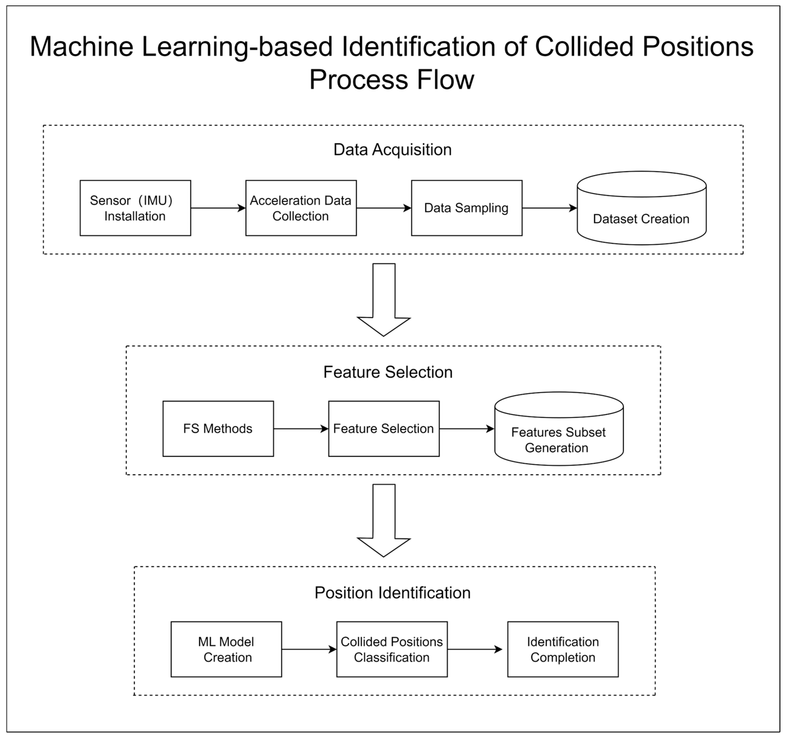
Figure 2.
(A) IMU sensor that collects (X, Y, Z) axis acceleration data. (B) Where and how to install an IMU sensor on the door of the container.
Figure 2.
(A) IMU sensor that collects (X, Y, Z) axis acceleration data. (B) Where and how to install an IMU sensor on the door of the container.
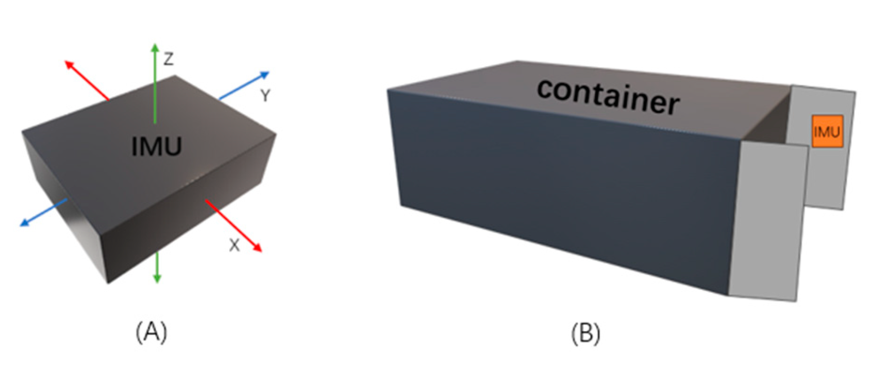
Figure 3.
Raw acceleration data collected by IMU.

Figure 4.
Number of features selected by different FS methods.
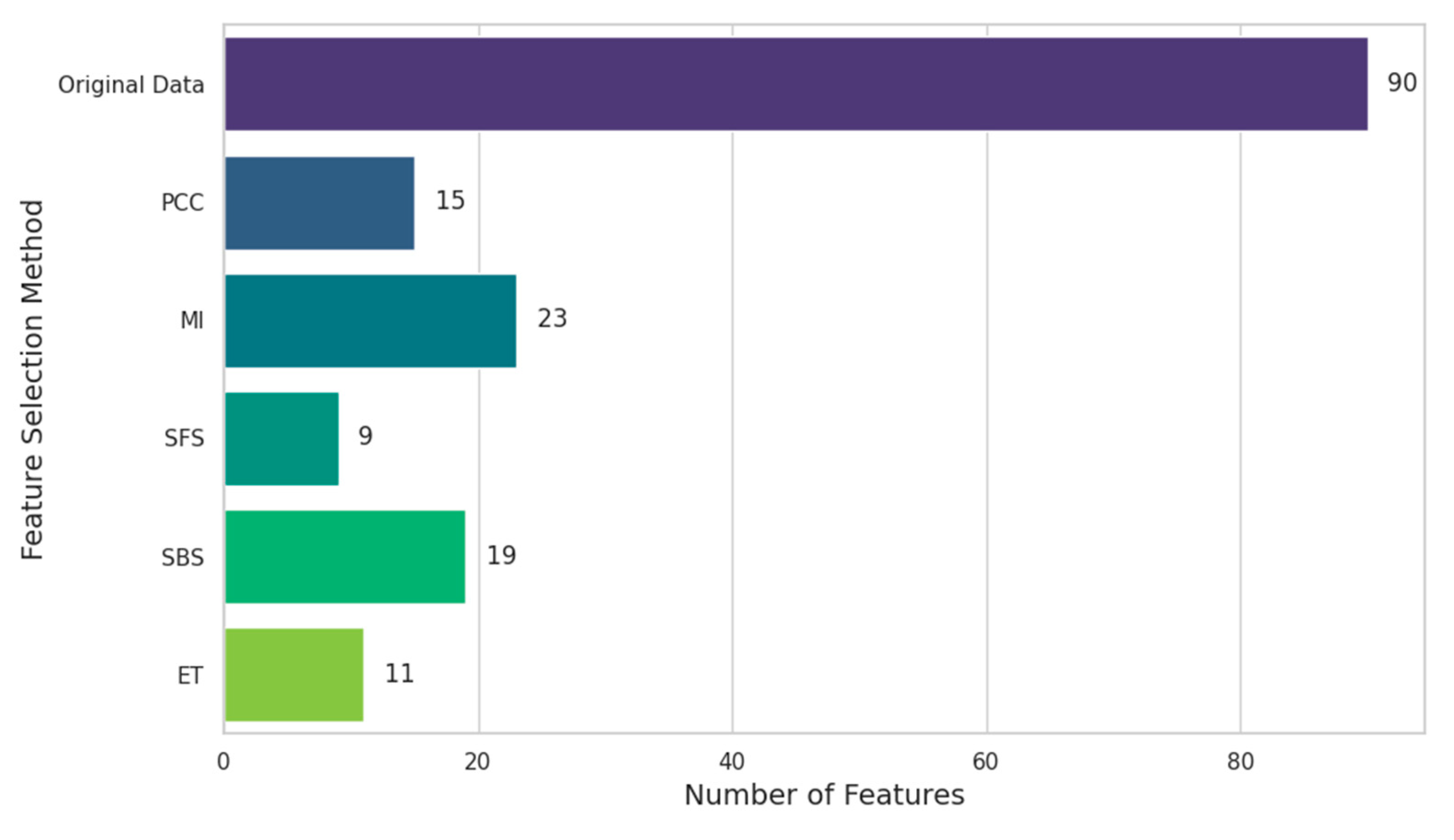
Figure 5.
Histogram of the number of features selected by different FS methods for different categories.
Figure 5.
Histogram of the number of features selected by different FS methods for different categories.
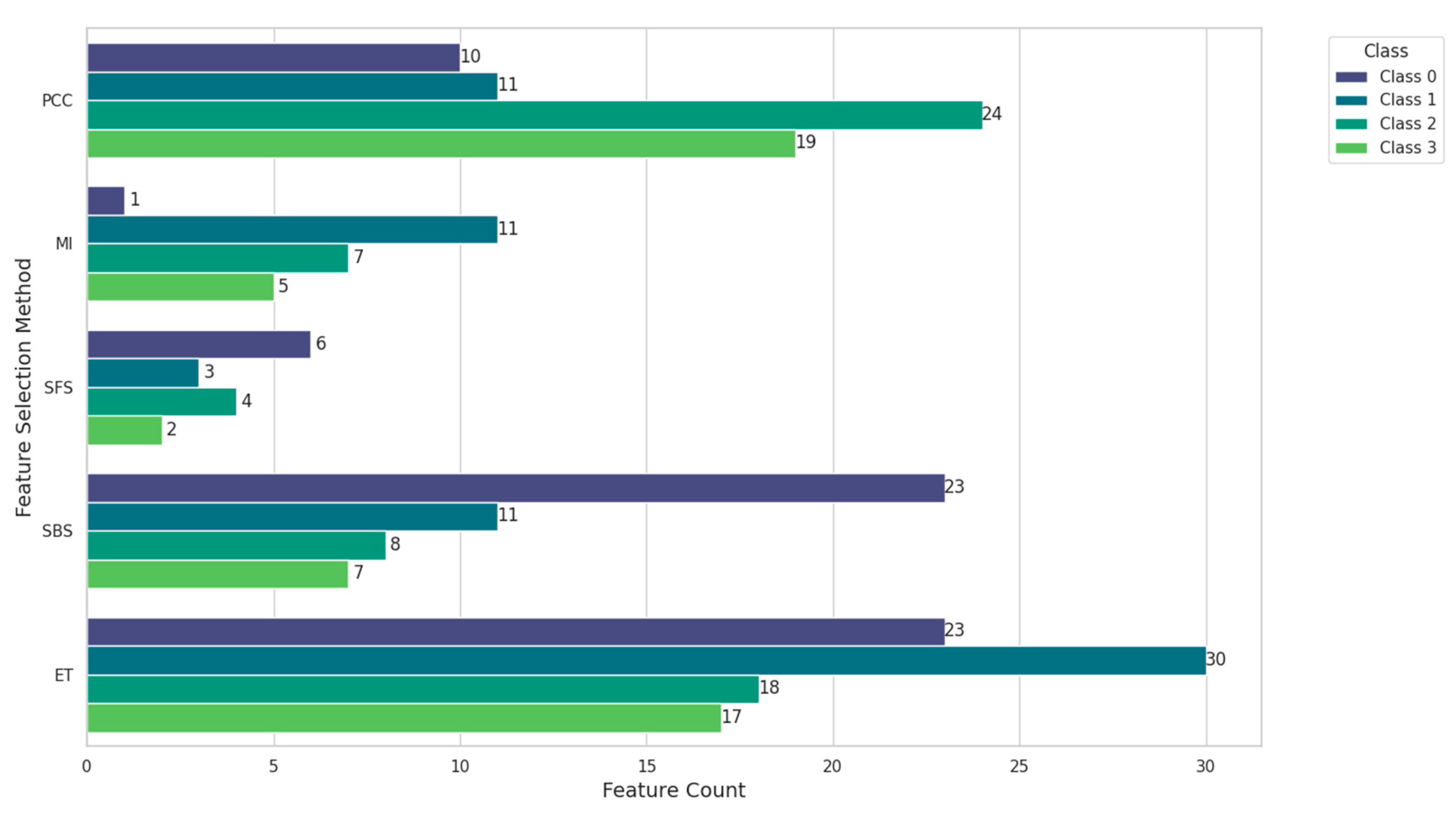
Figure 6.
Classification accuracy heat maps of the 4 class systems.
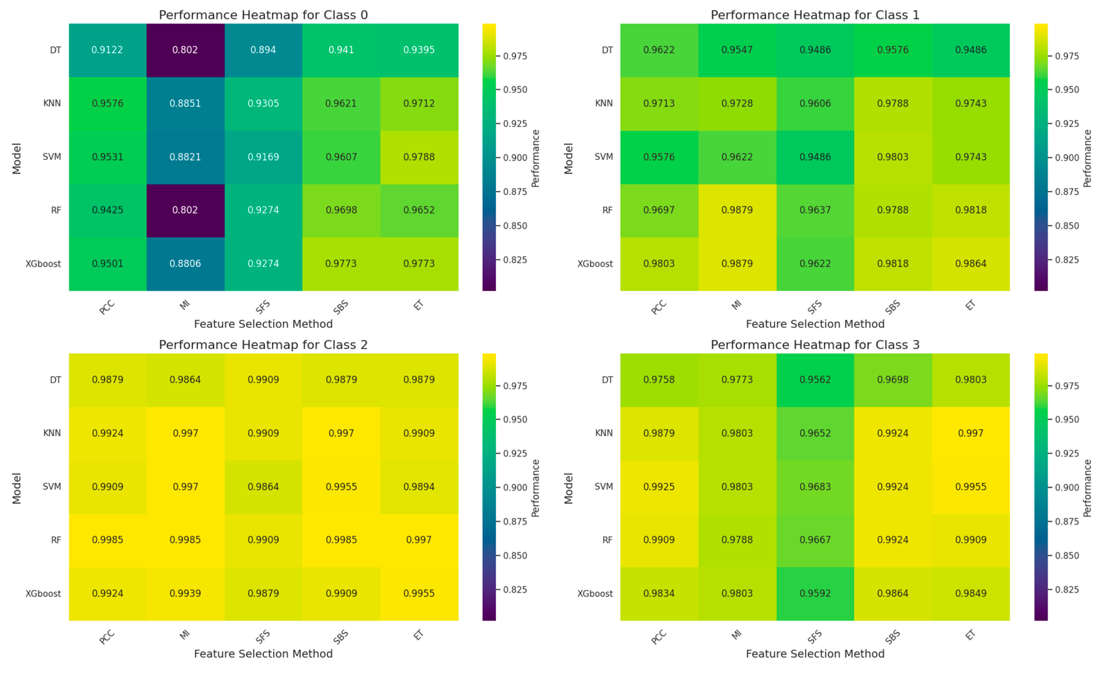
Figure 7.
Data distribution after PCA dimensionality reduction for each category of data.
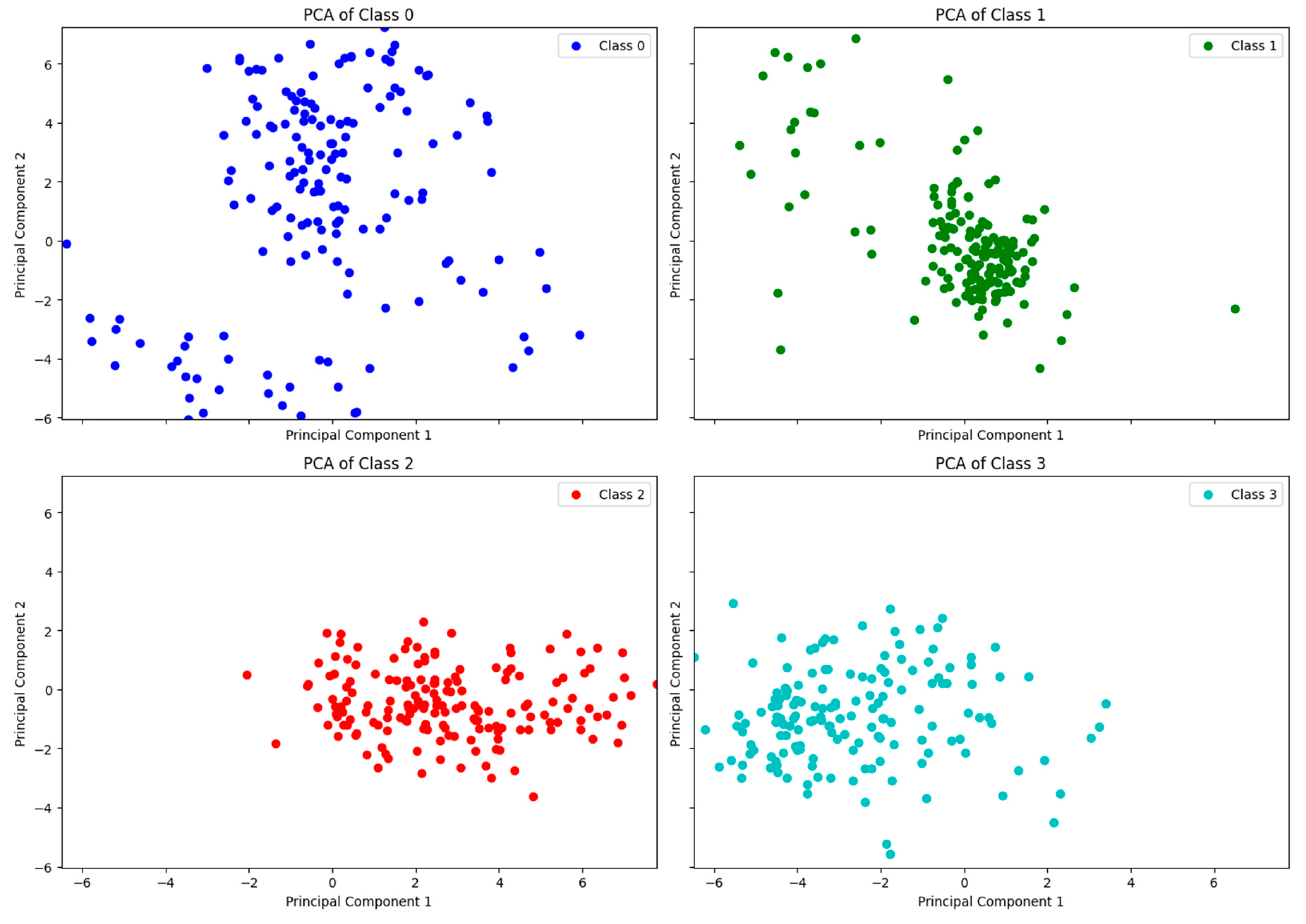

Table 1.
Data format obtained after sampling.
| x1 | y1 | z1 | x2 | … | z30 | Class |
| -1.798331 | -0.858964 | -7.299535 | -3.915565 | … | -0.146063 | 0 |
| -0.003379 | -0.051092 | -0.002288 | -0.237433 | … | 0.063633 | 1 |
| … |
Table 2.
Accuracy of different FS methods and ML models.
| Model | Original | PCC | MI | SFS | SBS | ET |
| DT | 0.9304 | 0.9351 | 0.9410 | 0.9440 | 0.9274 | 0.9334 |
| KNN | 0.9288 | 0.9289 | 0.9667 | 0.9455 | 0.9667 | 0.9712 |
| SVM | 0.9485 | 0.9516 | 0.9697 | 0.9501 | 0.9713 | 0.9697 |
| RF | 0.9803 | 0.9652 | 0.9804 | 0.9607 | 0.9773 | 0.9803 |
| XGBoost | 0.9849 | 0.9652 | 0.9834 | 0.9592 | 0.9849 | 0.9834 |
Table 3.
Execution time for classifying raw data and each FS data with ML models.
| Model | Original | PCC | MI | SFS | SBS | ET |
| DT | 0.2410s | 0.0480s | 0.0690s | 0.0310s | 0.0580s | 0.0350s |
| KNN | 0.1327s | 0.0350s | 0.0340s | 0.0290s | 0.0338s | 0.0300s |
| SVM | 0.6990s | 0.2810s | 0.2760s | 0.1950s | 0.2350s | 0.1640s |
| RF | 2.3920s | 1.1780s | 1.3140s | 1.1370s | 1.3020s | 1.0990s |
| XGBoost | 1.9660s | 0.7510s | 0.7970s | 0.6740s | 0.7510s | 0.6240s |
Table 4.
CPU utilization for classifying raw data and each FS data with ML models.
| Model | Original | PCC | MI | SFS | SBS | ET |
| DT | 4.45% | 0.25% | 0.50% | 0.50% | 0.20% | 0.25% |
| KNN | 1.20% | 0.50% | 1.05% | 0.35% | 1.05% | 0.10% |
| SVM | 1.25% | 0.50% | 0.80% | 0.45% | 0.60% | 3.40% |
| RF | 2.45% | 1.65% | 1.80% | 1.70% | 1.90% | 1.65% |
| XGBoost | 25.40% | 15.55% | 16.55% | 14.75% | 15.80% | 14.35% |
Table 5.
Accuracy of different FS methods and ML models on Class 0 data.
| Model | PCC | MI | SFS | SBS | ET |
| DT | 0.9122 | 0.8020 | 0.8940 | 0.9410 | 0.9395 |
| KNN | 0.9576 | 0.8851 | 0.9305 | 0.9621 | 0.9712 |
| SVM | 0.9531 | 0.8821 | 0.9169 | 0.9607 | 0.9788 |
| RF | 0.9425 | 0.8020 | 0.9274 | 0.9698 | 0.9652 |
| XGBoost | 0.9501 | 0.8806 | 0.9274 | 0.9773 | 0.9773 |
Table 6.
Execution time of different FS methods and ML models on Class 0 data.
| Model | PCC | MI | SFS | SBS | ET |
| DT | 0.0350s | 0.0130s | 0.0300s | 0.0600s | 0.0340s |
| KNN | 0.0310s | 0.0230s | 0.0270s | 0.0340s | 0.0320s |
| SVM | 0.1460s | 0.1670s | 0.1400s | 0.1740s | 0.1270s |
| RF | 1.1260s | 0.7630s | 0.9810s | 1.2820s | 1.0470s |
| XGBoost | 0.2400s | 0.2170s | 0.2300s | 0.2910s | 0.2190s |
Table 7.
CPU utilization of different FS methods and ML models on Class 0 data.
| Model | PCC | MI | SFS | SBS | ET |
| DT | 0.45% | 0.20% | 0.30% | 0.45% | 0.25% |
| KNN | 0.20% | 0.45% | 0.15% | 0.85% | 0.20% |
| SVM | 0.40% | 0.90% | 0.50% | 0.45% | 0.40% |
| RF | 1.70% | 1.40% | 1.70% | 1.85% | 1.75% |
| XGBoost | 7.75% | 6.95% | 7.80% | 8.50% | 7.45% |
Table 8.
Accuracy of different FS methods and ML models on Class 1 data.
| Model | PCC | MI | SFS | SBS | ET |
| DT | 0.9622 | 0.9547 | 0.9486 | 0.9576 | 0.9486 |
| KNN | 0.9713 | 0.9728 | 0.9606 | 0.9788 | 0.9743 |
| SVM | 0.9576 | 0.9622 | 0.9486 | 0.9803 | 0.9743 |
| RF | 0.9697 | 0.9879 | 0.9637 | 0.9788 | 0.9818 |
| XGBoost | 0.9803 | 0.9879 | 0.9622 | 0.9818 | 0.9864 |
Table 9.
Execution time of different FS methods and ML models on Class 1 data.
| Model | PCC | MI | SFS | SBS | ET |
| DT | 0.0310s | 0.0550s | 0.0160s | 0.0350s | 0.0480s |
| KNN | 0.0310s | 0.0310s | 0.0250s | 0.0300s | 0.0320s |
| SVM | 0.1640s | 0.1290s | 0.0860s | 0.1020s | 0.1440s |
| RF | 1.0710s | 1.1080s | 0.7050s | 1.0040s | 1.1020s |
| XGBoost | 0.2020s | 0.1880s | 0.1820s | 0.1890s | 0.1960s |
Table 10.
CPU utilization of different FS methods and ML models on Class 1 data.
| Model | PCC | MI | SFS | SBS | ET |
| DT | 0.35% | 0.30% | 0.30% | 0.30% | 0.20% |
| KNN | 0.25% | 0.30% | 0.30% | 0.15% | 0.40% |
| SVM | 0.40% | 0.40% | 0.25% | 0.50% | 0.50% |
| RF | 1.70% | 1.90% | 1.30% | 1.60% | 1.65% |
| XGBoost | 6.65% | 6.70% | 6.80% | 6.85% | 7.15% |
Table 11.
Accuracy of different FS methods and ML models on Class 2 data.
| Model | PCC | MI | SFS | SBS | ET |
| DT | 0.9879 | 0.9864 | 0.9909 | 0.9879 | 0.9879 |
| KNN | 0.9924 | 0.9970 | 0.9909 | 0.9970 | 0.9909 |
| SVM | 0.9909 | 0.9970 | 0.9864 | 0.9955 | 0.9894 |
| RF | 0.9985 | 0.9985 | 0.9909 | 0.9985 | 0.9970 |
| XGBoost | 0.9924 | 0.9939 | 0.9879 | 0.9909 | 0.9955 |
Table 12.
Execution time of different FS methods and ML models on Class 2 data.
| Model | PCC | MI | SFS | SBS | ET |
| DT | 0.0310s | 0.0160s | 0.0130s | 0.0170s | 0.0170s |
| KNN | 0.0346s | 0.0270s | 0.0250s | 0.0280s | 0.0290s |
| SVM | 0.1460s | 0.0600s | 0.0540s | 0.0670s | 0.0700s |
| RF | 1.0690s | 0.7620s | 0.7130s | 0.7580s | 0.8440s |
| XGBoost | 0.1610s | 0.1300s | 0.1570s | 0.1300s | 0.1320s |
Table 13.
CPU utilization of different FS methods and ML models on Class 2 data.
| Model | PCC | MI | SFS | SBS | ET |
| DT | 0.20% | 0.25% | 0.05% | 0.25% | 0.30% |
| KNN | 1.00% | 0.15% | 0.35% | 0.05% | 0.10% |
| SVM | 0.65% | 0.35% | 0.25% | 0.30% | 0.25% |
| RF | 1.65% | 1.35% | 1.20% | 1.50% | 1.25% |
| XGBoost | 6.25% | 5.45% | 6.25% | 5.60% | 5.50% |
Table 14.
Accuracy of different FS methods and ML models on Class 3 data.
| Model | PCC | MI | SFS | SBS | ET |
| DT | 0.9758 | 0.9773 | 0.9562 | 0.9698 | 0.9803 |
| KNN | 0.9879 | 0.9803 | 0.9652 | 0.9924 | 0.9970 |
| SVM | 0.9925 | 0.9803 | 0.9683 | 0.9924 | 0.9955 |
| RF | 0.9909 | 0.9788 | 0.9667 | 0.9924 | 0.9909 |
| XGBoost | 0.9834 | 0.9803 | 0.9592 | 0.9864 | 0.9849 |
Table 15.
Execution time of different FS methods and ML models on Class 3 data.
| Model | PCC | MI | SFS | SBS | ET |
| DT | 0.0240s | 0.0130s | 0.0110s | 0.0150s | 0.0180s |
| KNN | 0.0340s | 0.0260s | 0.0230s | 0.0280s | 0.0310s |
| SVM | 0.1320s | 0.0640s | 0.0550s | 0.0660s | 0.0860s |
| RF | 1.0080s | 0.7450s | 0.6560s | 0.7910s | 0.8870s |
| XGBoost | 0.1810s | 0.1550s | 0.1720s | 0.1580s | 0.1610s |
Table 16.
CPU utilization of different FS methods and ML models on Class 3 data.
| Model | PCC | MI | SFS | SBS | ET |
| DT | 0.10% | 0.45% | 0.35% | 0.30% | 0.10% |
| KNN | 0.95% | 0.20% | 0.20% | 0.35% | 0.55% |
| SVM | 5.25% | 0.15% | 0.30% | 0.20% | 0.40% |
| RF | 1.80% | 1.30% | 1.05% | 1.50% | 1.45% |
| XGBoost | 6.85% | 5.80% | 6.40% | 6.25% | 6.25% |
Table 17.
Best combinations and their performances.
| System | Model(FS) | Accuracy | Time | CPU |
| Class 0 | KNN(PCC) | 0.9576 | 0.0310s | 0.20% |
| Class 1 | KNN(SBS) | 0.9788 | 0.0300s | 0.15% |
| Class 2 | DT(SFS) | 0.9909 | 0.0130s | 0.05% |
| Class 3 | DT (ET) | 0.9803 | 0.0180s | 0.10% |
Disclaimer/Publisher’s Note: The statements, opinions and data contained in all publications are solely those of the individual author(s) and contributor(s) and not of MDPI and/or the editor(s). MDPI and/or the editor(s) disclaim responsibility for any injury to people or property resulting from any ideas, methods, instructions or products referred to in the content. |
© 2025 by the authors. Licensee MDPI, Basel, Switzerland. This article is an open access article distributed under the terms and conditions of the Creative Commons Attribution (CC BY) license (http://creativecommons.org/licenses/by/4.0/).
Copyright: This open access article is published under a Creative Commons CC BY 4.0 license, which permit the free download, distribution, and reuse, provided that the author and preprint are cited in any reuse.


