
Submitted:
15 August 2023
Posted:
16 August 2023
You are already at the latest version
Abstract
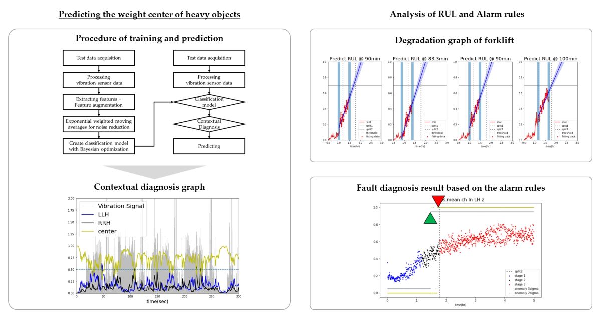
This study examined ways to prevent failures in the front-end of forklifts by addressing the center of gravity of heavy objects carried by forklifts, predicting the remaining useful lifetime (RUL), and the fault diagnosis based on alarm rules. In the research process, acceleration signals were acquired from the outer beam of the front-end of the forklift. A one-second window was applied to extract the time-domain statistical features, which were then set as variables. An exponentially weighted moving average was used to smooth the noise in the feature data set. The AWGN and LSTM autoencoders were used for data augmentation. Based on them, random forest and lightGBM models were used to develop classification models for the weight center of heavy objects carried by a forklift. In addition, contextual diagnosis performed by applying exponentially weighted moving averages to the classification probabilities of the machine learning models showed that random forest achieved an accuracy of 0.9563 and lightGBM achieved an accuracy of 0.9566. In addition, the acceleration data were collected through experiments to predict forklift failure and RUL because of the repeated forklift use when the center of heavy objects carried by the forklift was skewed to the right. The time-domain statistical features of the acceleration signals were extracted and set as variables by applying a 20-second window. Subsequently, logistic regression and random forest models were used to classify the failure stages of the forklifts. The f1-score (macro) obtained were 0.9790 and 0.9220 for logistic regression and random forest, respectively. In addition, the random forest probabilities for each stage were combined and averaged to generate a degradation curve and derive the failure threshold. The coefficient of the exponential function was calculated using the least squares method on the degradation curve, and the RUL prediction model was developed to predict the failure point. In addition, the SHAP algorithm was used to identify the significant features in classifying the stage. The alarm rule-based fault diagnosis was performed using the threshold of the normal stage distribution of the significant features.
Keywords:
PHM
; CBM
; diagnosis
; lightGBM
; random forest
; contextual diagnosis
; RUL
; forklift
1. Introduction
This paper addresses the problem of preventing durability degradation and predicting the failure of forklifts operating in harsh environments. The American Society of Mechanical Engineers (ASME) classifies a forklift as a vehicle that can be driven by a powertrain to carry, push, pull, lift, or stack objects. Forklifts often experience degradation in durability and performance as they move heavy loads in logistics warehouses, factories, construction sites, and other environments. This increases the service and maintenance costs, posing safety risks and potentially harming human life. Prognostics and health management (PHM) technologies are required to prevent these problems and increase utilization [1,2,3]. Traditional reliability analysis uses the mean time to failure data and failure probability distributions to predict the lifetime of a facility. This paper proposes PHM techniques using machine learning and deep learning to classify and predict failures by observing the changes in forklift status using measured data from forklifts. The study aims to improve the durability of forklifts, reduce maintenance costs, and prevent safety accidents using the proposed method.
The Industrial Vehicle Association (ITA) classifies forklifts into eight product families from Class I to Class VIII according to usage characteristics and structural differences. This investigation conducted a PHM study on the front-end structure that lifts heavy loads, which is the core device of ITA CLASS I type electric counterbalance forklifts. The most significant safety hazard with forklifts is vehicle rollovers. These rollovers are common when handling heavy objects that exceed the forklift capacity or when heavy objects are unbalanced and not centered. In addition, when forklifts are used under the condition of repeated unbalanced heavy objects carried by the forklifts, it degrades their performance, which accumulates and leads to safety accidents. This problem was solved using machine learning and deep learning techniques to diagnose the loading status of heavy objects and predict the remaining useful lifetime (RUL) of equipment under repeated loading.
First, vibration data was collected at weight imbalance conditions to conduct the center of heavy objects classification study. The purpose of the classification study was to diagnose the weight imbalance, which is a factor affecting the durability of forklifts. This study aimed to prevent the durability degradation factors in forklifts and reduce the risk of vehicle rollover. In addition, vibration and sound data were collected from forklifts operating under abnormal weight imbalance conditions, and data label classification was performed. Based on this, this study developed a RUL prediction model. Furthermore, fault diagnosis was conducted based on alarm rules to enable the early detection of front-end failures. Through this approach, this study proposed an efficient PHM method to diagnose and prevent durability degradation factors in forklifts, vehicle rollover, and structural failure. The aim of this method was to provide improved operational services for forklifts.
2. Diagnosing and classifying the weight center of heavy objects carried by forklifts
2.1. Experimental data acquisition and feature engineering
This chapter discusses the diagnosis of weight imbalances, one factor that deteriorates the durability of forklifts. Vibration (acceleration) data were acquired from the forklift’s front-end structure and presented a process to diagnose and classify the weight center of heavy objects carried by forklifts. The front-end structure of the forklift consists of a mast, backrest, carriage, and forks, as shown in Figure 1, and the acceleration signals were measured from the outer beam of the mast.
In the measurement experiment for data acquisition, the weight center of heavy objects carried by the forklift was measured in three configurations: Center, Left, and Right. The condition segments of the dataset were classified and organized into Center, Left, and Right according to each center of gravity condition. Two embedded devices (one on the left and one on the right) were attached to the front-end structure of the forklift truck to measure the vibration acceleration in three axes (x, y, z) (sampling rate 500hz), as shown in Figure 2. Considering the load conditions under which the forklift operates, the operating environments of the two datasets (Datasets 1 and 2) were simulated in the experiments while maintaining a state that includes ground noise. In Dataset 1 (only driving mode), the vehicle was loaded with 3,200kg of weight and traveled 80m at maximum speed, as shown on the left in Figure 3. All measurements were taken for approximately 20 minutes per Center, Left, and Right condition segment to eliminate data imbalances within condition segments. In Data Set 2 (complex mode), the forklift made a round trip of 80 meters, as shown on the right in Figure 3, and added lifting, lowering, and back-and-forth tilting tasks at the end of the trip. In Dataset 2, approximately 32 minutes of data were acquired, which is 12 minutes longer than in Dataset 1. Similarly, approximately 32 minutes of data were acquired for the Center, Left, and Right condition segments to eliminate the data imbalance.
Six acceleration signals (2 sensors × (x, y, z accelerations)) were included in Data sets 1 and 2. In Dataset 2, for one acceleration signal, 960,000 feature vectors were collected at 500(Hz) x 32(min) x 60(sec/min). Given the large data size, which could lead to inefficient analysis, this study referred to previous studies [4,5] to handle the data. Eight features were extracted from each window at one-second intervals: min, max, peak to peak, mean (abs), rms (root mean square), variance, kurtosis, and skewness. In addition, four features were added by combining the max, rms, and mean (abs) features: crest factor, shape factor, impulse factor, and margin factor, as listed in Table 1.
Through the above process, 12 features were extracted, and the measured data were compressed for efficient analysis. The data compression process transformed the dimensionality of the data from 960,000×6×1 to 1,920×6×12. In this way, the number of feature vectors in the data was reduced, but the number of features was increased twelvefold, resulting in 72 features. The aim was to enable effective data processing and facilitate the diagnosis of the weight center of heavy objects at a one-second interval. Furthermore, the data range of the feature vectors was scaled from 0 to 1 using min–max normalization. Furthermore, an exponentially weighted moving average with a window size of 2 to 3 seconds was used to smooth the noise signals of the generated features. This approach helped minimize the noise and outliers in the feature data.
The moving average is a method that averages the influence of past data, while the exponentially weighted moving average attenuates that influence exponentially. The moving average is used primarily for time series forecasting and noise reduction [6,7]. The exponentially weighted moving average is used, where the alpha value is adjusted based on the window size, as shown in Equation 1. This approach, as described in Equation 3, can minimize the influence of past vectors while smoothing the noise in the feature vectors, minimizing outliers in the feature signals. Table 3 lists the results of the moving average of the ‘min.’ feature among the features of the x-axis acceleration time series acquired from the embedded device installed on the left side of the front-end structure. In addition, signals with rapid changes are smoothed, as shown in Figure 4.
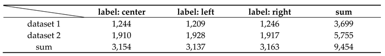
Through the previous feature engineering process, as shown in Table 4, 3,699 feature vectors were generated from Dataset 1 (only driving) for approximately 20 minutes, and 5,755 feature vectors were derived from Dataset 2 (complex mode) measured for approximately 32 minutes. In total, 9,454 datasets were obtained, which were further divided into training and test datasets at a 7:3 ratio. The training and test datasets comprised 6,617 and 2,837 samples, respectively, with each feature vector containing 72 features. An attempt was made to use the training dataset to develop machine learning classifier models and check the performance of the machine learning models on the test dataset.

Table 2.
Table of features before applying the exponentially weighted moving average.
| features | feature vectors without exponentially weighted window | |||||||||
|---|---|---|---|---|---|---|---|---|---|---|
| 1 | … | 101 | 102 | 103 | 104 | 105 | … | m | ||
| Min | . | … | 0.885433 | 0.843096 | 0.797650 | 0.811161 | 0.827289 | … | . | |
| Max | . | … | 0.078264 | 0.080768 | 0.106396 | 0.108621 | 0.116061 | … | . | |
| Peak to Peak | . | … | 0.093902 | 0.112324 | 0.146313 | 0.142308 | 0.140491 | … | . | |
| Mean(abs) | . | … | 0.351697 | 0.401478 | 0.407600 | 0.368202 | 0.429075 | … | . | |
| RMS | . | … | 0.267110 | 0.309412 | 0.318085 | 0.291022 | 0.342365 | … | . | |
| Variance | . | … | 0.073500 | 0.098043 | 0.103476 | 0.086930 | 0.119690 | … | . | |
| Kurtosis | . | … | 0.004885 | 0.008043 | 0.011320 | 0.016485 | 0.014369 | … | . | |
| Skewness | . | … | 0.477752 | 0.469798 | 0.491220 | 0.486768 | 0.492277 | … | . | |
| Crest Factor | . | … | 0.064416 | 0.039363 | 0.096850 | 0.127109 | 0.100406 | … | . | |
| Shape Factor | . | … | 0.049605 | 0.060854 | 0.070667 | 0.080790 | 0.088413 | … | . | |
| Impulse Factor | . | … | 0.033882 | 0.023190 | 0.053079 | 0.070003 | 0.057815 | … | . | |
| Margin Factor | . | … | 0.003583 | 0.002052 | 0.003671 | 0.005534 | 0.003556 | … | . | |
Table 3.
Table of features after applying the exponentially weighted moving average.
| features | feature vectors with exponentially weighted window(3sec) | ||||||||
|---|---|---|---|---|---|---|---|---|---|
| 1 | … | 101 | 102 | 103 | 104 | 105 | … | m | |
| Min | . | … | 0.875394 | 0.859245 | 0.828448 | 0.819804 | 0.823547 | … | . |
| Max | . | … | 0.076663 | 0.078716 | 0.092556 | 0.100588 | 0.108325 | … | . |
| Peak to Peak | . | … | 0.096910 | 0.104617 | 0.125465 | 0.133887 | 0.137189 | … | . |
| Mean(abs) | . | … | 0.365030 | 0.383254 | 0.395427 | 0.381814 | 0.405444 | … | . |
| RMS | . | … | 0.276765 | 0.293089 | 0.305587 | 0.298304 | 0.320335 | … | . |
| Variance | . | … | 0.079095 | 0.088569 | 0.096022 | 0.091476 | 0.105583 | … | . |
| Kurtosis | . | … | 0.005647 | 0.006845 | 0.009082 | 0.012784 | 0.013576 | … | . |
| Skewness | . | … | 0.479047 | 0.474423 | 0.482821 | 0.484795 | 0.488536 | … | . |
| Crest Factor | . | … | 0.052390 | 0.045876 | 0.071363 | 0.099236 | 0.099821 | … | . |
| Shape Factor | . | … | 0.048446 | 0.054650 | 0.062658 | 0.071724 | 0.080069 | … | . |
| Impulse Factor | . | … | 0.027911 | 0.025551 | 0.039315 | 0.054659 | 0.056237 | … | . |
| Margin Factor | . | … | 0.002978 | 0.002515 | 0.003093 | 0.004314 | 0.003935 | … | . |
Table 4.
Configuration of feature vectors in the dataset .
The number of feature vectors in the dataset was also augmented to minimize overfitting during the training process. Data augmentation was performed using Additive White Gaussian Noise (AWGN) and Long Short-Term Memory Autoencoder (LSTM AE), which expanded the training dataset to a maximum of 19,851 samples.
Table 5.
Dataset size based on feature augmentation.
| feature combination | The no. of training data | The no. of test data |
|---|---|---|
| 1. original | 6,617 | 2,837 |
| 2. original + LSTM AE | 13,234 | 2,837 |
| 3. original + AWGN | 13,234 | 2,837 |
| 4. original + LSTM AE +AWGN | 19,851 | 2,837 |
AWGN was applied by referring to prior studies [8], and the target signal-to-noise ratio (SNR) was set to 20 dB. An additional dataset could be generated by mixing noise with the original data, as shown in Figure 5.
An autoencoder is an artificial neural network that can use unlabeled training data to learn a code that efficiently represents the input data. This type of coding is useful for dimensionality reduction because it typically has much lower dimensionality than the input. In particular, it works as a powerful feature extractor that can be used for the unsupervised pre-training of deep neural networks. An autoencoder consists of an encoder that converts the input to an internal representation and a decoder that converts the internal representation back to output [9]. The output result is called reconstruction because the autoencoder reconstructs the input. This study used the mean square error (MSE) as the reconstruction loss in training. LSTM, an artificial recurrent neural network, was designed to address the vanishing gradients in traditional recurrent neural networks (RNNs) [10]. As the number of hidden layers in a neural network and the number of nodes in each layer increase, the last layer is trained while the initial layer is not trained.
This long-term dependency problem arises from the vanishing gradient problem, where the gradients tend to converge to zero during the gradient propagation process, particularly when the data length increases during the training phase of RNNs [11,12]. On the other hand, unlike traditional RNNs, LSTM can effectively overcome the vanishing gradient problem by incorporating long- and short-term state values in the learning process, enabling successful learning even with long training durations [13,14]. In this study, an LSTM autoencoder consisting of two LSTM layers was implemented because time series data were used, as shown in Figure 6. Each layer is used as an encoder and decoder [15]. Furthermore, the repeat vector was used in the decoder part to restore the compressed representation to the original input sequence. The repeat vector function repeats the compressed latent space representation to produce a representation that matches the sequence length. This allows the decoder to use the compressed representation multiple times to reconstruct the original input sequence. Using the LSTM autoencoder, the original feature vectors were trained as input data, and the output vectors were used as the augmentation dataset. The output dataset was generated and replicated to minimize the MSE, resulting in a dataset with similar characteristics and patterns to the input dataset, as shown in Figure 7.
2.2. Classification result
Random forest [16] and lightGBM [17] were chosen as classification algorithms to compare the accuracy of failure prediction. Hyperparameter tuning was performed using ‘Bayesian optimization’. A random forest is an ensemble technique based on decision trees and used as a classifier. Decision trees produce tree-shaped models using input variables and efficiently grow the tree by finding optimal splitting rules at each branch. On the other hand, a single decision tree can suffer from overfitting, which can lead to poor generalization performance. Therefore, the random forest algorithm was used to minimize the overfitting problem.
LightGBM is a machine-learning model based on the Gradient Boosting Decision Tree (GBDT) algorithm. Gradient boosting works by improving the prediction model as new models compensate for the errors of the previous model. Therefore, multiple decision trees can be combined to develop a more robust model that minimizes overfitting. The working mechanism of lightGBM is similar to the conventional GBDT algorithm, but it utilizes the leaf-wise approach during the splitting process (Figure 8). This approach allows lightGBM to produce more unbalanced trees than the traditional level-wise approach, resulting in improved predictive performance. Furthermore, lightGBM includes the feature to perform splitting using only a subset of the data, ensuring faster processing speed for large-scale datasets. However, lightGBM may result in deeper trees, depending on their leaf-wise characteristics and hyperparameter settings, which may lead to deeper trees [18]. While this can improve the prediction accuracy of the training data, it may result in lower accuracy when predicting new data because of the overfitting problem. In the case of lightGBM, the aim was to minimize the overfitting problem through the feature augmentation conducted previously.
Bayesian optimization is a method for finding the optimal solution that maximizes an arbitrary objective function. This optimization technique can be applied to any function for which observations can be obtained and is particularly useful for optimizing black-box functions with high cost and unknown shapes [19]. Therefore, Bayesian optimization is used mainly as a hyperparameter optimization method for machine learning models, taking advantage of the characteristics of such optimization techniques [20]. The optimized hyperparameters were derived through Bayesian optimization, as shown in Figure 9.
Because forklifts move continuously, vibration data has the characteristics of time series data. The time series data and the state changes in the condition segment (center of heavy objects carried by forklift) do not depend on the state at a single point in time but on the past values. Therefore, the probability of classifying the conditioning segment was the exponentially weighted moving average to diagnose the conditioning segment contextually by the moving average instead of diagnosing the conditioning segment only by the probability at that time, as shown in Table 6. Contextual diagnosis in machine learning is a technique to diagnose by considering the context of the given data [21]. This provides a more profound understanding than simply analyzing and predicting data patterns. It simply considers the context of the data before and after, rather than individual data points, to help make an accurate diagnosis. In addition, it is used effectively for outlier detection in time series [22] and partial data [23]. This study attempted to minimize the effect of noise, such as outliers, using the exponentially weighted moving average for contextual diagnosis. In applying contextual diagnosis, this study examined the effects of the window size on the moving average. Figure 10 presents the learning and prediction process flow.
As a result of contextual diagnosis through the exponentially weighted moving average, the classification probability of each condition segment predicted by machine learning changes, as listed in Table 6. Forklifts carry and transport unbalanced heavy objects during continuous movement or operation, and the center of heavy objects does not fluctuate on a one-second basis. Therefore, a two–three-second window was used to calculate the moving average probability. As a result, when the condition segment was diagnosed as “Center”, applying a moving average to the probabilities in certain outlier segments diagnosed as “Left” or “Right” would result in lower values influenced by past data. Figure 11 and Figure 12 present these probabilities as graphs as a function of time. From the observed results, the center of heavy objects carried by the forklift was diagnosed more accurately by the generated classifier.
Because the data imbalance was minimized, the performance was compared using the accuracy score of 24 classifiers, including random forest and lightGBM (Table 7). First, the accuracy increased in all cases as the window size of the exponentially weighted moving average for smoothing the feature vector time series data increased and the alpha value decreased. The classification probabilities of the condition segment predicted by machine learning were subjected to moving average to achieve a contextual diagnosis. In all cases, the classification accuracy of the condition segment increased gradually as the size of the moving average window increased, and the alpha decreased. On the other hand, although the data augmentation minimized the overfitting of the model, it resulted in the same or slightly lower accuracy.
Applying moving average to the probabilities of the lightGBM model resulted in an overall increase in the scores (Case 13-24). This trend can be seen in the probability graphs diagnosing each condition segment in Figure 11 and Figure 12. However, lightGBM, with its leaf-wise growth strategy, tended to overfit with increasing tree depth and often has probabilities highly skewed towards 0 or 1. Therefore, it was difficult to observe performance improvement in the combination of the augmented dataset and contextual diagnosis for the model (Cases 13, 16, 19, and 22).
Compared to lightGBM, random forest exhibited relatively less overfitting and showed gradual fluctuations in probabilities corresponding to changes in the time series. This trend can be observed in Figure 12. The diagnosis of the condition segments was not sigmoidal but rather smooth and gradual because the probability was calculated by averaging the voting values of multiple randomly generated decision trees. These characteristics were expressed in classifiers utilizing the augmented dataset with AWGN and LSTM autoencoders. When applying AWGN and LSTM autoencoder to the dataset and contextual diagnosis in cases 10–12, the application of the probability moving average resulted in a higher score of 0.0331 (3.31%) compared to cases 1–3. On the other hand, the random forest score was lower than lightGBM in all cases when the moving average was not applied (without a contextual diagnosis).
By applying machine learning and contextual diagnosis, the diagnosis of the center of heavy objects carried by forklifts was performed by the condition segment during the process of lifting, tilting, and moving heavy objects on uneven ground using a forklift. As a result, the random forest model (Case 12) achieved a maximum accuracy of 0.9563, while the lightGBM model (Case 24) achieved a maximum accuracy of 0.9566.
3. Abnormal lifting weight stage classification
3.1. Experimental data acquisition and feature engineering
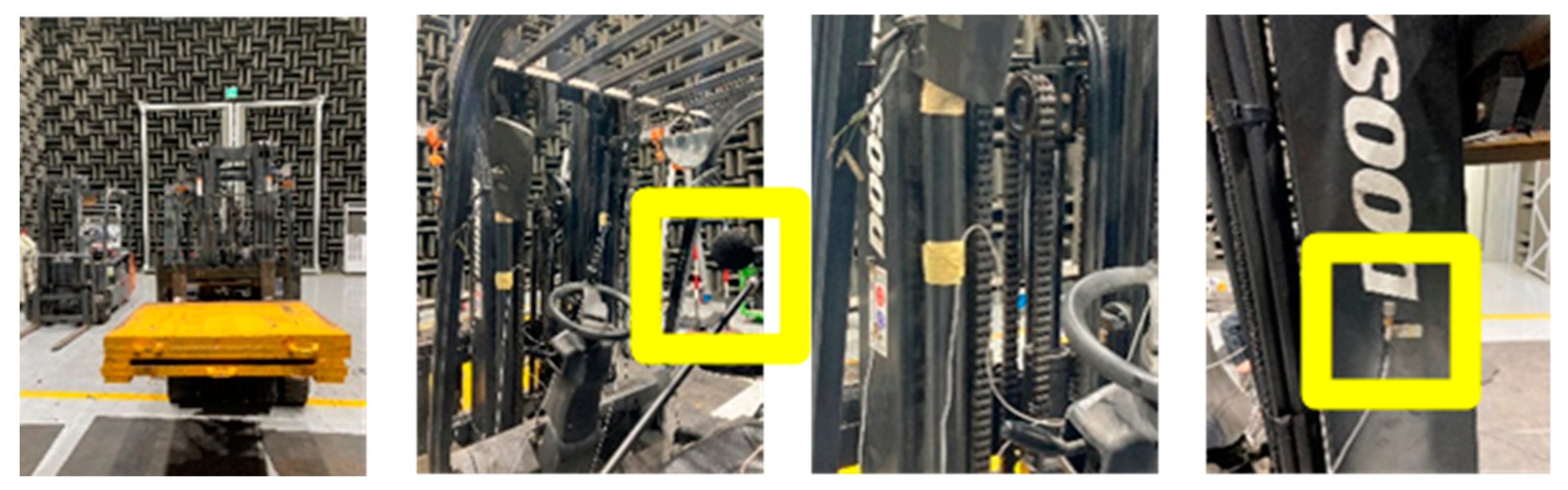
Safety accidents and failure situations were induced by continuous unbalanced heavy objects in a laboratory environment. Data measurements and condition diagnoses were conducted for these situations. During the data measurement process, the forklift repeatedly lifted and lowered an unbalanced load of 1,500kg to the right at a consistent speed every 20 seconds for five hours. The forklift remained stationary throughout this process and did not perform any driving activity. In addition, four 3-axis (x,y,z) acceleration sensors were mounted on the left and right sides of the front-end structure to collect vibration data. Repeated acceleration tests were performed until a failure condition occurred; the forklift swayed, and a loud noise was generated in the structure. In the actual operating environment, it is difficult to diagnose the condition and predict the lifespan by sound because of ambient noise. In this study, a microphone (sampling rate 51.2kHz) was installed at the driver’s position to eliminate ambient noise in an anechoic chamber environment, and labeling was performed using sound data. At the same time, the noise generated was measured by the forklift. These sound data were used to classify and label the failure stages into three stages: normal, failure entry, and failure.
Figure 13.
Images of the repeated abnormal lifting experiment in an anechoic chamber with microphone and vibration sensors.
Figure 13.
Images of the repeated abnormal lifting experiment in an anechoic chamber with microphone and vibration sensors.
The dataset obtained in the experiment contains 12 acceleration signals (four sensors × (x, y, z accelerations)). For each signal of one sensor, 512 (Hz) × 300 (min) × 60 (sec/min) acceleration data were measured, resulting in a total of 9,216,000 data points. In addition, 921,600,000 (51,200 Hz × 300 min × 60 sec/min) sound data were collected. As shown in Figure 14, the plotted sound signal obtained in the time domain made it difficult to track the state changes. By observing the frequency changes over time using the Short-Time Fourier Transform (STFT), it was possible to determine if the forklift was operating over time. On the other hand, state changes and detailed differences were difficult to compare.
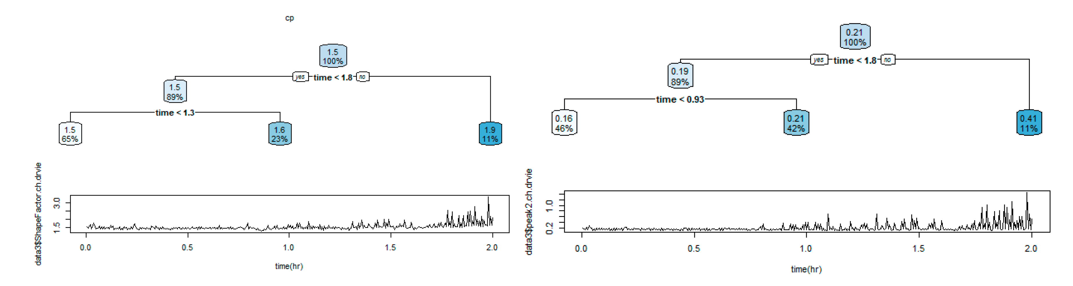
The data size was large, and it was difficult to observe the distinctive state changes when analyzing the raw signals. Twelve features were extracted from the time domain signal, including min, max, peak to peak, mean(abs), rms, variance, kurtosis, skewness, crest factor, shape factor, impulse factor, and margin factor every 20-second window to compress the data and solve these difficulties. Based on this, the dimensions of the acceleration signal and sound signal data were reduced to 900 × 12 × 12 and 900 × 1 × 12, respectively. As reported in chapter 2, an exponentially weighted moving average (alpha 0.5) was applied to the reduced data set to minimize the noise signal in the data. After feature engineering, the CART (Classification and Regression Tree) algorithm [24] was used to classify the failure stages over time using sound features. The CART algorithm is a decision tree algorithm for classification and regression analysis that evaluates the importance of each variable based on the input data and prioritizes the important variables to produce a decision tree. The CART algorithm was used to derive 12 decision trees for each feature by pruning to prevent overfitting and classify the status into three levels. Significant branching points could be derived from eight of the 12 decision trees, and the failure stage was classified based on the average value of the branching points derived from the eight decision trees (Table 8). Based on the classification results, breakpoint 1 was determined to be at 1.18 hours and breakpoint 2 at 1.77 hours, which were used to distinguish the labeling of the data (Table 9). Furthermore, a comparison of the recorded forklift experimental video showed that beyond breakpoint 1, the forklift exhibited early failure symptoms (beginning to shake), demonstrating a complete failure state at breakpoint 2.
Figure 15.
Visualization examples of CART algorithm result.
The 900 data generated were divided into 630 data for training and 270 data for testing. Given that the dataset is imbalanced, the performance was evaluated using the f1-score during the validation process. The f1-score is one of the metrics that evaluate the accuracy of a model and is calculated as the harmonic mean of precision and recall. When data is unbalanced, the prediction accuracy for a small number of data classifications is often high, but the prediction accuracy for a large number of data classifications is often low. In such situations, relying solely on accuracy may give the impression of high prediction accuracy for a small number of data classifications. On the other hand, the accuracy for most data classifications may be relatively lower, leading to inadequate overall model performance evaluation. The f1-score considered both precision and recall, which makes it more suitable for dealing with imbalanced classification problems [25,26,27]. Therefore, when the data is unbalanced, using the f1-score is a more accurate way to evaluate the model performance. Consequently, the f1 score was used to evaluate the performance in this unbalanced data set.
3.2. Stage classification result
Previously, labeling was performed using sound features, and based on this, logistic regression and random forest classifiers were trained using vibration and sound features. The dataset was divided into two cases. Case 1 consisted of 144 features using only vibration features, while Case 2 consisted of 156 features incorporating both vibration and sound features. The sound features were acquired for labeling purposes, but additional cases were produced to assess the improvement in classifier performance when incorporating these features into the training.
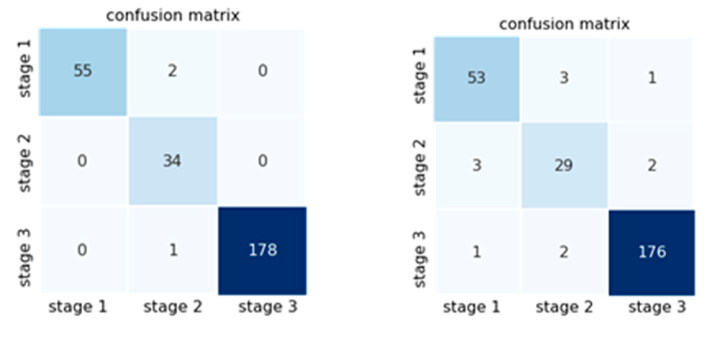
Logistic regression and random forest were chosen as the machine learning models. LightGBM, used in the previous chapter, is prone to overfitting when the data set size is small. LightGBM was deemed inappropriate because this dataset consists of 900 feature vectors and was not used in this study. No additional hyperparameter tuning was conducted, and only the default parameters provided by the scikit-learn module in Python were utilized. Based on the validation results of the test data shown in Table 10, the logistic regression classifier achieved an f1-score (macro) of 0.9599 for Case 1 and 0.9790 for Case 2. In the case of random forest, the f1-score (macro) for Cases 1 and 2 were 0.9116 and 0.9220, respectively. This confirms that it is possible to classify the forklifts as healthy or aging under repeated unbalanced load weight conditions based on acceleration signals.
Figure 16.
Confusion matrix result (left: logistic regression, right: random forest).
4. RUL analysis and alarm rule fault diagnosis in abnormal lifting due to unbalanced load
4.1. Generation of the life prediction model and verification of RUL
The dataset and generated classifiers from Chapter 3 were used to perform RUL prediction and fault diagnosis through alarm rules, known as condition-based management [28]. In the case of logistic regression, as shown in Figure 17, the classification probabilities of the classifier were derived as either 0 or 1, making it difficult to track the progressive changes in the state. Therefore, it was not feasible to adopt degradation graphs for logistic regression. On the other hand, as shown in Chapter 3, when the classification probabilities of the entire dataset belonging to each stage were visualized using a random forest classifier, a gradual change in state was observed in the graph (Figure 18). This represents the degradation state of the forklift using classification probabilities, and the probabilities of Stages 1 and 3 were combined and averaged to generate the degradation graph (Figure 19). After analyzing the degradation graph, Stage 3 was reached after approximately 106 minutes, and the threshold was a probability of 0.7.
The model for RUL was constructed using an exponential function equation, as follows.
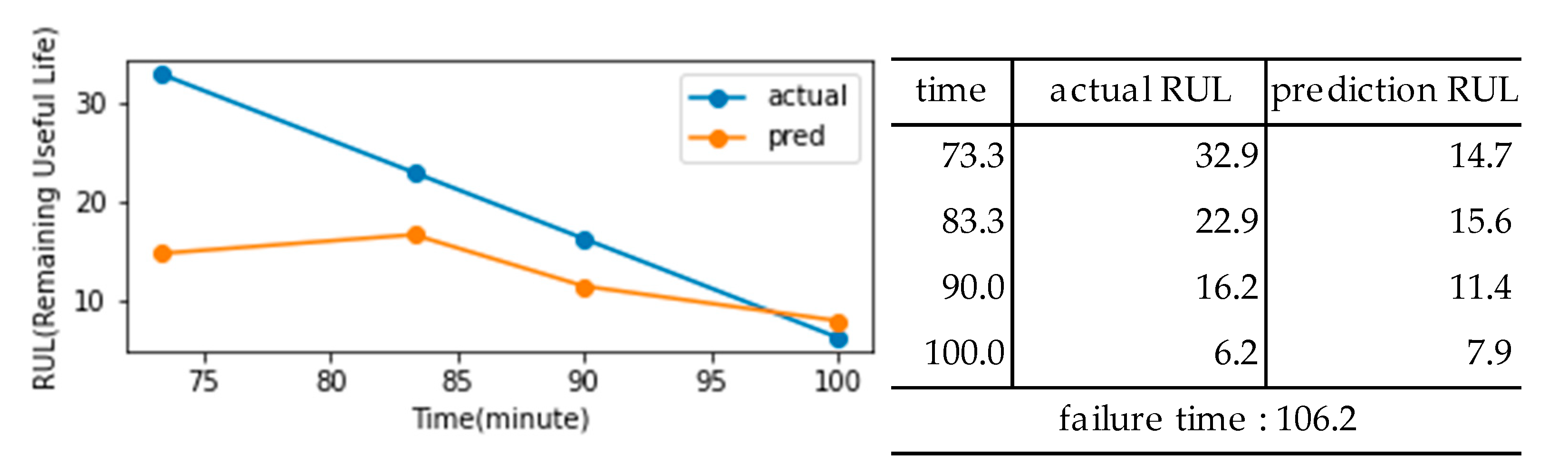
The exponential coefficient was determined using the method of least squares, and the data range to which the method of least squares was applied included the data from the 30 minutes before the diagnostic time. Based on these characteristics, the exponential function continued to change with time, and the time when the y-value of the exponential function reached 0.7 was calculated to analyze the RUL. During the analysis of the RUL, the confidence interval was included by considering to Y(1.1 in the pre- and post-prediction time points. The analysis showed that the early data predicted the failure rather early, as shown in Figure 20. The gap between the actual and the predicted RUL decreased gradually as the failure point approached (Figure 21).
Figure 20.
Degradation graph of forklift using the average probability of a random forest classifier.
Figure 20.
Degradation graph of forklift using the average probability of a random forest classifier.
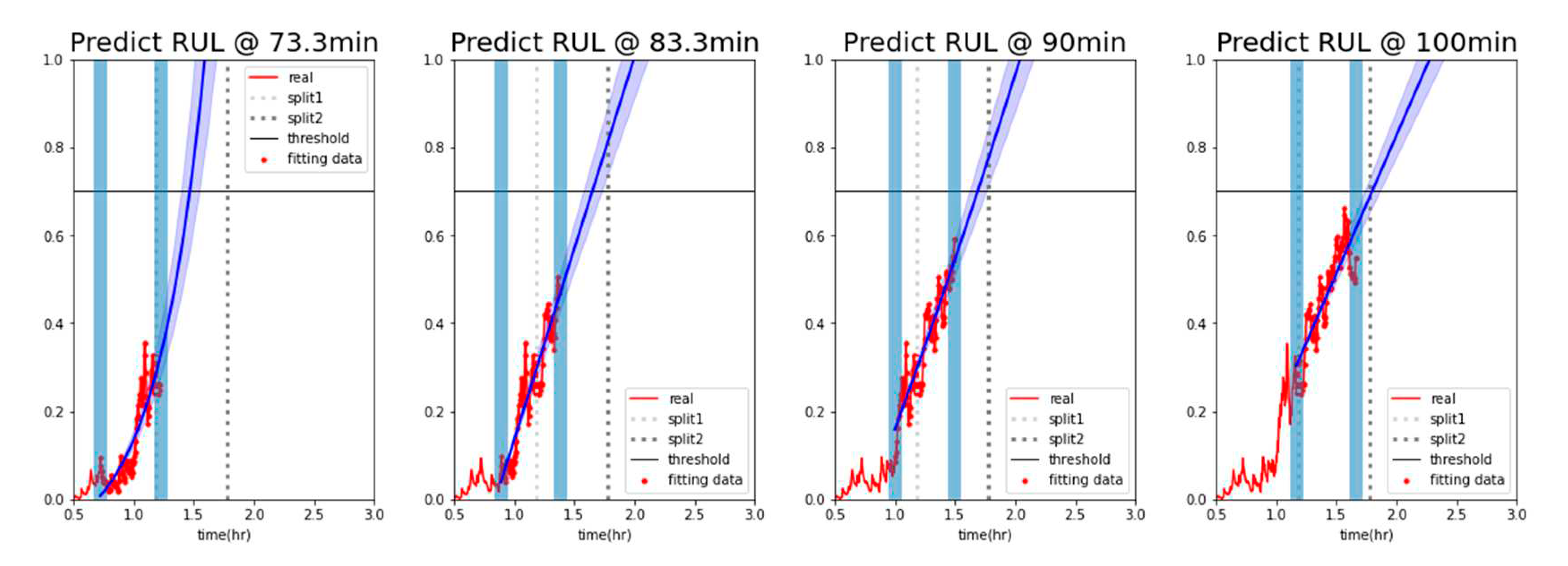
Figure 21.
Remaining Useful Lifetime (RUL) result.
4.2. Alarm rule-based fault diagnosis
The SHAP (SHapley Additive exPlanations) algorithm was used to diagnose faults based on the key features and alarm rules. The goal was to determine which features were critical for state classification using the SHAP algorithm with the previously trained random forest classifier. This analysis allowed the identification of the significant features used for state classification. SHAP is an algorithm used to analyze the contribution of features to the predictions made by machine learning models. It helps determine the importance of each feature in the model’s predictions. The SHAP algorithm considers all features necessary to explain the model predictions and calculates the impact of each feature on the prediction outcome [29]. Calculating the Shapley value for all feature combinations is computationally expensive. Therefore, the SHAP algorithm uses approximations that can be calculated relatively quickly for tree-based models, such as the random forests or XGBoost [29]. The SHAP algorithm provides various interpretation results, such as feature importance, feature contribution, and feature effect, which help interpret the model and explain the prediction results reliably [29]. The SHAP algorithm improves the interpretability of machine learning models and plays a vital role in model developers and helping users understand the model prediction results [29].
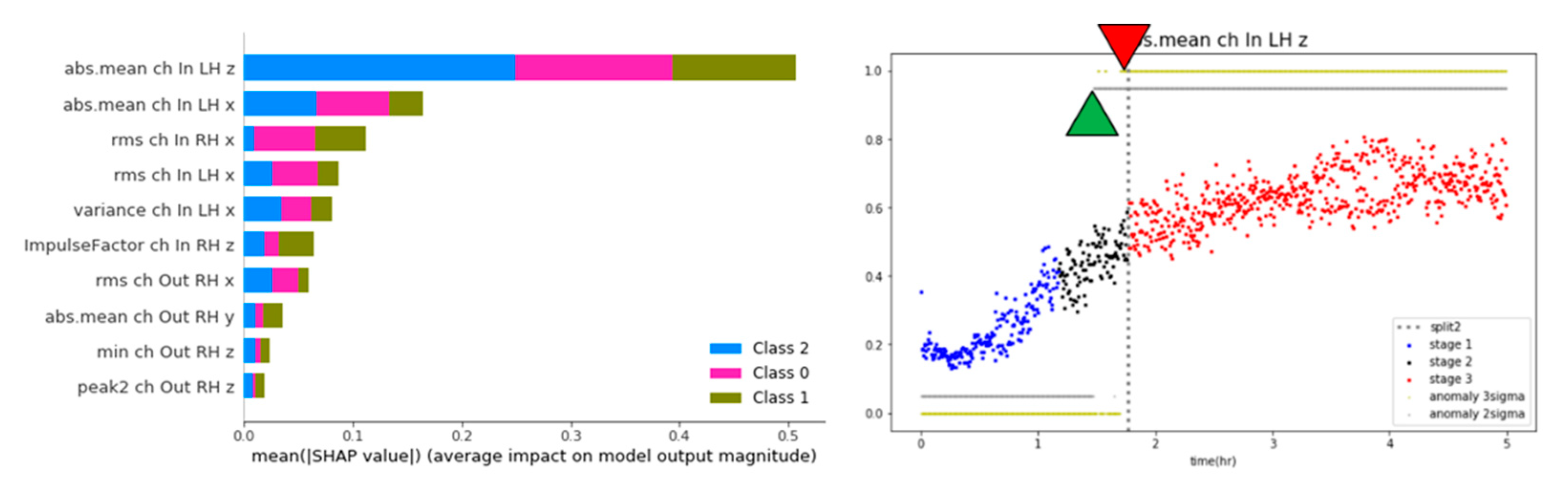
The features that contribute significantly to health diagnostics were identified using the SHAP algorithm. As shown on the left in Figure 20, the ‘abs.mean ch In LH z’ feature contributes the most to the health diagnosis. A progressive state change, similar to the degradation model graph, could be observed by observing the dispersion of the time series of the corresponding feature (Figure 20, right image). The 2-sigma and 3-sigma values of the ‘abs.mean ch In LH z’ feature from the distribution of the normal data range in stage 1. These values were then used as the threshold for fault diagnosis. Next, an alarm rule was set to diagnose a failure when the exponentially weighted moving average value of the feature (alpha 0.17) exceeds a threshold. As shown in Figure 20 (right), the 3-sigma threshold can diagnose failure just before failure, and the 2-sigma threshold can predict failure at the point of the precursor symptoms.
Figure 20.
Results of SHAP and fault diagnosis based on the Alarm rules.
5. Discussion
This study diagnosed the center of heavy objects carried by the forklift to prevent the failure of the forklift front-end. In the research process, this study acquired the acceleration signals during lifting, tilting, and moving heavy objects by the forklift on uneven ground and in various operating environments. Acceleration signals were acquired from the left and right outer beams of the front end of the forklift, and time-domain statistical features were extracted and set as variables by applying a window at one-second intervals. This reduced the number of feature vectors and multiplied the features 12 times for effective data processing and analysis. The data were augmented using AWGN and LSTM autoencoders to minimize overfitting. Based on this, classifiers were developed using the random forest and lightGBM machine learning models to classify the center of heavy objects carried by forklifts while driving and working. Using machine learning and contextual diagnosis based on exponentially weighted moving average, a maximum accuracy of 0.9563 was achieved with the random forest model, and a maximum accuracy of 0.9566 was obtained with the lightGBM model in diagnosing the center of the objects carried by the forklift.
At this time, an exponentially weighted moving average study was conducted to smooth out the noise of the features. As a result, the moving average minimizes outliers without applying complex noise filter techniques, and the accuracy of machine learning increases as the exponentially weighted moving average window size increases. The accuracy increased when the machine learning classification probability for contextual diagnosis was exponentially weighted moving averaged. By applying data augmentation, the overfitting of the model was minimized, and the accuracy score remained comparable or slightly lower. In the lightGBM model, applying the moving average to the classification probabilities showed an overall trend of score improvement. On the other hand, lightGBM is prone to overfitting with increasing tree depth and tends for the classification probability values to be skewed towards 0 or 1. As a result, it was difficult to see a performance improvement in the combination of augmented datasets and contextual diagnostics. On the other hand, in the case of the random forest, there was less overfitting compared to lightGBM, and it exhibited gradually increasing or decreasing classification probabilities according to the time series. These characteristics were observed in the augmented dataset with the application of AWGN and LSTM autoencoder. An average score improvement of 0.0331 (3.31%) was observed by applying the augmented dataset and contextual diagnosis, along with the moving average on the classification probabilities. On the other hand, the random forest score was lower than lightGBM without applying the moving average.
A study was also conducted on predicting the RUL under abnormal conditions and fault diagnosis based on alarm rules to prevent failures in the front end of the forklift. To predict the RUL under repetitive unbalanced load conditions, a 20-second window interval was used to extract the statistical features from the time domain of the acceleration signal and set them as variables. The data were measured in an anechoic chamber. At the same time as the acceleration signal was recorded, the sound signal was recorded by a microphone. These signals were used to analyze the changes in the state of the forklift. The CART algorithm was used to classify and label the statistical features extracted from the sound signals. In addition, the consistency of the labeling was verified by comparing it with the labeling obtained from the recorded videos. Based on the previous labeling results, logistic regression and random forest models were used to classify the failure stages of forklifts. The f1-score (macro) obtained for logistic regression and random forest were 0.9790 and 0.9220, respectively. The logistic regression classifier achieved the highest score among the classifiers. On the other hand, when analyzing the probability change graph of the machine learning classifier, the probability values were skewed toward 0 or 1, making it difficult to track the state changes of the forklift. Therefore, the degradation status of the forklift could be monitored using the classification probabilities generated by the random forest. The results showed a gradual change in the condition of the forklift over time. Based on this, the probabilities generated by the random forest for each stage were combined and averaged to produce a degradation graph. The failure threshold was derived by analyzing the degradation graph. In addition, the degradation graph was used to calculate the coefficients of the exponential function using the least squares method. The failure point was predicted by deriving the RUL prediction model. RUL analysis showed that the accuracy of RUL increases over time. The SHAP algorithm was used to identify the critical features in the stage classification. In addition, the thresholds of the normal stage distribution of the key features were used. As a result, an anomaly diagnosis was performed based on alarm rules.
In summary, a diagnosis of the center of heavy objects carried by the forklift can provide information on operations that may affect the durability of the forklift. This approach will help improve the equipment durability and ensure safety in forklift operation. Equipment operation plans can be established by providing the RUL information of the forklift. In addition, effective equipment maintenance can be achieved by setting the failure level index as the main feature, considering the trade-off optimization of equipment lead time and opportunity cost, and managing forklifts by dividing the threshold level.
Author Contributions
Conceptualization and methodology, J.-G.L. and Y.-S.K.; validation, formal analysis, investigation, and data curation, J.-G.L. and J.-H.L.; research administration, J.-H.L; funding acquisition, J.-H,L. All authors have read and agreed to the published version of the manuscript.
Funding
This research was supported by a grant from the National R&D Project “Development of fixed offshore green hydrogen production technology connected to marine renewable energy” funded by the Ministry of Oceans and Fisheries (1525013967).
Institutional Review Board Statement
Not applicable.
Informed Consent Statement
Not applicable
Data Availability Statement
The data presented in this study are available upon request from the corresponding author. The data derived from the present study are only partially available for research purposes.
Acknowledgments
This research was supported by a grant from the National R&D Project “Development of fixed offshore green hydrogen production technology connected to marine renewable energy” funded by the Ministry of Oceans and Fisheries (1525013967).
Conflicts of Interest
The authors have no conflicts of interest to declare.
References
- Tsui, K.L.; Chen, N.; Zhou, Q.; Hai, Y.; Wang, W. Prognostics and Health Management: A Review on Data Driven Approaches. Math. Probl. Eng. 2015, 2015, 1–17. [Google Scholar] [CrossRef]
- Lee, J. , Wu, F., Zhao, W., Ghaffari, M., Liao, L., & Siegel, D. Prognostics and health management design for rotary machinery systems—Reviews, methodology and applications. Mechanical systems and signal processing 2014, 42, 314–334. [Google Scholar]
- Meng, H.; Li, Y.-F. A review on prognostics and health management (PHM) methods of lithium-ion batteries. Renew. Sustain. Energy Rev. 2019, 116, 109405. [Google Scholar] [CrossRef]
- Ben Ali, J.; Saidi, L.; Harrath, S.; Bechhoefer, E.; Benbouzid, M. Online automatic diagnosis of wind turbine bearings progressive degradations under real experimental conditions based on unsupervised machine learning. Appl. Acoust. 2017, 132, 167–181. [Google Scholar] [CrossRef]
- Saidi, L.; Ali, J.B.; Bechhoefer, E.; Benbouzid, M. Wind turbine high-speed shaft bearings health prognosis through a spectral Kurtosis-derived indices and SVR. Appl. Acoust. 2017, 120, 1–8. [Google Scholar] [CrossRef]
- Holt, C.C. Forecasting seasonals and trends by exponentially weighted moving averages. Int. J. Forecast. 2004, 20, 5–10. [Google Scholar] [CrossRef]
- Hunter, J. S. The exponentially weighted moving average. Journal of quality technology, 1986, 18, 203–210. [Google Scholar] [CrossRef]
- Vaseghi, S. V. Advanced digital signal processing and noise reduction. John Wiley & Sons, 2008.
- Aurélien, G. Hands-on machine learning with Scikit-learn, Keras, and TensorFlow. O’Reilly Media, Inc., 2022.
- Graves, A. Supervised Sequence Labelling with Recurrent Neural Networks. 2012. [Google Scholar] [CrossRef]
- Bengio, Y.; Simard, P.; Frasconi, P. Learning long-term dependencies with gradient descent is difficult. IEEE Trans. Neural Networks 1994, 5, 157–166. [Google Scholar] [CrossRef] [PubMed]
- Pascanu, R. , Mikolov, T., & Bengio, Y. On the difficulty of training recurrent neural networks. In International conference on machine learning (pp. 1310-1318). Pmlr. 20 May.
- Hochreiter, S. The Vanishing Gradient Problem During Learning Recurrent Neural Nets and Problem Solutions. Int. J. Uncertain. Fuzziness Knowl.-Based Syst. 1998, 6, 107–116. [Google Scholar] [CrossRef]
- Gers, F.A.; Schmidhuber, J.; Cummins, F. Learning to Forget: Continual Prediction with LSTM. Neural Comput. 2000, 12, 2451–2471. [Google Scholar] [CrossRef]
- Bao, W.; Yue, J.; Rao, Y. A deep learning framework for financial time series using stacked autoencoders and long-short term memory. PLOS ONE 2017, 12, e0180944. [Google Scholar] [CrossRef]
- Breiman, L. Random forests. Machine learning, 2001, 45, 5–32. [Google Scholar] [CrossRef]
- Ke, G. , Meng, Q., Finley, T., Wang, T., Chen, W., Ma, W.,... & Liu, T. Y. Lightgbm: A highly efficient gradient boosting decision tree. Advances in neural information processing systems, 2017, 30.
- Liang, W.; Luo, S.; Zhao, G.; Wu, H. Predicting Hard Rock Pillar Stability Using GBDT, XGBoost, and LightGBM Algorithms. Mathematics 2020, 8, 765. [Google Scholar] [CrossRef]
- Greenhill, S.; Rana, S.; Gupta, S.; Vellanki, P.; Venkatesh, S. Bayesian Optimization for Adaptive Experimental Design: A Review. IEEE Access 2020, 8, 13937–13948. [Google Scholar] [CrossRef]
- Bergstra, J. , Bardenet, R., Bengio, Y., & Kégl, B. Algorithms for hyper-parameter optimization. Advances in neural information processing systems, 2011, 24.
- Singh, K. , & Upadhyaya, S. Outlier detection: applications and techniques. International Journal of Computer Science Issues (IJCSI), 2012, 9, 307. [Google Scholar]
- Weigend, A. S. , Mangeas, M., & Srivastava, A. N. Nonlinear gated experts for time series: Discovering regimes and avoiding overfitting. International journal of neural systems 1995, 6, 373–339. [Google Scholar] [CrossRef]
- Kou, Y. , Lu, C. T., & Chen, April 2006., D. Spatial weighted outlier detection. In Proceedings of the 2006 SIAM international conference on data mining (pp. 614-618). Society for Industrial and Applied Mathematics. [Google Scholar]
- Breiman, L. Classification and regression trees. Routledge, 2017.
- Sokolova, M. , Japkowicz, N., & Szpakowicz, S. (2006). Beyond accuracy, F-score and ROC: a family of discriminant measures for performance evaluation. In AI 2006: Advances in Artificial Intelligence: 19th Australian Joint Conference on Artificial Intelligence, Hobart, Australia, Proceedings 19 (pp. 1015-1021). Springer Berlin Heidelberg, 4-8 December 2006.
- Jeni, L. A. , Cohn, J. F., & De La Torre, F. Facing imbalanced data--recommendations for the use of performance metrics. In 2013 Humaine association conference on affective computing and intelligent interaction (pp. 245-251). IEEE, 2013. 20 September.
- Sun, Y., Wong, A. K., & Kamel, M. S. Classification of imbalanced data: A review. International journal of pattern recognition and artificial intelligence. 2009, 23, 687–719.
- Kumar, S.; Mukherjee, D.; Guchhait, P.K.; Banerjee, R.; Srivastava, A.K.; Vishwakarma, D.N.; Saket, R.K. A Comprehensive Review of Condition Based Prognostic Maintenance (CBPM) for Induction Motor. IEEE Access 2019, 7, 90690–90704. [Google Scholar] [CrossRef]
- Lundberg, S. M. , & Lee, S. I. A unified approach to interpreting model predictions. Advances in neural information processing systems, 2017, 30.
Figure 1.
Electric-powered counterbalance forklift of ITA CLASS I type.
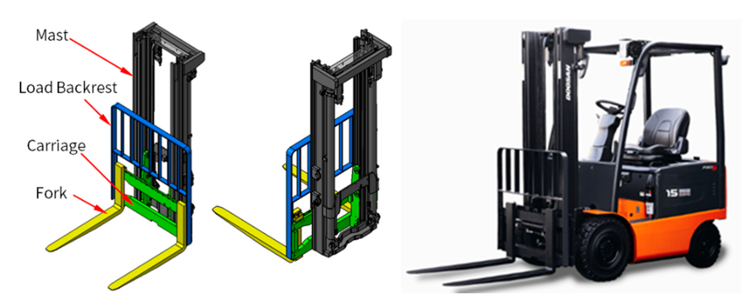
Figure 2.
Data acquisition equipment and 3,200kg weight on a forklift.
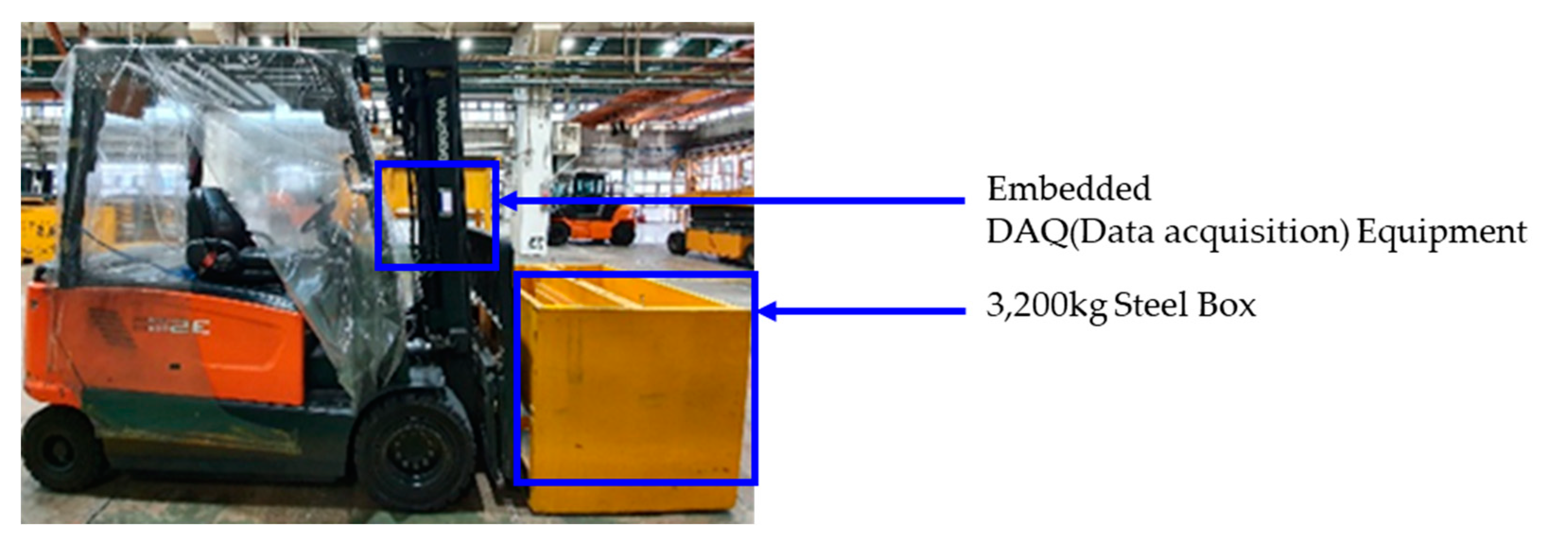
Figure 3.
Description of forklift operation modes for datasets 1(only driving) and 2(complex mode).
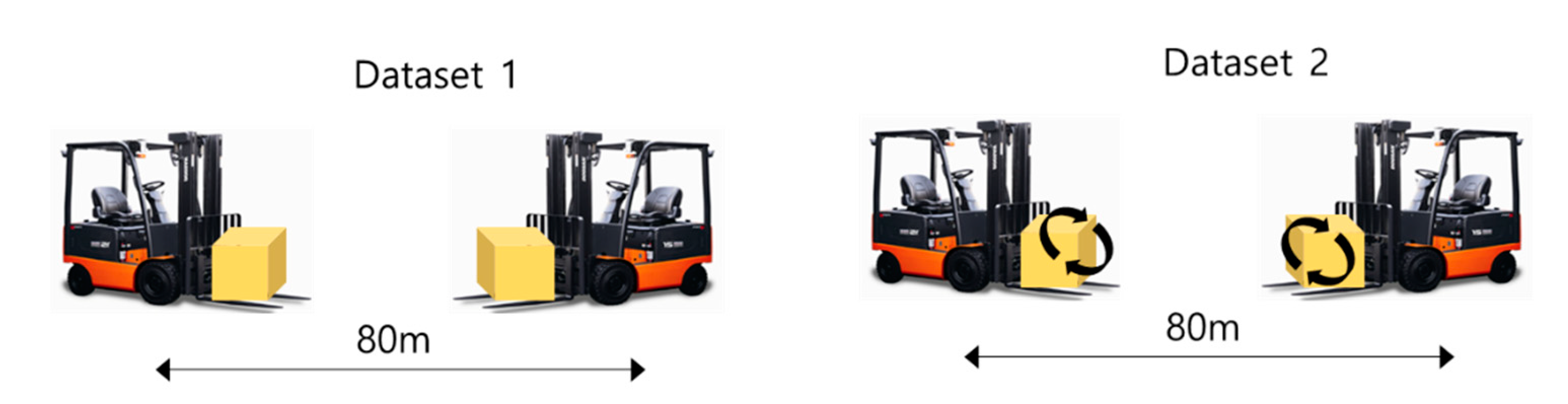
Figure 4.
Exponentially weighted moving average result (‘min.’ feature of the left x-axis acceleration signal).
Figure 4.
Exponentially weighted moving average result (‘min.’ feature of the left x-axis acceleration signal).
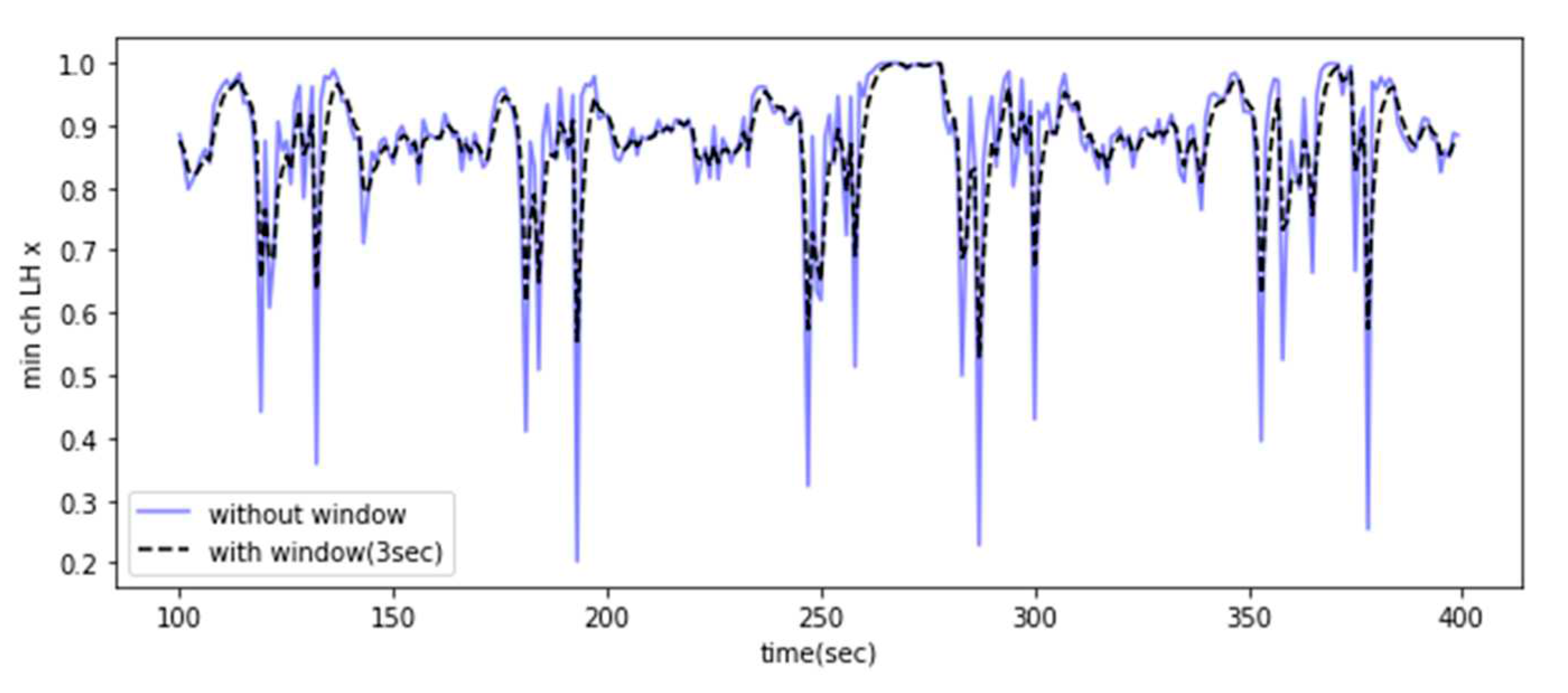
Figure 5.
Results of noise mixed augmentation using AWGN (Additive White Gaussian Noise).
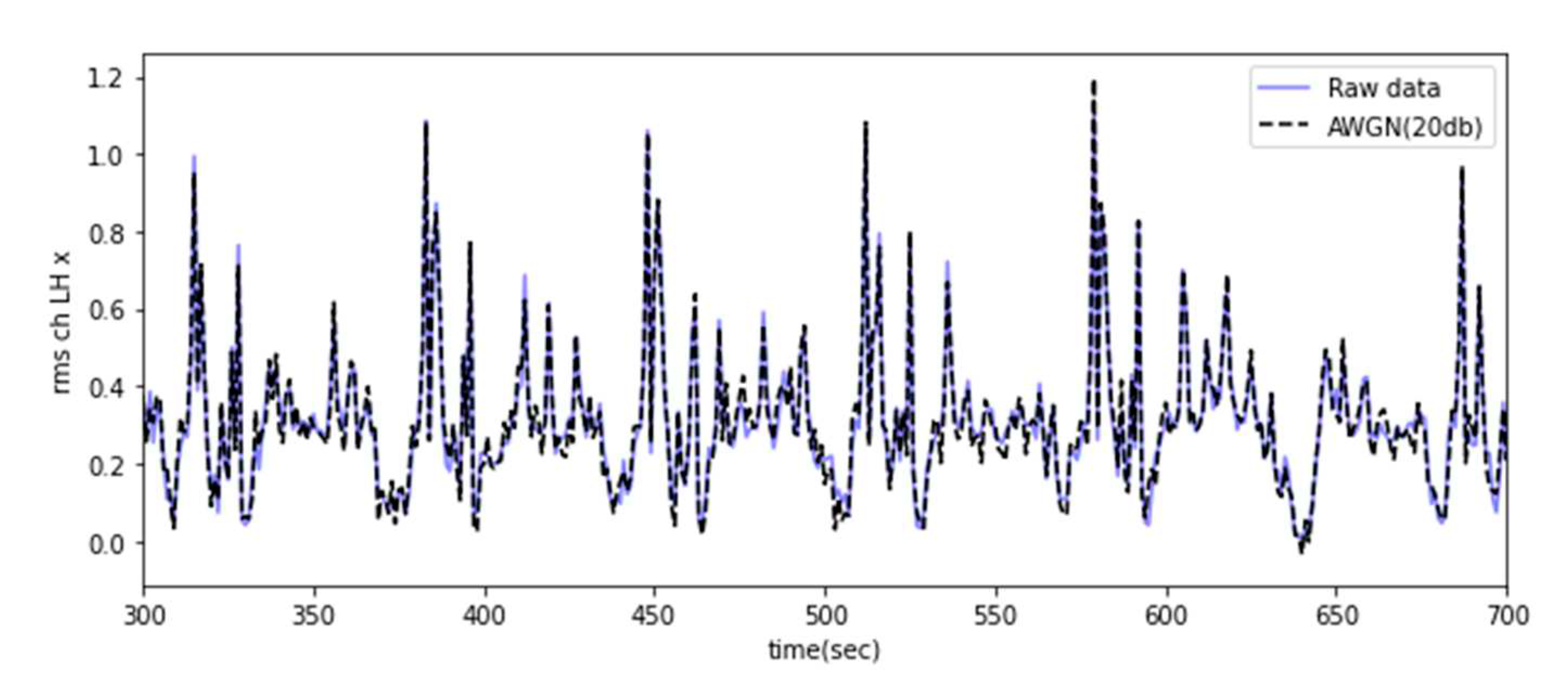
Figure 6.
Structure of the LSTM autoencoder.
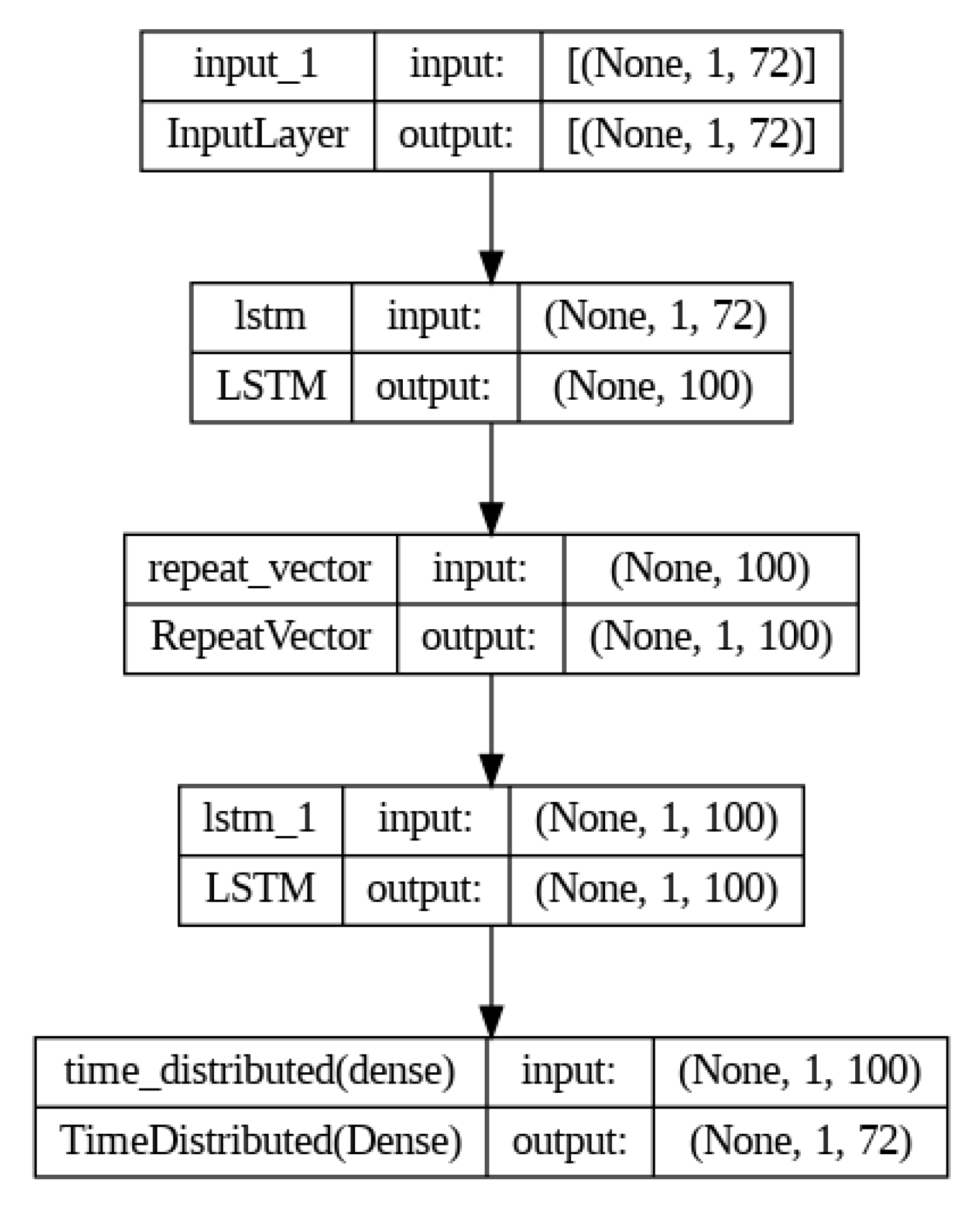
Figure 7.
Result of feature augmentation using the LSTM autoencoder.
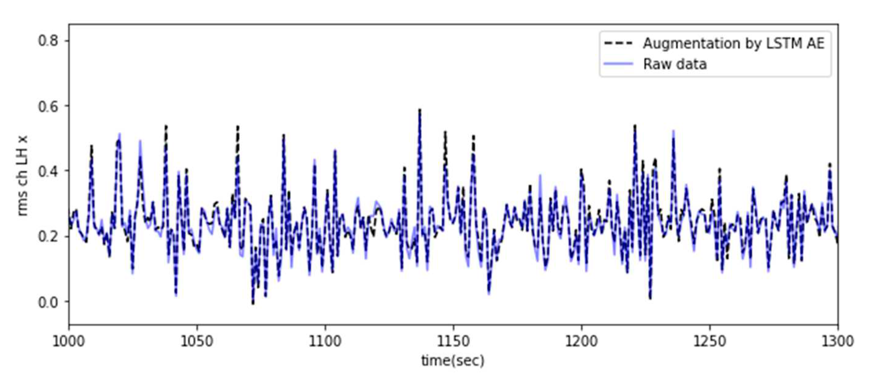
Figure 8.
Two kinds of tree growth (a) Level-wise growth, (b) Leaf-wise growth.
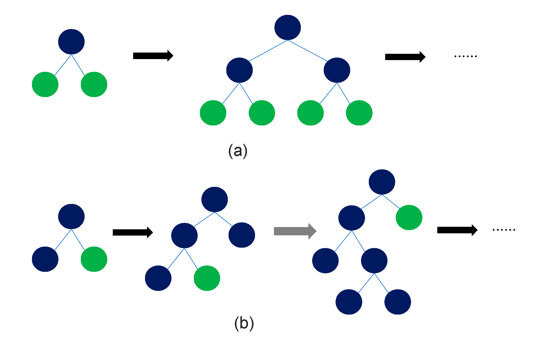
Figure 9.
Hyperparameters tuning result of the random forest and lightGBM.
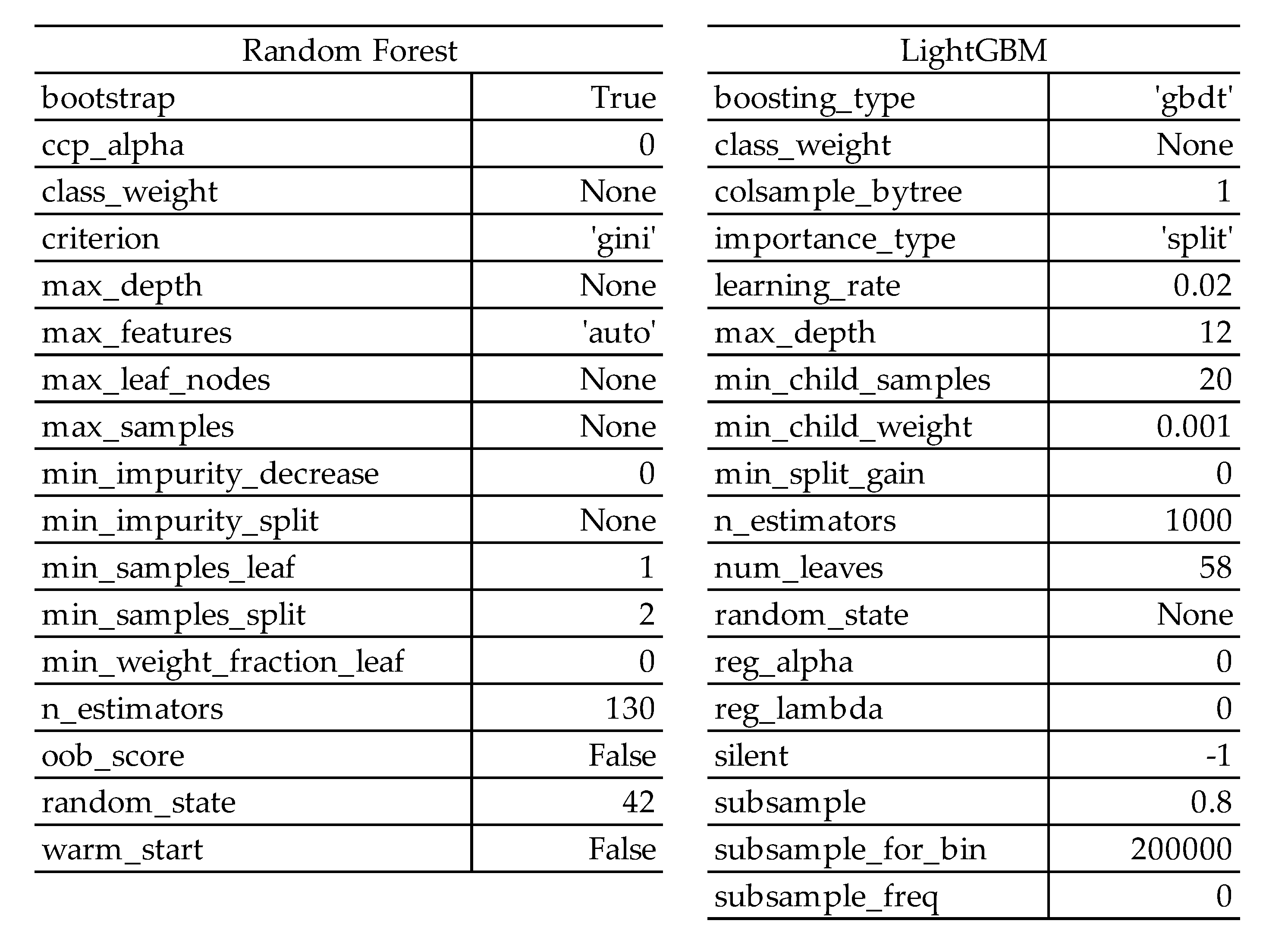
Figure 10.
Training and prediction.
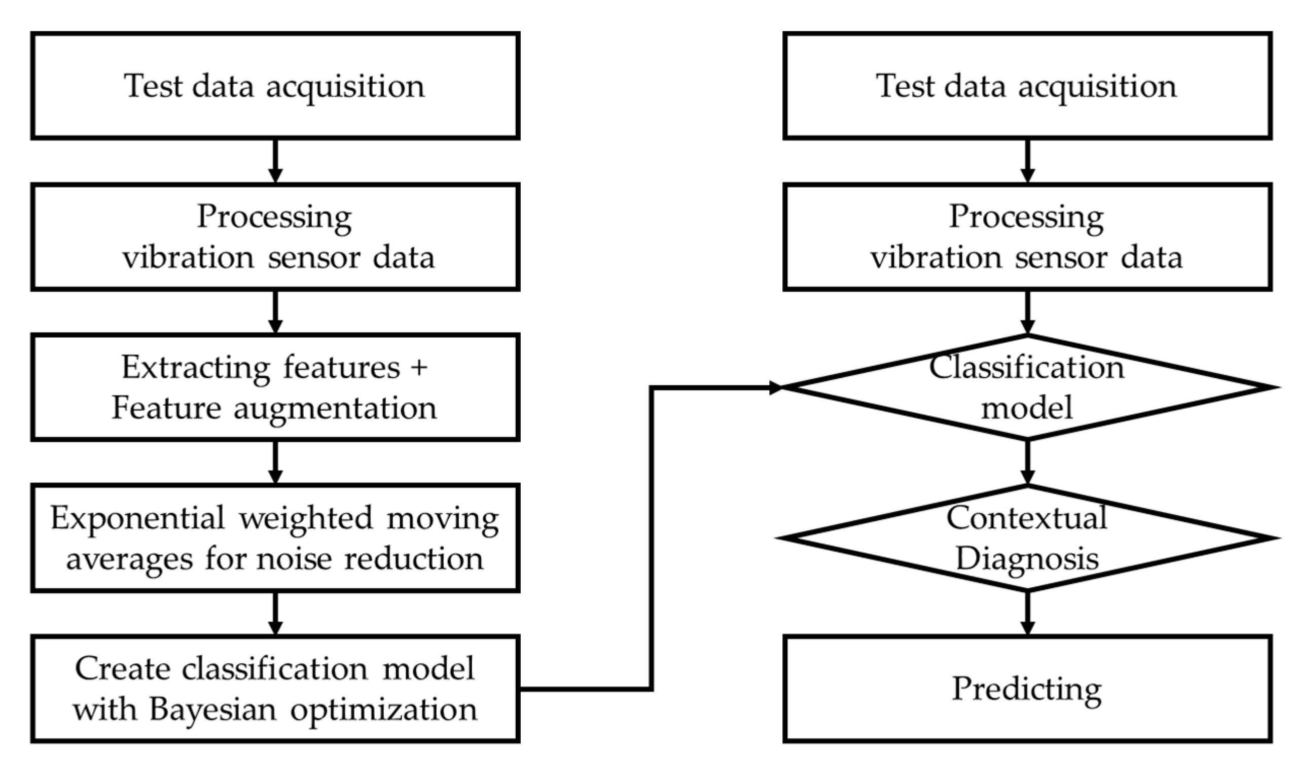
Figure 11.
Contextual diagnosis graph of light GBM (left: original, right: after moving average).
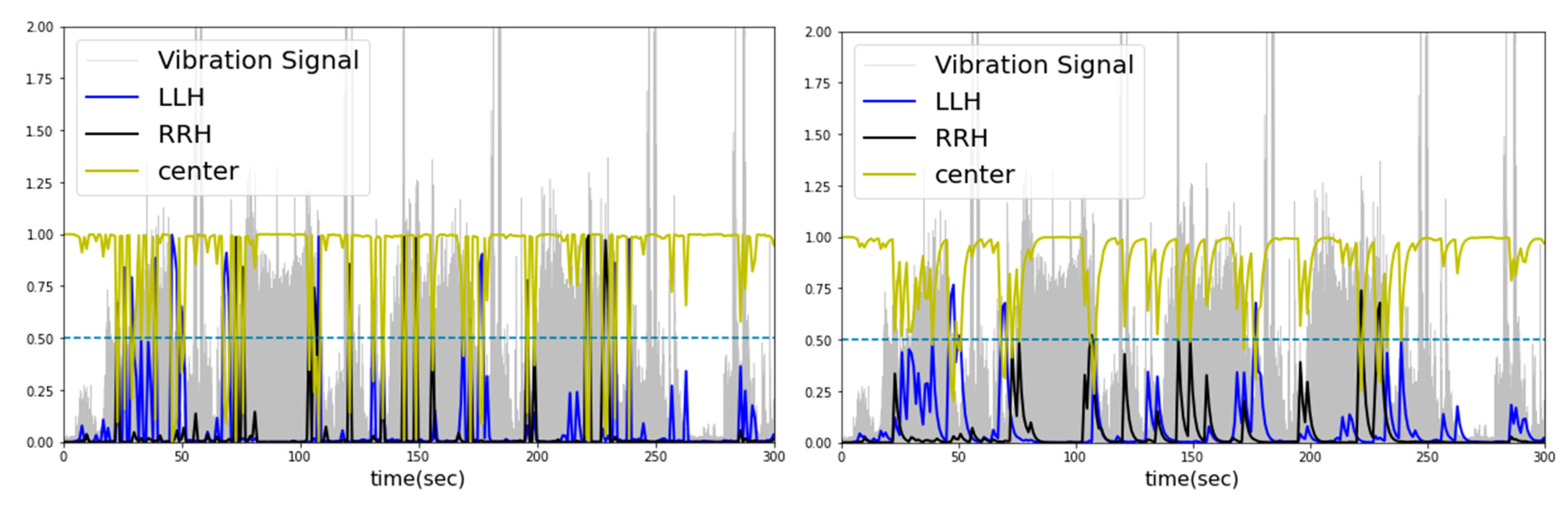
Figure 12.
Contextual diagnosis graph of random forest (left: original, right: after moving average).
Figure 12.
Contextual diagnosis graph of random forest (left: original, right: after moving average).
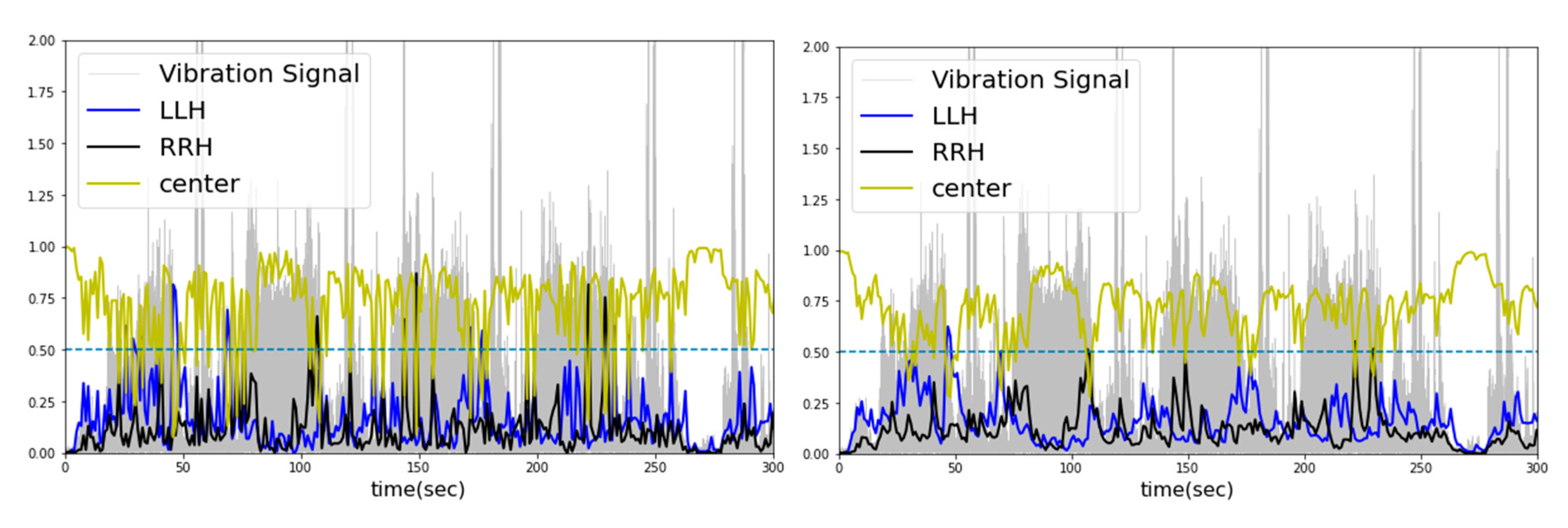
Figure 14.
Raw signal graph and STFT (Short-Time Fourier Transform) image of the measured sound data.
Figure 14.
Raw signal graph and STFT (Short-Time Fourier Transform) image of the measured sound data.
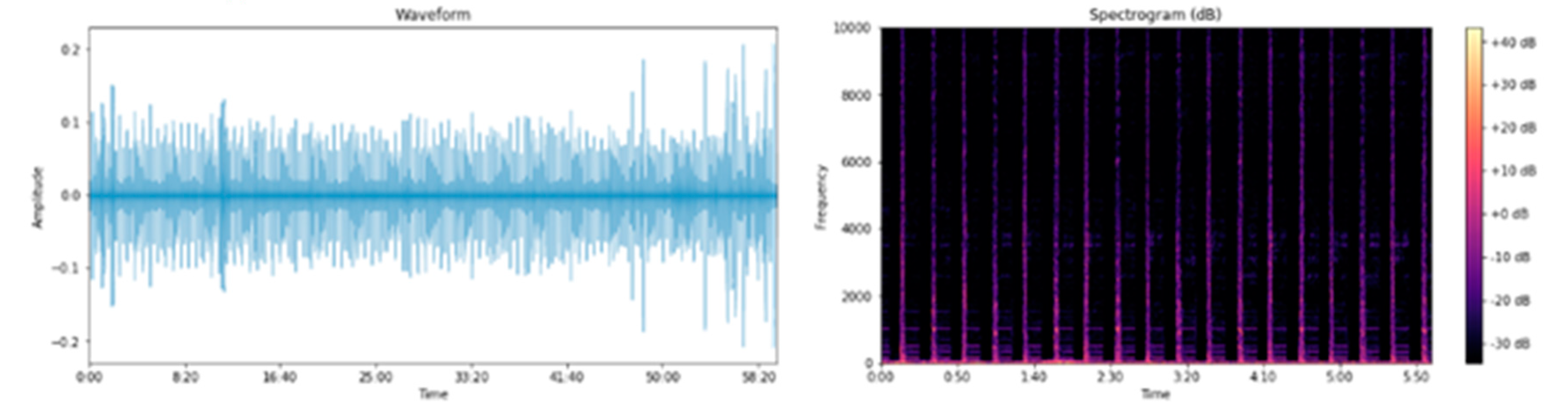
Figure 17.
Probability graph of logistic regression classifier.
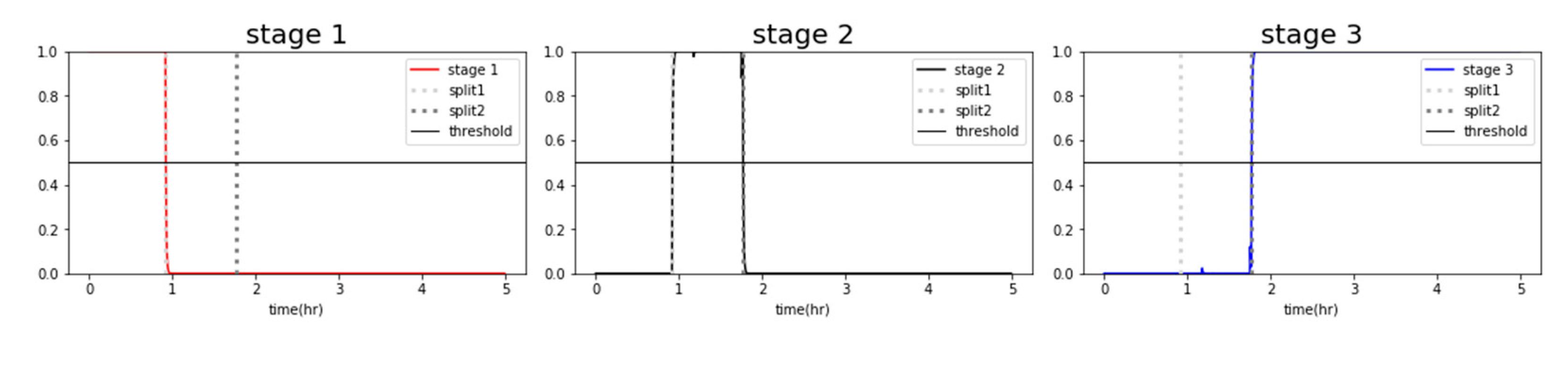
Figure 18.
Probability graph of the random forest classifier.
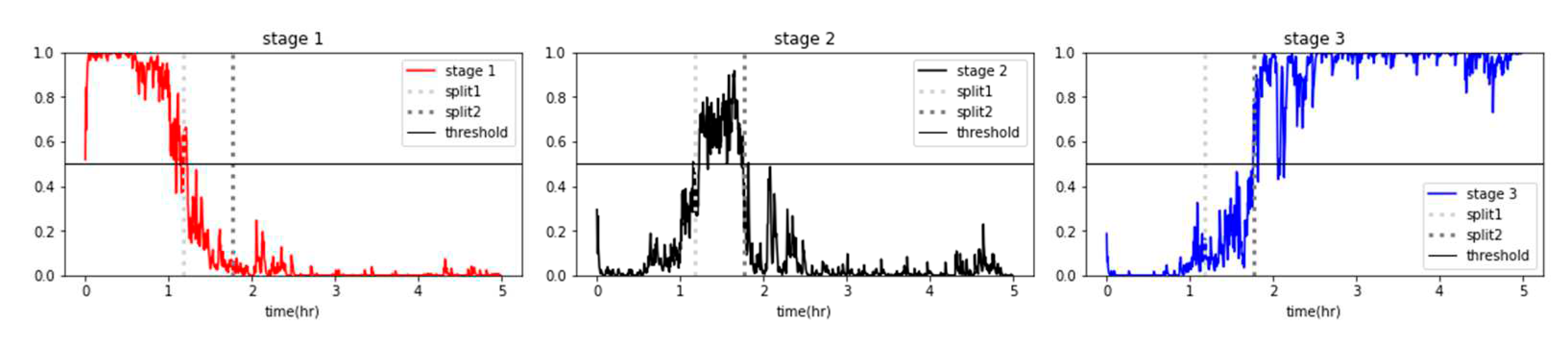
Figure 19.
Degradation graph of forklift using the average probability of a random forest classifier.
Figure 19.
Degradation graph of forklift using the average probability of a random forest classifier.
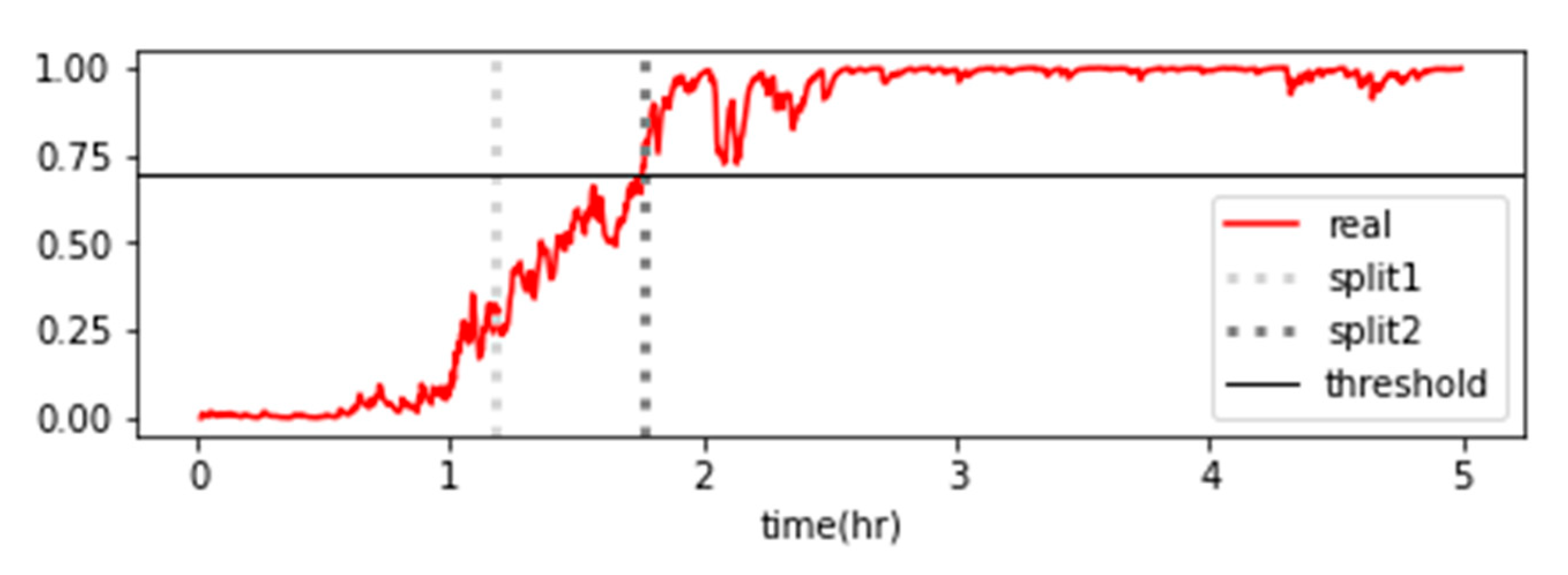
Table 1.
Description of feature (crest factor, shape factor, impulse factor, and margin factor).
| Crest factor | max/RMS |
| Shape factor | RMS/mean(abs) |
| Impulse factor | max/mean(abs) |
| Margin factor | max/mean(abs)2 |
Table 6.
Contextual diagnosis result.
| Before contextual diagnosis | After contextual diagnosis | ||||||
|---|---|---|---|---|---|---|---|
| time | Left(LLH) | Right(RRH) | Center | time | Left(LLH) | Right(RRH) | Center |
| 1 | 0.00112 | 0.00014 | 0.99874 | 1 | 0.00112 | 0.00014 | 0.99874 |
| 2 | 0.00305 | 0.00044 | 0.99651 | 2 | 0.00241 | 0.00034 | 0.99725 |
| 3 | 0.00239 | 0.00070 | 0.99691 | 3 | 0.00240 | 0.00055 | 0.99706 |
| 4 | 0.00103 | 0.00012 | 0.99885 | 4 | 0.00167 | 0.00032 | 0.99801 |
| 5 | 0.00117 | 0.00022 | 0.99862 | 5 | 0.00141 | 0.00027 | 0.99832 |
| 6 | 0.02492 | 0.00198 | 0.97311 | 6 | 0.01335 | 0.00113 | 0.98552 |
| 7 | 0.06715 | 0.01467 | 0.91818 | 7 | 0.04046 | 0.00795 | 0.95158 |
| 8 | 0.06500 | 0.00303 | 0.93197 | 8 | 0.05278 | 0.00548 | 0.94174 |
| 9 | 0.13749 | 0.01739 | 0.84512 | 9 | 0.09522 | 0.01145 | 0.89333 |
| 10 | 0.07009 | 0.01556 | 0.91436 | 10 | 0.08264 | 0.01351 | 0.90385 |
| . | … | … | … | . | … | … | … |
| . | … | … | … | . | … | … | … |
| . | … | … | … | . | … | … | … |
| m | … | … | … | m | … | … | … |
Table 7.
Case study result.
| case no. | dataset | machine learning model |
feature moving average window size | smoothing factor(α) | contextual diagnosis accuracy score (probability moving average window size) |
||
|---|---|---|---|---|---|---|---|
| 1sec | 2sec | 3sec | |||||
| case01 | raw feature | Random forest | 1 sec | 1.00 | 0.7522 | 0.8135 | 0.8950 |
| case02 | raw feature | Random forest | 2 sec | 0.67 | 0.8019 | 0.8622 | 0.9186 |
| case03 | raw feature | Random forest | 3 sec | 0.50 | 0.8347 | 0.8752 | 0.9274 |
| case04 | with lstm ae feature | Random forest | 1 sec | 1.00 | 0.7392 | 0.8047 | 0.8904 |
| case05 | with lstm ae feature | Random forest | 2 sec | 0.67 | 0.7846 | 0.8470 | 0.9094 |
| case06 | with lstm ae feature | Random forest | 3 sec | 0.50 | 0.8216 | 0.8713 | 0.9263 |
| case07 | with AWGN feature | Random forest | 1 sec | 1.00 | 0.7487 | 0.8238 | 0.9020 |
| case08 | with AWGN feature | Random forest | 2 sec | 0.67 | 0.7994 | 0.8601 | 0.9203 |
| case09 | with AWGN feature | Random forest | 3 sec | 0.50 | 0.8294 | 0.8819 | 0.9366 |
| case10 | with all feature | Random forest | 1 sec | 1.00 | 0.7487 | 0.8587 | 0.9362 |
| case11 | with all feature | Random forest | 2 sec | 0.67 | 0.8033 | 0.8897 | 0.9450 |
| case12 | with all feature | Random forest | 3 sec | 0.50 | 0.8305 | 0.9048 | 0.9563 |
| case13 | raw feature | lightGBM | 1 sec | 1.00 | 0.7659 | 0.8453 | 0.9295 |
| case14 | raw feature | lightGBM | 2 sec | 0.67 | 0.8223 | 0.8858 | 0.9496 |
| case15 | raw feature | lightGBM | 3 sec | 0.50 | 0.8646 | 0.9129 | 0.9637 |
| case16 | with lstm ae feature | lightGBM | 1 sec | 1.00 | 0.7621 | 0.8347 | 0.9098 |
| case17 | with lstm ae feature | lightGBM | 2 sec | 0.67 | 0.8160 | 0.8773 | 0.9369 |
| case18 | with lstm ae feature | lightGBM | 3 sec | 0.50 | 0.8488 | 0.9041 | 0.9521 |
| case19 | with AWGN feature | lightGBM | 1 sec | 1.00 | 0.7642 | 0.8421 | 0.9161 |
| case20 | with AWGN feature | lightGBM | 2 sec | 0.67 | 0.8379 | 0.8925 | 0.9485 |
| case21 | with AWGN feature | lightGBM | 3 sec | 0.50 | 0.8643 | 0.9122 | 0.9591 |
| case22 | with all feature | lightGBM | 1 sec | 1.00 | 0.7638 | 0.8389 | 0.9221 |
| case23 | with all feature | lightGBM | 2 sec | 0.67 | 0.8206 | 0.8883 | 0.9454 |
| case24 | with all feature | lightGBM | 3 sec | 0.50 | 0.8569 | 0.9115 | 0.9566 |
Table 8.
Stage labeling results of the sound data features using the CART (Classification and Regression Trees) algorithm.
Table 8.
Stage labeling results of the sound data features using the CART (Classification and Regression Trees) algorithm.
| feature | breakpoint 1 | breakpoint 2 |
|---|---|---|
| max | 0.892 | 1.764 |
| min | 0.925 | 1.775 |
| peak2 | 0.925 | 1.775 |
| skewness | 1.308 | 1.831 |
| Crest Factor | 1.353 | 1.708 |
| Shape Factor | 1.308 | 1.775 |
| Impulse Factor | 1.353 | 1.764 |
| Margin Factor | 1.353 | 1.775 |
| average | 1.177 | 1.771 |
Table 9.
Labeling and structure of a dataset.
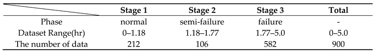
Table 10.
Validation result of stage classification.
| Model | Dataset | Accuracy | F1 Score | F1 Score |
|---|---|---|---|---|
| (weighted) | (macro) | |||
| Logistic Regression |
Case 1(vibration feature) | 0.9815 | 0.9814 | 0.9599 |
| Case 2(vibration+sound feature) | 0.9889 | 0.9891 | 0.9790 | |
| Random Forest |
Case 1(vibration feature) | 0.9519 | 0.9523 | 0.9116 |
| Case 2(vibration+sound feature) | 0.9556 | 0.9556 | 0.9220 |
Disclaimer/Publisher’s Note: The statements, opinions and data contained in all publications are solely those of the individual author(s) and contributor(s) and not of MDPI and/or the editor(s). MDPI and/or the editor(s) disclaim responsibility for any injury to people or property resulting from any ideas, methods, instructions or products referred to in the content. |
© 2023 by the authors. Licensee MDPI, Basel, Switzerland. This article is an open access article distributed under the terms and conditions of the Creative Commons Attribution (CC BY) license (http://creativecommons.org/licenses/by/4.0/).
Copyright: This open access article is published under a Creative Commons CC BY 4.0 license, which permit the free download, distribution, and reuse, provided that the author and preprint are cited in any reuse.


