
Submitted:
10 June 2023
Posted:
12 June 2023
You are already at the latest version
Abstract
During the last few years, several approaches have been proposed to improve early warning systems for reducing rock-fall risk. In this regard, this paper introduces a Deep learning-and (IoT) based Framework for Rock-fall Early Warning, devoted to reducing the rock-fall risk with high accuracy. In this framework, the prediction accuracy was augmented by eliminating the uncertainties and confusion plaguing the prediction model. In order to achieve augmented prediction accuracy, this framework fused the prediction model-based deep learning with a detection model-based Internet of Things. In order to determine the framework’s performance, this study adopted parameters, namely overall prediction performance measures, based on a confusion matrix and the ability to reduce the risk. The result indicates an increase in prediction model accuracy from 86% to 98.8%. In addition, a framework reduced the risk probability from (1.51 ×10⁻³) to (8.57 ×10⁻⁹). Our results indicate the framework’s high prediction accuracy; it also provides a robust decision-making process for delivering early warning and lowering the rock-fall risk probability.
Keywords:
rock-fall risk
; internet of things IoT
; deep learning
; early warning
1. Introduction
Rock-fall is a complex natural phenomenon that threatens humans and infrastructures in many mountain regions of the World. Because rock-fall events are random, reliable mechanisms for monitoring, predicting, and managing the geological risk due to rock-fall is still a challenging task. Many approaches have been used to model and assess rock-fall hazards in recent years. For example, literature [1] developed a hazard assessment model based on the frequency of rock falls, rock structure, and bounce height. By using a dynamic computational technique, the suggested model evaluated the risk of rock-fall and the quantification uncertainties. Quantitative models were also created to evaluate and control the danger of rock falls [2,3].
There is another technique to detect falling rocks, such as seismic signals detection. The literature reports many methods to track seismic waves produced by falling rocks, as geophysical sensors were developed to track the seismic signals caused by falling boulders and determine how the rock’s effect on the surface was estimated [4]. A micro-seismic approach was introduced to identify rock-fall occurrences in another investigation [5]. Although these methods are excellent in detecting rock-fall occurrences, doing so needs a large number of seismic sensors. Through the use of micro-electromechanical and micro-seismic networks, new methods to circumvent micro-seismic limits have been developed. Camera-based monitoring techniques have been recently used to monitor better and track fallen rocks in real time. A test version of an artificial intelligence camera was used to track and monitor falling rocks in real-time [8]. The camera has outperformed many technologies, even the micro-seismic networks, regarding to its capability to monitor many rocks simultaneously. The seismic and camera-based monitoring systems are used to identify falling rocks at the time of impact; nevertheless, they must be sufficiently effective to alert vehicles to the risk of rock-fall before it happens. Unfortunately, this technology responds to events after causing severe damage to the road and pedestrians. In order to get around the limitations of monitoring approaches, rock-fall occurrences must be predicted. Recently, excellent models to forecast rock-fall dangers have been created using machine learning technology. Various machine-learning techniques, including logistic regression, have been utilized for predicting rock falls [9,10] and support vector machines (SVM) [11,12]. Another approach [13] developed a tool for predicting the spatiotemporal distribution of rock-fall using artificial neural networks and linear regression. The rock-fall risk was assessed using several approaches, such as a (Hybrid Early Warning System for Rock-Fall Risks Reduction) [14]; this system uses three models to predict the likelihood of rock falls the logistic regression model, the computer vision model, and the hybrid risk reduction model, which also provides early warning and hazard level classification. Because the model was created using insufficient historical data about a particular location, the current prediction approaches are ineffective at reducing the rock-fall risk in real-time.
Although this system contributed to reducing the risk of rock falls, the prediction process still needs to be more accurate and uncertain because it inherited previous models’ limitations. In order to get over the constraints of all earlier models, offering an accurate prediction is necessary.
This study proposed a framework to reduce the rock-fall risk. The primary purpose of this framework is to augment the prediction accuracy by eliminating the uncertainties and confusion that plague the prediction model. In order to achieve a prediction accuracy augmentation, four different techniques were integrated, detection model-based (Computer Vision and Micro-seismic wave), prediction-based (Deep Learning model), Internet of Things network (IoT), and (Decision Make Algorithm).
Finally, The following are the key contributions of this study:
- We propose IoT based framework for rock fall Early Warning.
- We created a (Deep learning model) to predict the likelihood of rock-fall events.
- We created a detection model-based (Micro-seismic wave and Computer Vision).
- We have augmented the accuracy of a prediction model by fusing the detection model with a prediction model.
- We developed a (Decision Make Algorithm).
- We provide a baseline methodology and a prediction accuracy benchmark for future related works.
2. Study Area and Problems
The study targeted two sites in southern Saudi Arabia along the( Sarawat mountain), constituting a natural obstacle to communication between cities and population centers above the mountains and those scattered in the plains and valleys [15]. The first site (Aqabat Shaar) a located on the road linking the city of Abha and Mahayel Asir, and this obstacle extends a length of 14 km on mountain ranges with a height of 2160 meters. The second site (Aqabat Dhala) a located on the road linking the cities of Abha and Jazan. This obstacle extends 11 km along a steep mountain at 2220 meters high. These two sites have many bends and tunnels, crowded with high traffic intensity, which increases the possibility of exposed cars at the moment of a rock fall.
One of the most important reasons that lead to the fall of rocks in this area is the constant rainfall throughout the summer on the mountain range, which causes an absolute nightmare for the passers-by of the (Aqabat Shaar )and (Dhala). It is stable and becomes suitable for the fall of rock masses. Also, one of the causes of rock fall in this area is the nature of the rock formation in some locations, where it consists of large rocky blocks interspersed with rocky rubble in addition to other areas permeated by a limestone layer. This formation made it weak in resistance to natural factors. The difference in temperatures between night and day characterizes these areas. These temperature differences, in addition to ground movements, cause rock stress, which leads to cracks. This crack expands with time, and rainwater retracts into the cracks, causing pressure on the rocks, which reduces cohesion’s strength and results in successive rock slides [16].
The construction work in the area led to the emergence of edges with sharp sloping angles, which reduced the gravity of the rock masses and made it easier to roll them downwards, increasing the possibility of rocks falling at any moment.
3. Data acquisition
3.1. Data Collection and Preparation
The historical data of the rock-fall events, in addition to meteorological data were collected in a period from January 2015 to August 2021. Different sources as, KSA Civil Defense, Geological Hazards Research Center were used as data source. This period was divided into 2040 samples, which included 415 rock-fall events. During the initial filtering of the data, three non-dependent variables (slope angle, Rainfall, and temperature variation) and one dependent variable (rock-fall event) were selected. A training data set of 70% (1428 samples) and a test data set of 30% (612 samples)were created from the rock-fall inventory data in order to training and testing the model.
3.2. The rockfall condition factors
The decision to use rock-fall conditioning factors directly affects mathematical models’ accuracy. [17,18]. This study utilized three rock-fall conditioning factors, hydrological (rainfall), topographic (slope angle), and weather-related. (Temperature variation) [19].
In considerable rock-fall events, rainfall directly affects the movement and rolling of rocks [20]. The rock fall events are directly proportional to the slope angle of the mountain. The higher the slope angle, lead to less rock stability [21]. The difference in temperature between day and night exposed rocks to expansion and contraction, which led to cracks in the rocks [22].

Table 1.
Rock-fall conditioning factors.
| Type | Factor | Unit | Factor Class |
|---|---|---|---|
| Topographic | slope angle | degree | ( range 20 - 60 ) |
| Hydrological | rain full | mmh-1 | ( range 0 - 46) |
| Weather | temperature variation | co | ( range 0 - 21 ) |
4. Methodology
4.1. Rock-Fall Early Warning Framework Design
This section presents a framework-based Internet of Things (IoT) for Rock-Fall Early Warning. Figure 1 shows our proposed framework for detecting and predicting rock-fall incidents. The framework consists of five layers: field layer, edge layer, fog computing layer, cloud computing layer, and data presentation layer.
4.1.1. Things layer
Includes the actual sensors to measure the physical parameters of interest; these include rainfall, air temperature, air humidity, a seismic sensor for detecting seismic waves, and a camera for rock movement detection; the field layer also expanded to accommodate intelligent voice module and light panel to run out the early warning action.
4.1.2. Edge Computing layer
In order to decrease network traffic and energy consumption, the edge nodes gather input from the sensors and conduct data and image processing algorithms. The main goal is to locally generate fundamental model properties of the specific process, which pass on to the fog computing compactly. Also, execute commands incoming from higher-level systems to deliver an early warning action and make local decisions, thus preventing upper-layer latency.
4.1.3. Fog Computing layer
It bridges the gap between the cloud and edge nodes by enabling computations such as rock-fall monitoring, rock-fall prediction, deep learning model, rock-fall risk Assessment, networking, data management, and decision making. Blynk cloud was used in this study (Blynk cloud); it’s a comprehensive software package needed to deploy and remotely manage linked electrical devices at any size, from small-scale home IoT projects to millions of commercially connected items.
4.1.4. Cloud computing layer
The cloud was chosen to provide communication service by streaming data between the fog computing and data presentation layers and providing a medium for data storage. The Blynk utilizes HTTPS (API) to report telemetry and regularly fetch DataStream. Additionally, it offers open-source hardware libraries so that any device may connect to Blynk Cloud.
4.1.5. Data presentation layer
Concerned with the software systems that convey the data analysis results to end-users or decision-makers. In this study, Web and Mobile app dashboards are used to present the early warning alarm in the case of event detection, in addition to affording the system administrator access privileges and decision-makers.
4.2. Rock-fall detection model
This study obtained a robust rock-fall detection model by gathering two detection processes. First, computer vision algorithm was used to detect rock-fall event. Secondly, seismic wave sensors were used to detect the vibrations from rock cracking or falling.
4.2.1. Rock-fall detection-based computer vision
The computer vision algorithms detect the rock-fall events in three steps, as in Figure 6. filtering the image frame, background subtraction, and performing frame manipulation as in Figure 6. In the first step, the (Blurring Gaussian Filter) was used to filter out the noise from the captured images. Secondly, the moving rocks were detected from the video frame sequence. Due to weather conditions and daytime, the video frame sequence suffers from background illumination variations, so the (Adaptive Gaussian Mixture Model) was used to overcome this problem.
The model treats each pixel as a composite of Gaussians before learning the image’s backdrop and categorizing each pixel as background or foreground. The background model is represented by Equation 1.
where represents the estimated background, is the grayscale of the pixel value at time t, M is the number of the Gaussian components, represents the training set, the weight indicates how much of the data is part of the m component of the GMM, is estimated means, I represents an identity matrix, and is the estimates variances.
The (Bayesian) was used to classify pixels as background or foreground from moving rocks video frame [23]. The frame manipulation was used to overcome imperfections in the segmentation process.
4.2.2. Rock-fall Detection based micro-seismic wave
The seismic wave is generated in two cases, at the moment rocks crack or when rocks fall. Thus, the seismic wave sensor can be used to detect rock fall events. This study characterized the micro-seismic wave by its frequency component, classified into three frequency domains. A significant frequency spectrum band between 100 and 1000 Hz was present in the first domain. These signals are generated several hours prior to the rock’s fall. The second domain is in the higher frequency band between 500 and 1000 Hz.
The third domain is in the lower frequency spectrum, 100 to 500 Hz. These signals precede the rockfall event by a few moments. The relationship between Rock-fall incidents and seismic wave frequency domains was quantified using the spectral amplitudes ratio (R). The spectral amplitude ratio (R) is calculated according to Equation(2) [24].
where AMAX(100Hz−500Hz) is the maximum amplitude of the frequency spectrum 100 Hz to 500 Hz, AMAX (500Hz−1000Hz) is the maximum amplitude of the frequency spectrum 500 Hz to 1000 Hz. The average amplitude ratio R for all frequency domains is shown in Table 2.
4.3. Rock-fall Prediction Model
Due to the randomness of a rock-fall occurrence, the function of the rock-fall event probability P = fx(r, s, t) is uncertain; therefore, mapping the relationship of the rock-fall possibility P, the slope angle s, the rain-full r, and the temperature variation t cannot be strictly described. To solve the uncertainty of the mapping function, the BP (backpack) artificial neural network can learn the relationships between the input and the output of the corresponding procedure by analyzing the sample data and adopting a model to give the expected output value when given the input value [25].
4.3.1. Deep Learning Model.
In this paper, we proposed a deep learning model for a rock-fall occurrence prediction. It is one of the machine learning process. It is a complex mathematical model that simulates the biological neuron structure and self-learning function; It uses mathematical methods that are based on the idea of linked layers of nodes. [26]. As seen in Figure 4, it has an output layer, three hidden layers, and a three-parameter input layer.
Figure 3.
Deep learning model design.
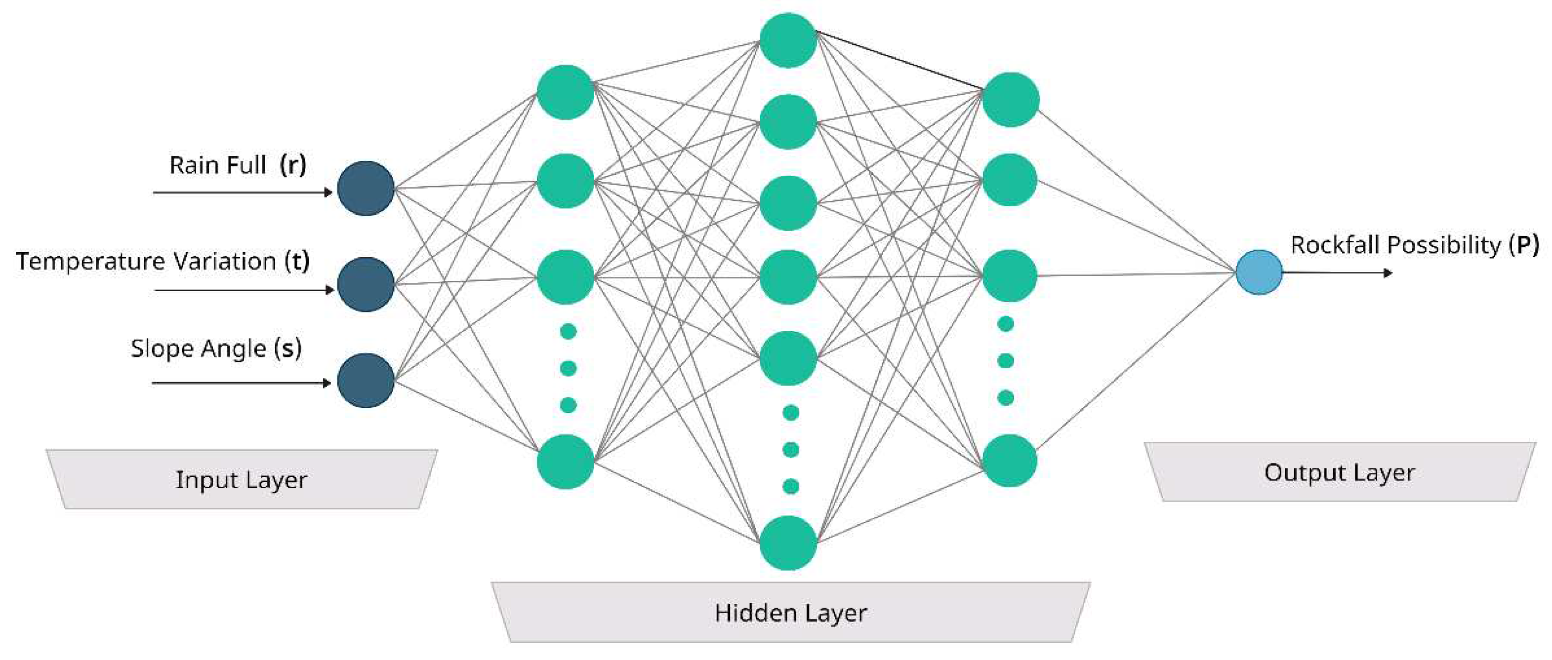
As shown in Figure 4, each node in this neural network is a neuron, and each neuron has six major components, including inputs (xi), biases (bj), weights (wij), sum functions (uj), activation functions (f), and outputs (yj). The information from neurons or the outside world that is used as a decision variable is referred to as an input. Weights are values that translate how the influence of inputs on one another. The sum function (Equation (3)) is an operation that takes into account a bias value and reflects the impacts of inputs and weights[27].
where:
i is the ith input neuron
j is the jth output neuron
n is number of elements in the ith input vector.
bj is the bias value (also known as the activation threshold) connected to the jth node.
According to the equation in Equation (4), the activation function is in charge of converting the node’s summed weighted input into the activation of the node or output for that input.
where yj represents the output of the jth neuron, controls the slope of the rectified linear activation function, and is typically equal to 1.
4.3.2. Training Methods
The SciKit-Learn neural network package was used to create the neural network models that were used in this study. The model was generated with three hidden layers. In our method, the training process used 70% of the entire data, while the validation process used 30% of the remaining data. The training process was operated using the multilayer perceptron (MLP). The MLP was chosen because it provides quick predictions after training. It utilizes a supervised learning technique called backpropagation for training with the rectifier linear unit (ReLU). The learning algorithm performs backpropagation, which calculates the correct gradient for nonlinear multilayer networks to reduce errors (the gap between prediction and actual values)[28].
In this study, a gradient descent method was used as an optimization model. This method is to update the variables iteratively in the (opposite) direction of the gradients of the objective function. Equation (5) performs the gradient descent algorithm. It updates the weight and bias parameters iteratively in the negative gradient direction to minimize the loss function f(θ).
where α is a learning rate, f(θ) is a loss function, θj is the weight or bias parameter, which we need to update.
4.3.3. Model Performance Validation
In this section, the overall model performance (recall, specificity, precision, F1-Score, and accuracy), as well as the mean squared error (MSE) and area under a receiver operating characteristic (ROC) curve (AUC), were used to validate the model’s ability to distinguish between the occurrence of a rock-fall and a non-rock-fall event. The system performance was calculated using the confusion matrix. [29]. The first metric is recall, which referred to as sensitivity or the true positive rate. The following calculation measures how well the model predicted the rock-fall event:
The second metric, Specificity, is used to assess a system’s capacity to verify the absence of a rock-fall event, which is described as
The third metric is precision, it is used to determine how many samples really fall into the positive class out of all those that the model projected would.
The fourth metric is F1 score, is used as a model’s predictively assessment. The F1 score is derived by combining the accuracy score and the recall score of a model, and its definition is as follows:
The fifth metric is accuracy, which is a reflection of how accurately the system can identify the rock-fall event, its defined as follows:
Whereas true positive (TP) indicates that all events were indeed discovered, false negative (FN) indicates that some events took place but went undetected, and true negative (TN) indicates that no events took place. A false positive (FP) event is absent, yet the system records it as present. The system reports an absent event.
Equation (11) uses the Mean Squared Error (MSE) to calculate the average squared difference between the values of real and predicted data points in order to quantify the degree of error in the learning model.
where n is the total number of data points in the dataset, Yi is the actual data point values, and i is the projected data point values. The overall performance of a prediction is measured using the area under a receiver operating characteristic (ROC) curve (AUC), which is based on a confusion matrix.
4.4. Rock-fall Risk Assessment
The likelihood that a rock-fall event will occur at a specific location and at a specified time and impose a specific level of damage to roads, automobiles, and pedestrians was characterized as rock-fall risk. Then the risk is calculated in terms of the temporal and spatial information on the effect of precipitation. Based on the possibility that cars are available in a certain position and time period affected by rocks falling, the temporal-spatial probability and susceptibility were determined [30]. Equation (12) shows the risk probability’s value.
where P(Risk) denotes the likelihood that a rock fall incident will occur within a given hour and fr denotes the frequency of rock falls. The possibility that a rock will fall and impact the car is P(r). The susceptibility of the vehicle to rock-fall occurrences, or V(u), has two possible values: 1 if the rock actually hits the car, and 0 if it doesn’t. The likelihood that automobiles will be accessible at a particular location and time is known as P(S:T). There is (temporal-spatial probability) that a car traveling the entire path will be impacted at the moment of impact. It is determined using Equation (13) [31].
where Nv is the average daily number of vehicles, Lv is the average length of a vehicle in meters, and Vv is the average speed of a vehicle in kilometers per hour..
4.5. Rock-fall Prediction Model Augmentation
The prediction made by the Deep Learning model is subject to noise, model errors, and uncertainty [32]. Therefore, it is highly desired for any AI-based system to represent uncertainty in a reliable manner. In this part of the article, the prediction model had been enhanced by increasing the overall level of model accuracy so that a precise decision could be made to reduce the chance of a rock fall.
For our proposed model, noise in data and inadequate knowledge lead to uncertainty in data; subsequently, The naturally uncertain nature of the data is modeled by the predictions, making it irreducible. In this study, to address this problem, a new method was proposed to decrease the uncertainty by diminishing Two instances of confusion: situations of certain events occurring but not being identified as false negatives (FN) and cases of some events occurring but not being recognized as false positives (FP).
The augmented rock-fall prediction probability P(J), obtained by applying (the union of not mutually exclusive probabilities theory), between the probability of the rock-fall risk according to the detection models P(D), as well as the possibility of a rock fall according to the prediction models. P(p), The procedure of deriving the joint rock-fall probabilities using detection and prediction models is depicted in (Figure 5).
The rock-fall probability of the detection models calculated from the, micro-seismic detection model and computer vision detection model, then the joint probability is calculated as in Equation (14).
where P(D) is the rock-fall probability of the detection models, P(S ∪ V) is the union probability, P(S) is the rock-fall probability determined by the micro-seismic detection, P(V) is the rock-fall probability determined by the computer vision detection model, P)S ∩ V) is the probability of P(S) and, P(V) are mutually exclusive occur. In this study P(S) was determined from the spectral amplitudes Ratio (R) of the micro-seismic event, as in Equation (15).
where R is the spectral amplitudes ratio of a micro-seismic event, it takes the values from )1.5±0.08) to (7.1±0.68), as mentioned in Section (4.2), RMAX is the ratio of the spectral amplitude when the rock-fall occurrence is confirmed, and its value is equal to (7.78). The P(V) value is 0 in case of no rock fall is detected, and it is valued is 1 in case of rock-fall is detected. By Substituting the values of the probabilities into equation 6, we get Equation 16
The rock-fall occurrence probability (P*) which obtained from the prediction model (Artificial Neural Network) was used to determine the rock-fall risk probability. Finally, the augmented rock-fall prediction probability P(j) was calculated by joint the rock-fall probability of the detection models P(D) with the rock-fall risk probability of the prediction models P(P), Equation (17).
The overall accuracy of the augmented model can be obtained by Equation 18.
where Au is the augmented model accuracy, and δ is the uncertainty decreasing factor.
Ad is the average accuracy of the detection model.
4.6. Rock-fall Risk Reduction Process
The risk reduction process is carried out by preventing cars and pedestrians from entering the vulnerable area. This study used an early warning to prevent cars from entering a hazard zone. The likelihood that vehicles would not enter the danger zone after receiving the early warning signal at the time of the incident was used to determine the risk reduction [33]. In this study, the value of a risk reduction was calculated using the risk reduction probability, which includes the system reliability, the average number of cars, and the likelihood of vehicle response as in Equation (20).
where P(R) refers to the possibility that the risk will be reduced, P(rs) refers to the probability that a given vehicle will not reach the affected road segment after getting the warning signal, Nv refers to the average number of vehicles, and Au refers to the overall accuracy of the enhanced model. The value of P(re) is determined by applying Equation (21):
×Nv ×P(rs)
Based on the physical force distance, response time, and brake contact distance, the overall stopping distance was calculated. The safe distance is determined by the reaction time of the vehicle driver. The reaction time of the driver vary randomly in range between 0.4 and 2 seconds. The Physical Force Distance can be calculated by dividing the vehicle’s speed by the amount of time it takes for the brakes to react. When its acceleration of 10 m/s2 is implied [34].
4.7. Decision Make Algorithm
This algorithm was developed to make the appropriate decision about reducing the rock-fall risk. It fusion the outputs of the rock-fall prediction model (deep learning model) with the outputs of (the detection model) in order to obtain the augmented prediction, as well as calculating the risk of a rockfall, categorizing it into three levels, and creating a warning strategy to handle a severe hazard situation. The subsequent steps demonstrate how the proposed (Algorithm 1) utilizes and controls a rock-fall danger level.
| Algorithm 1 was performed in order to figure out the rock-fall risk, identify the risk level, and carry out the rock-fall risk reduction process. |
|
The first step: Gathering information with the things layer Read Rainfall by (Rain sensors) Read temperature by (temperature sensors) Read (IoT camera) video frames Read seismic waves by (seismic sensor) The second step: Detection of falling rocks in accordance to Equation (1) The third step: Determine the rock-fall occurrence probability(P) in accordance to Deep Learning model The fourth step: Compute the total rock-fall risk probability P(j) in accordance to Equation (17) The fifth step: Classifying the hazard in to three levels: When is greater than or equal to ( ) then hazard in unacceptable level. When is greater than and less than ( ) then hazard in tolerable level. When is less than or equal to ( ) then hazard in acceptable level. The sixth step: performing the risk reduction action Reducing the risk of rock falls by sounding and lighting warnings Turn on the (Red light + sound), when the hazard at unacceptable level. Turn on the (Yellow light), when the hazard at tolerable level. Turn on the (Green light), when the hazard at acceptable level. The seventh step: Return to first step. |
5. Results and Discussion
The research, findings, and framework discussion were presented in this section. The findings of the experiment provide demonstration for three different terms. First is the Deep-Learning model validation. First comes the validation of the deep learning model. The second is a risk assessment for rock falls. The assessment of the risk reduction comes last.
5.1 Deep Learning Model Validation
Performance metrics were obtained based on the four possibilities from the con-fusion matrix of TP, TN, FP, and FN, and were used to validate the proposed deep learning model (Table 3). These metrics included specificity, accuracy, precision, F1-Score, and area under a receiver operating characteristic (ROC) curve (AUC) metrics. In addition to Mean Squared Error (MSE).
A report on the deep learning model for the 612 testing sample obtained through the confusion matrix (Table 3). It shows that the actual detected events(TP) were 222, the number of events that occurred but were not detected(FN) was 35, the number of events that did not occur and the system generated an absence event report(TN) was 304, and the number of events was absent. However, the system reported it as present(FP) is 51. Additionally, the outcome demonstrates an ability to ignore fake occurrences, with an average specificity of 85.6%. The accuracy of 86% reflects the percentage of times a model produced a prediction throughout the entirety of the dataset.
The classification report (Table 4) shows the validation data average recall (sensitivity) for the both class (rock-fall even not occur 0) and (rock-fall even occurs 1) is 86%. That means, at the lowest sensitivity levels, only 14% of the rock-fall occurrences were improperly recognized. The average precision of 85% shows the amount of the positive predictions made by the model were correct. The average F1-Score is 86%.
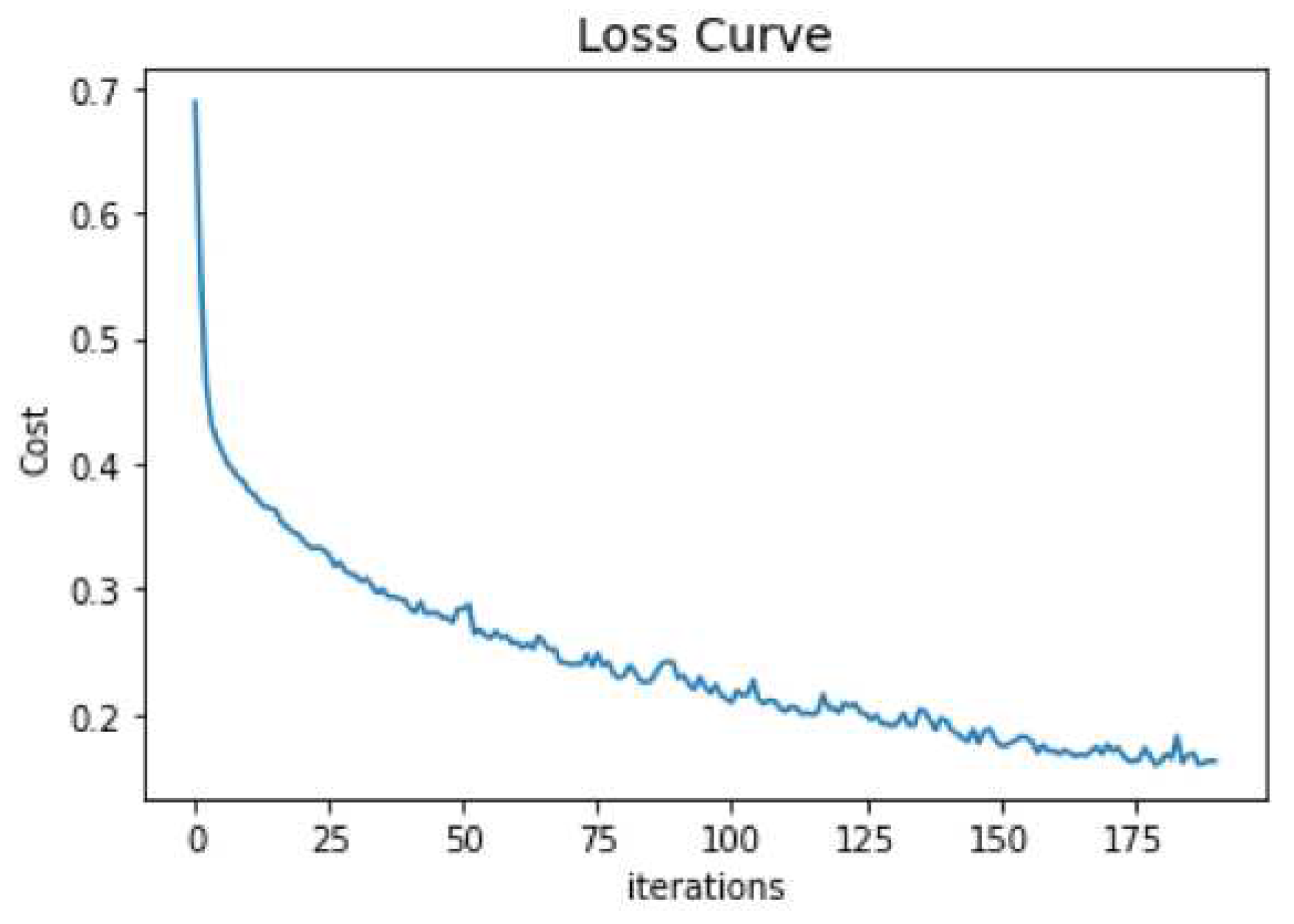
The deep learning model’s loss curve for 200 iterations is shown in Figure 6. In contrast, during the neural network training session, the cost value drops with each iteration. As a result, reflecting the performance of the learning through time. Finally, the cost value eventually dropped to less than 0.14 points, which is regarded as an acceptable Mean Squared Error (MSE) score.
Figure 6.
The Mean Squared Error (MSE) curve.
The ROC curve shown in Figure 7 demonstrates the model’s accuracy in predicting the occurrence of rock falls. The area under the ROC curve (AUC) value has reached 0.946.
5.2. Rock-fall risk assessment result
The method outlined in Section 4.4 (Equation 12) of this study was applied to calculate the Rock-fall Risk Probability. The Python environment was used as a simulation tool The settings and configurations used for the simulation are listed in (Table 5).
The findings indicate that the values for the highest and lowest rock-fall risk probability were, respectively (1.51 ×10⁻³) and (7.98 ×10⁻⁶). Moreover, the relationship between the local time and the rock-fall risk probability (Figure 8) shows that the high-risk probabilities are concentrated in the local time period between 12 pm and 18 pm.
In order to classify the risk values into three levels, The outcomes were compared to the triangle of safety-critical regulation and management thresholds, which is shown in Figure 9 (ALARP)[35]. The result shows that the risk probability values were spread among all (ALARP) levels. 29.1% of values are unacceptable, and the remaining risk values are divided between acceptable and tolerable levels by 16.6% and 54.2%, respectively.
5.3. Rock-fall risk reduction
The risk reduction was obtained by applying a decision-making algorithm. Figure 10 shows that the Rock-fall risk probability was decreased to values ranging from (8.57 ×10⁻⁹) to (8.21 ×10⁻⁷). When these values were compared with (ALARP) levels, we found that all values were less than (1 ×10⁻⁶), and therefore all values were Located at acceptable levels.
Table 6.
Rock-fall Risk probability before and after reduction.
| Rock-fall Risk Probability | Minimum | Maximum |
|---|---|---|
| Before Reduction | 7.98 ×10⁻⁶ | 1.51 ×10⁻³ |
| After Reduction | 8.57 ×10⁻⁹ | 8.21 ×10⁻⁷ |
The overall accuracy of the augmented model was obtained by substituting the detection model’s average accuracy into Equation (19). We found that the overall accuracy after augmentation increased from 86% to 98.8%, as in (Table 7). This result confirms the effectiveness of the augmentation in raising the model accuracy and reducing the confusion associated with the prediction process.
6. Conclusions
In this study, an early warning framework was developed to reduce the risk of rock falls. First, 2040 samples of historical rock-fall events data were gathered from various sources, and randomly split into two groups, with 70% going for deep-learning model training and 30% going for model validation. Next, the model prediction accuracy was augmented using a real-time rock-fall detection model based on (IoT) and computer vision. Finally, the decision-making algorithm assesses the risk of a rockfall, categorizing it into three levels, and producing a warning reaction to handle the critical hazard situation.
This study utilized parameters and overall prediction performance measures based on a confusion matrix to compare the performance of the model before and after augmentation. The results showed that the models had acceptable performance. The results show that the overall model accuracy before augmentation was 86%, which became 98.8%after the augmentation. Additionally, as shown in (Table 6), a framework can lower the risk probability from (1.51 ×10⁻³ ) to (8.57 ×10⁻⁹).
By comparing our new augmented model with our model in a previous study [14] based on performance and the ability to reduce the risk of rock fall, we discovered that the new proposed model’s prediction accuracy was 98.8%. In comparison, the previous study’s accuracy was 97.9%. In addition, the new model reduced the risk probability to (8.57 ×10⁻⁹), while the previous study reduced the risk to (1.13 ×10⁻⁸). This result indicates that although the previous model had acceptable performance, the augmented model outperformed this model. It can be considered a promising technique for predicting and reducing a rock-fall risk.
In future studies, we suggest enhancing the real-time rock-fall detection process by increasing the number of seismic sensors to achieve a higher detection accuracy and enhancing the current DL prediction model accuracy by adding more rock-fall conditioning factors.
Author Contributions
Conceptualization, M.A. and H.D.; methodology, M.A.; software, H.D.; validation, M.A., H.D., and T.A.; formal analysis, M.A.; investigation, M.B.; resources, H.A. and M.I.; data curation, A.H.; writing—original draft preparation, M.A.; writing—review and editing, H.D. and A.M; visualization, M.M.; supervision, M.A.; project administration, M.A.; funding acquisition, M.A. All authors have read and agreed to the published version of the manuscript.
Funding
Please add: This research received no external funding.
Institutional Review Board Statement
Not applicable.
Informed Consent Statement
Not applicable.
Data Availability Statement
Not applicable.
Acknowledgments
The authors extend their appreciation to the Deanship of Scientific Research at King Khalid University for funding this work through Large Group (Project under grant number (RGP.2/320/44)).
Conflicts of Interest
The authors declare no conflict of interest.
References
- Budetta, P. Assessment of rockfall risk along roads. Nat. Hazards Earth Syst. Sci. 2004, 4, 71–81. [Google Scholar] [CrossRef]
- Luciano, P. Quantitative risk assessment of rockfall hazard in the amalfi coastal road. Available online: https://upcommons.upc.edu/handle/2099.1/4937 (accessed on 1 February 2021).
- Sun, S.-Q.; Li, L.-P.; Li, S.-C.; Zhang, Q.-Q.; Hu, C. Rockfall Hazard Assessment onWangxia Rock Mass inWushan (Chongqing,China). Geotech. Geol. Eng. 2017, 35, 1895–1905. [Google Scholar] [CrossRef]
- Steiakakis, C.; Partsinevelos, P.; Tripolitsiotis, A. ; Agioutantis, Z; Mertikas, S., Ed.; Vlahou, G. Design and System Architecture of the GEOIM Rockfall Monitoring System. In 5th Interdisciplinary Workshop on Rockfall Protection-RocExs; RocExs: Lecco, Italy, 2014. [Google Scholar]
- Collins, D.S.; Toya, Y.; Hosseini, Z.; Trifu, C.I. Real Time Detection of Rock Fall Events Using a Microseismic Railway Monitoring System; Geohazards: Kingstone, ON, Canada, 2014. [Google Scholar]
- Gracchi, T.; Lotti, A.; Saccorotti, G.; Lombardi, L.; Nocentini, M.; Mugnai, F.; Gigli, G.; Barla, M.; Giorgetti, A.; Antolini, F.; et al. A method for locating rockfall impacts using signals recorded by a microseismic network. Geoenvironmental Disasters 2017, 4, 26. [Google Scholar] [CrossRef]
- Pies, M.; Hajovsky, R. Use of accelerometer sensors to measure the states of retaining steel networks and dynamic barriers. InProceedings of the 2018 19th International Carpathian Control Conference (ICCC), Szilvasvarad, Hungary, 28–31 May 2018;pp. 416–421.
- Fantini, A.; Fiorucci, M.; Martino, S. Rock falls impacting railway tracks: Detection analysis through an artificial intelligencecamera prototype. Wirel. Commun. Mob. Comput. 2017, 2017, 9386928. [Google Scholar] [CrossRef]
- Abaker, M.; Abdelmaboud, A.; Osman, M.; Alghobiri, M.; Abdelmotlab, A. A Rock-fall Early Warning System Based on Logistic Regression Model. Intell. Autom. Soft Comput. 2021, 28, 843–856. [Google Scholar] [CrossRef]
- Shirzadi, A.; Saro, L.; Joo, O.H.; Chapi, K. A GIS-based logistic regression model in rock-fall susceptibility mapping along a mountainous road: Salavat Abad case study, Kurdistan, Iran. Nat. Hazards 2012, 64, 1639–1656. [Google Scholar] [CrossRef]
- Abedini, M.; Ghasemian, B.; Shirzadi, A.; Bui, D.T. A comparative study of support vector machine and logistic model tree classifiers for shallow landslide susceptibility modeling. Environ. Earth Sci. 2019, 78, 560. [Google Scholar] [CrossRef]
- Dou, J.; Yunus, A.P.; Bui, D.T.; Merghadi, A.; Sahana, M.; Zhu, Z.; Chen, C.-W.; Han, Z.; Pham, B.T. Improved landslide assessment using support vector machine with bagging, boosting, and stacking ensemble machine learning framework in a mountainous watershed, Japan. Landslides 2020, 17, 641–658. [Google Scholar] [CrossRef]
- da Silva, C.C.; de Lima, C.L.; da Silva, A.C.G.; Moreno, G.M.M.; Musah, A.; Aldosery, A.; Dutra, L.; Ambrizzi, T.; Borges, I.V.G.; Tunali, M.; et al. Forecasting Dengue, Chikungunya and Zika cases in Recife, Brazil: a spatio-temporal approach based on climate conditions, health notifications and machine learning. Res. Soc. Dev. 2021, 10. [Google Scholar] [CrossRef]
- Abdelmaboud, A.; Abaker, M.; Osman, M.; Alghobiri, M.; Abdelmotlab, A.; Dafaalla, H. Hybrid Early Warning System for Rock-Fall Risks Reduction. Appl. Sci. 2021, 11, 9506. [Google Scholar] [CrossRef]
- Aoun, A.G. Aqabats Shaar and Dele Two Obstacles in the Life Test. 2010. Available online: https://www.okaz.com.sa/article/365122 (accessed on 11 January 2021).
- Was. Rockslides Cause the Hurdles of Shaar and Dhula to Be Closed, and “Asir Transport” Begins Their Maintenance. 2020. Available online: https://www.spa.gov.sa/2117551 (accessed on 19 February 2021).
- Delonca, A.; Gunzburger, Y.; Verdel, T. Statistical correlation between meteorological and rockfall databases. Nat. Hazards Earth Syst. Sci. 2014, 14, 1953–1964. [Google Scholar] [CrossRef]
- D’Amato, J.; Hantz, D.; Guerin, A.; Jaboyedoff, M.; Baillet, L.; Mariscal, A. Influence of meteorological factors on rockfall occurrence in a middle mountain limestone cliff. Nat. Hazards Earth Syst. Sci. 2016, 16, 719–735. [Google Scholar] [CrossRef]
- Abaker, M.; Abdelmaboud, A.; Osman, M.; Alghobiri, M.; Abdelmotlab, A. A Rock-fall EarlyWarning System Based on Logistic Regression Model. Intell. Autom. Soft Comput. 2021, 28, 843–856. [Google Scholar] [CrossRef]
- Berti, M.; Martina, M.L.V.; Franceschini, S.; Pignone, S.; Simoni, A.; Pizziolo, M. Probabilistic rainfall thresholds for landslide occurrence using a Bayesian approach. J. Geophys. Res. Earth Surf. 2012, 117, F04006. [Google Scholar] [CrossRef]
- Shirzadi, A.; Chapi, K.; Shahabi, H.; Solaimani, K.; Kavian, A.; Bin Ahmad, B. Rock fall susceptibility assessment along a mountainous road: an evaluation of bivariate statistic, analytical hierarchy process and frequency ratio. Environ. Earth Sci. 2017, 76. [Google Scholar] [CrossRef]
- Collins, B.D.; Stock, G.M. Rockfall triggering by cyclic thermal stressing of exfoliation fractures. Nat. Geosci. 2016, 9, 395–400. [Google Scholar] [CrossRef]
- Park, J.G.; Lee, C. Bayesian rule-based complex background modeling and foreground detection. Opt. Eng. 2010, 49, 027006–027006. [Google Scholar] [CrossRef]
- Senfaute, Gloria, A. Duperret, and J. A. Lawrence. "Micro-seismic precursory cracks prior to rock-fall on coastal chalk cliffs: a case study at Mesnil-Val, Normandie, NW France." Natural Hazards and Earth System Sciences 9.5 (2009): 1625-1641.
- Bu, L.; Du, G.; Hou, Q. Prediction of the Compressive Strength of Recycled Aggregate Concrete Based on Artificial Neural Network. Materials 2021, 14, 3921. [Google Scholar] [CrossRef] [PubMed]
- DeRousseau, M.; Kasprzyk, J.; Srubar, W. Computational design optimization of concrete mixtures: A review. Cem. Concr. Res. 2018, 109, 42–53. [Google Scholar] [CrossRef]
- Amar, M.; Benzerzour, M.; Zentar, R.; Abriak, N.-E. Prediction of the Compressive Strength of Waste-Based Concretes Using Artificial Neural Network. Materials 2022, 15, 7045. [Google Scholar] [CrossRef]
- Ince, R. Prediction of fracture parameters of concrete by Artificial Neural Networks. Eng. Fract. Mech. 2004, 71, 2143–2159. [Google Scholar] [CrossRef]
- Dafaalla, H.; Abaker, M.; Abdelmaboud, A.; Alghobiri, M.; Abdelmotlab, A.; Ahmad, N.; Eldaw, H.; Hasabelrsoul, A. Deep Learning Model for Selecting Suitable Requirements Elicitation Techniques. Appl. Sci. 2022, 12, 9060. [Google Scholar] [CrossRef]
- Kaewfak, K.; Huynh, V.-N.; Ammarapala, V.; Ratisoontorn, N. A Risk Analysis Based on a Two-Stage Model of Fuzzy AHP-DEA for Multimodal Freight Transportation Systems. IEEE Access 2020, 8, 153756–153773. [Google Scholar] [CrossRef]
- Wang, X.; Frattini, P.; Crosta, G.B.; Zhang, L.; Agliardi, F.; Lari, S.; Yang, Z. Uncertainty assessment in quantitative rockfall risk assessment. Landslides 2013, 11, 711–722. [Google Scholar] [CrossRef]
- Abdar, M.; Pourpanah, F.; Hussain, S.; Rezazadegan, D.; Liu, L.; Ghavamzadeh, M.; Fieguth, P.; Cao, X.; Khosravi, A.; Acharya, U.R.; et al. A review of uncertainty quantification in deep learning: Techniques, applications and challenges. Inf. Fusion 2021, 76, 243–297. [Google Scholar] [CrossRef]
- Budetta, P.; Nappi, M. Comparison between qualitative rockfall risk rating systems for a road affected by high traffic intensity. Nat. Hazards Earth Syst. Sci. 2013, 13, 1643–1653. [Google Scholar] [CrossRef]
- Szydłowski, T.; Surmi´ nski, K.; Batory, D. Drivers’ Psychomotor Reaction Times Tested with a Test Station Method. Appl. Sci. 2021, 11, 2431. [Google Scholar] [CrossRef]
- Nesticò, A.; He, S.; De Mare, G.; Benintendi, R.; Maselli, G. The ALARP Principle in the Cost-Benefit Analysis for the Acceptability of Investment Risk. Sustainability 2018, 10, 4668. [Google Scholar] [CrossRef]
Figure 1.
Rock-fall early warning framework.
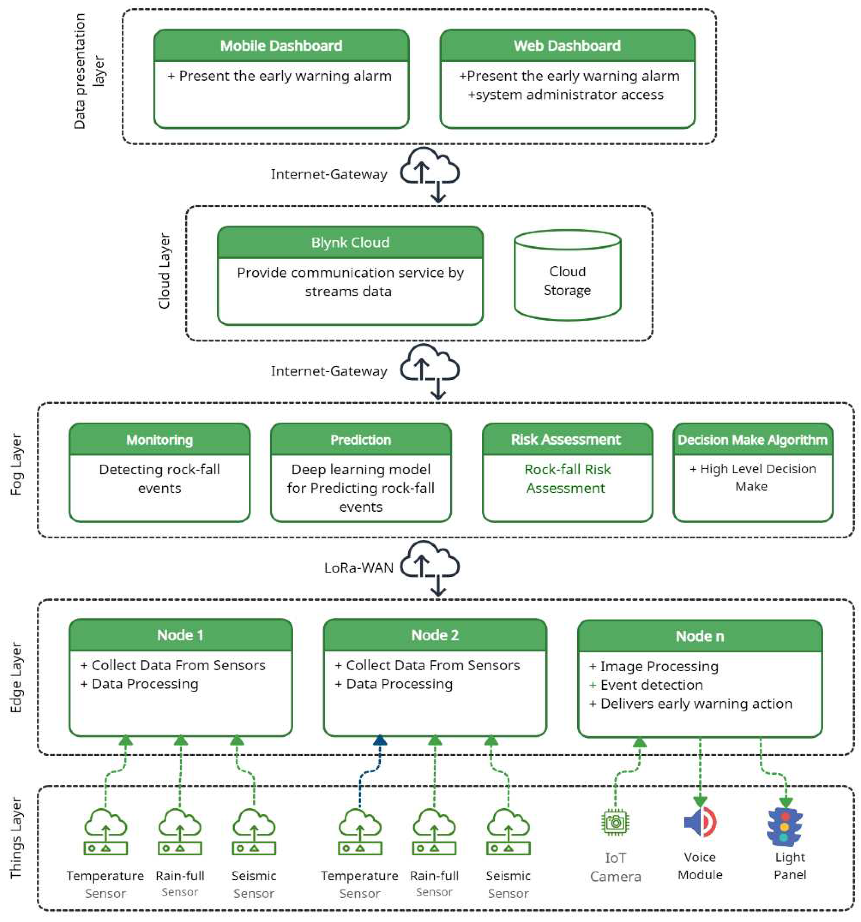
Figure 2.
Rock-fall detection model.
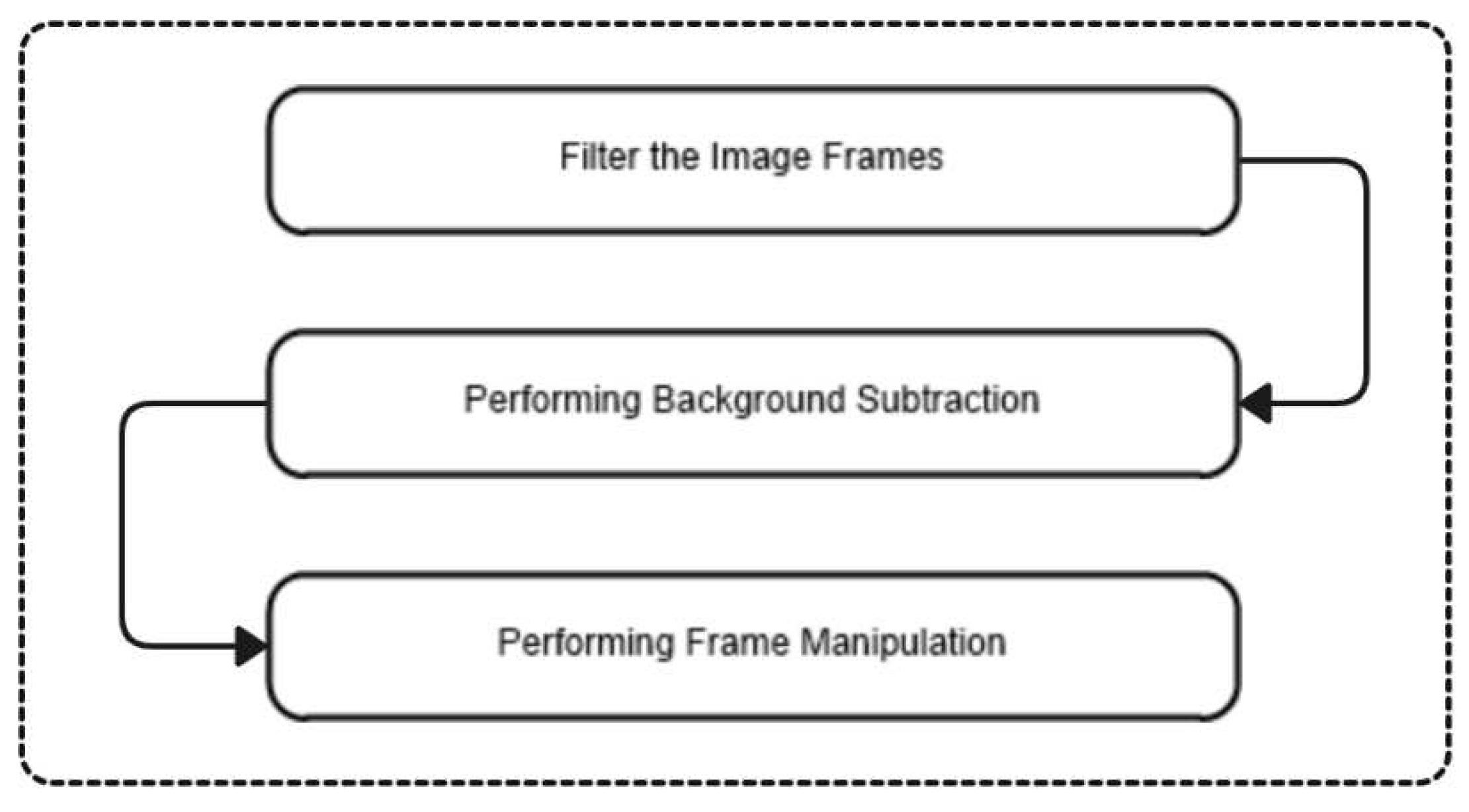
Figure 4.
The neuron’s main parts.
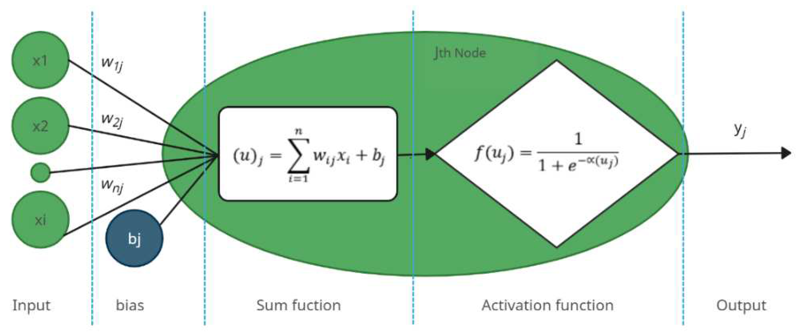
Figure 5.
Union of not mutually exclusive probabilities process.
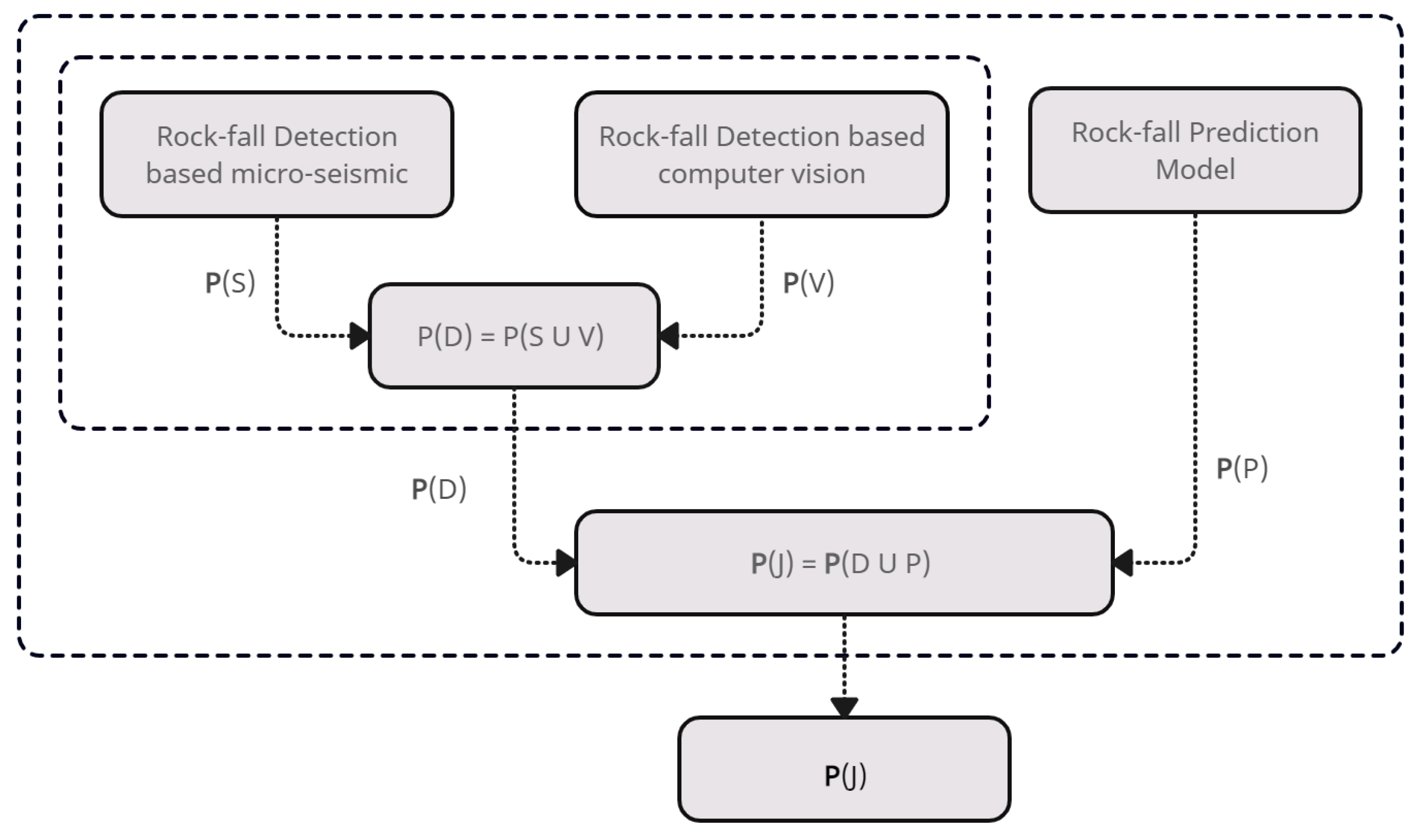
Figure 7.
The ROC curve (for validation data set).
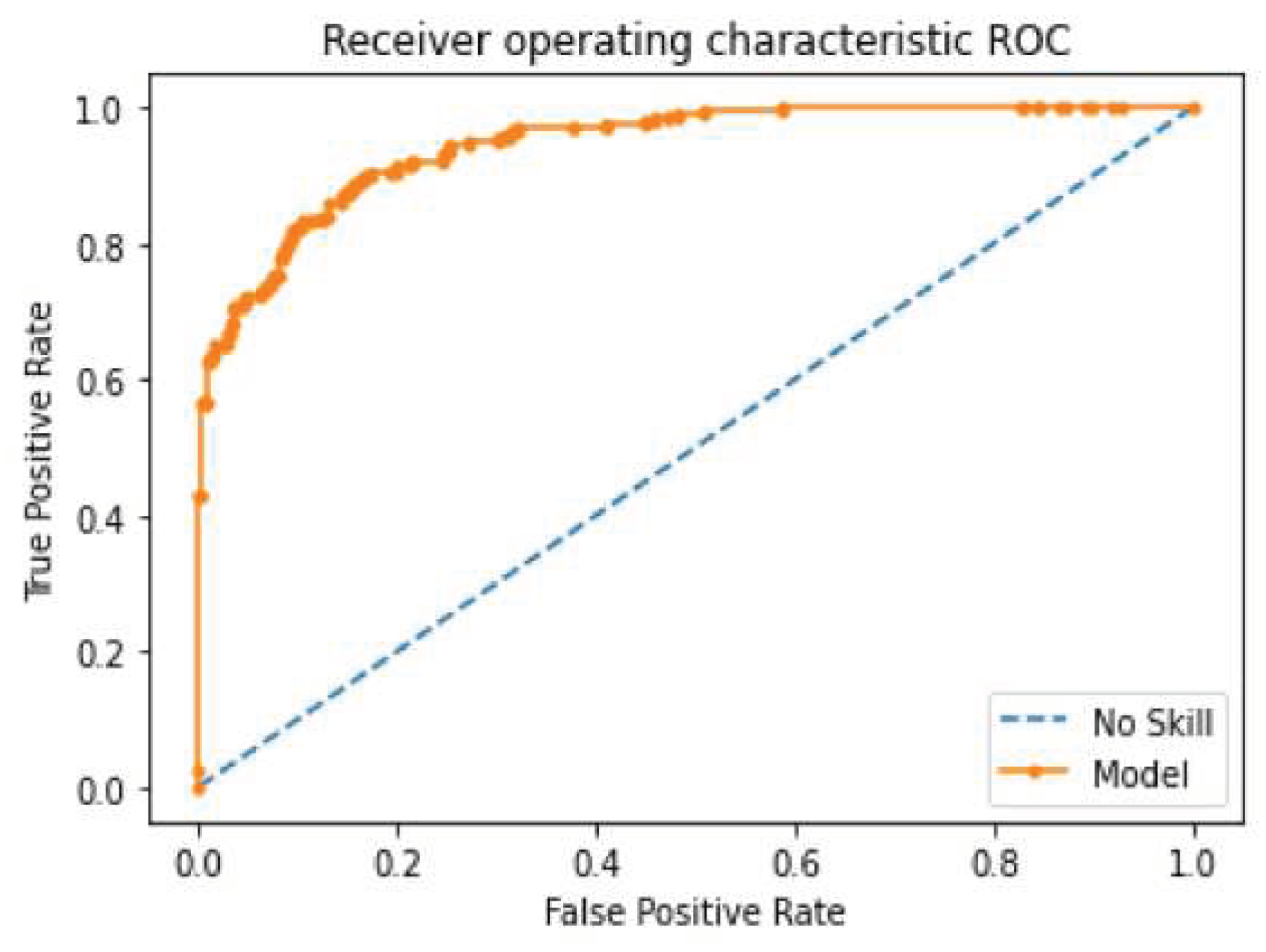
Figure 8.
The Rockfall Risk Probability.
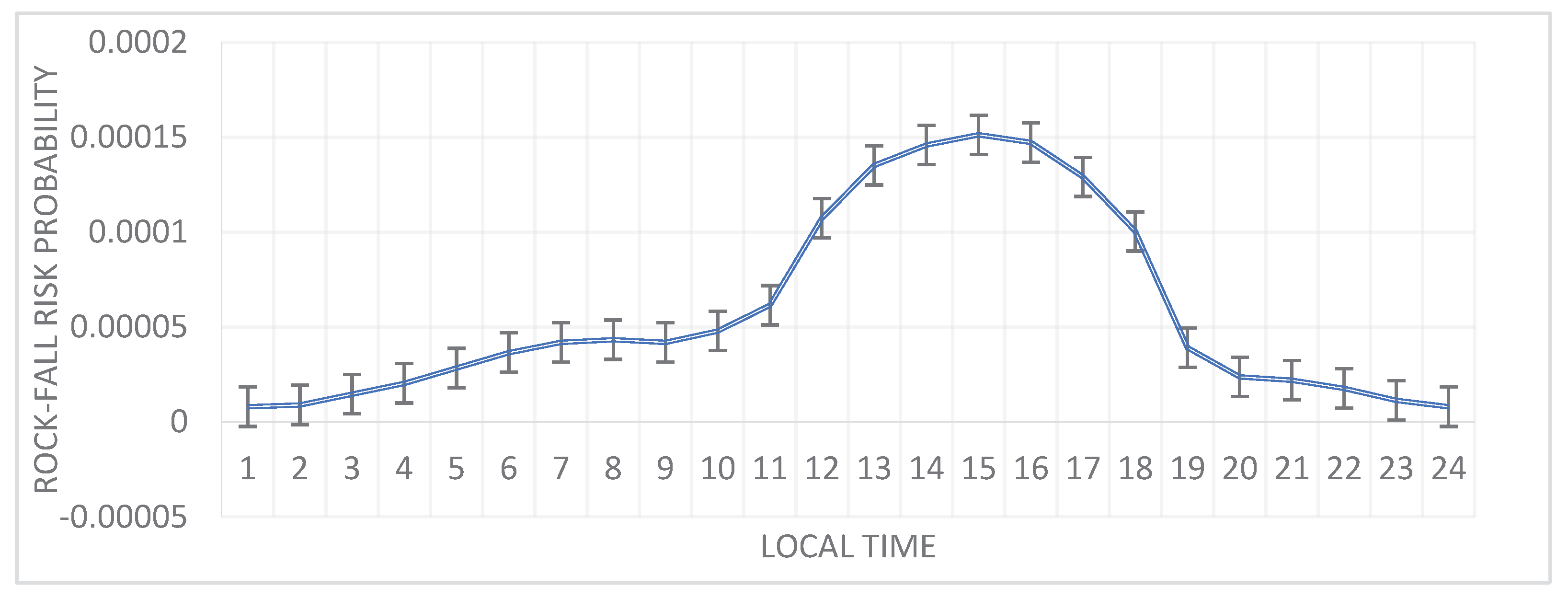
Figure 9.
ALARP thresholds triangle.
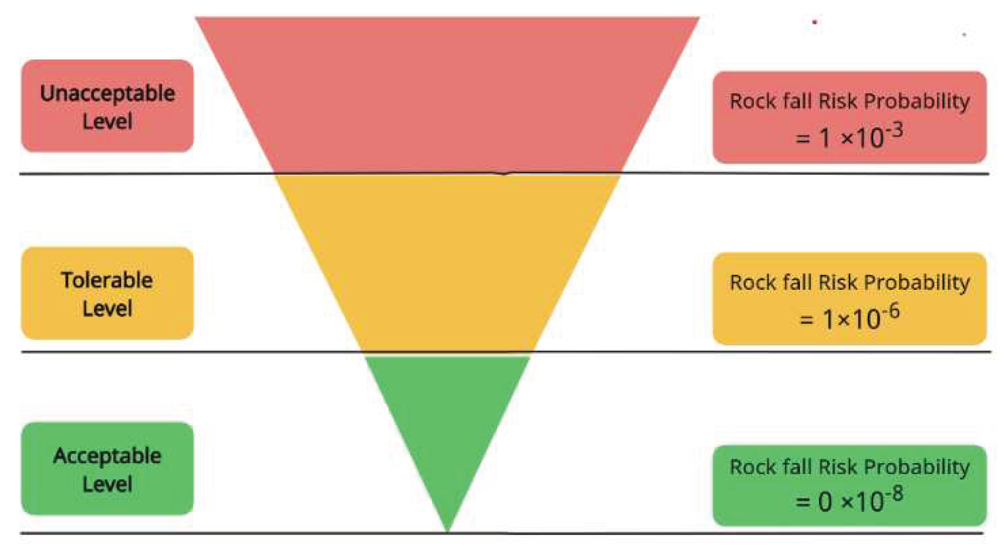
Figure 10.
The rock fall risk reduction.
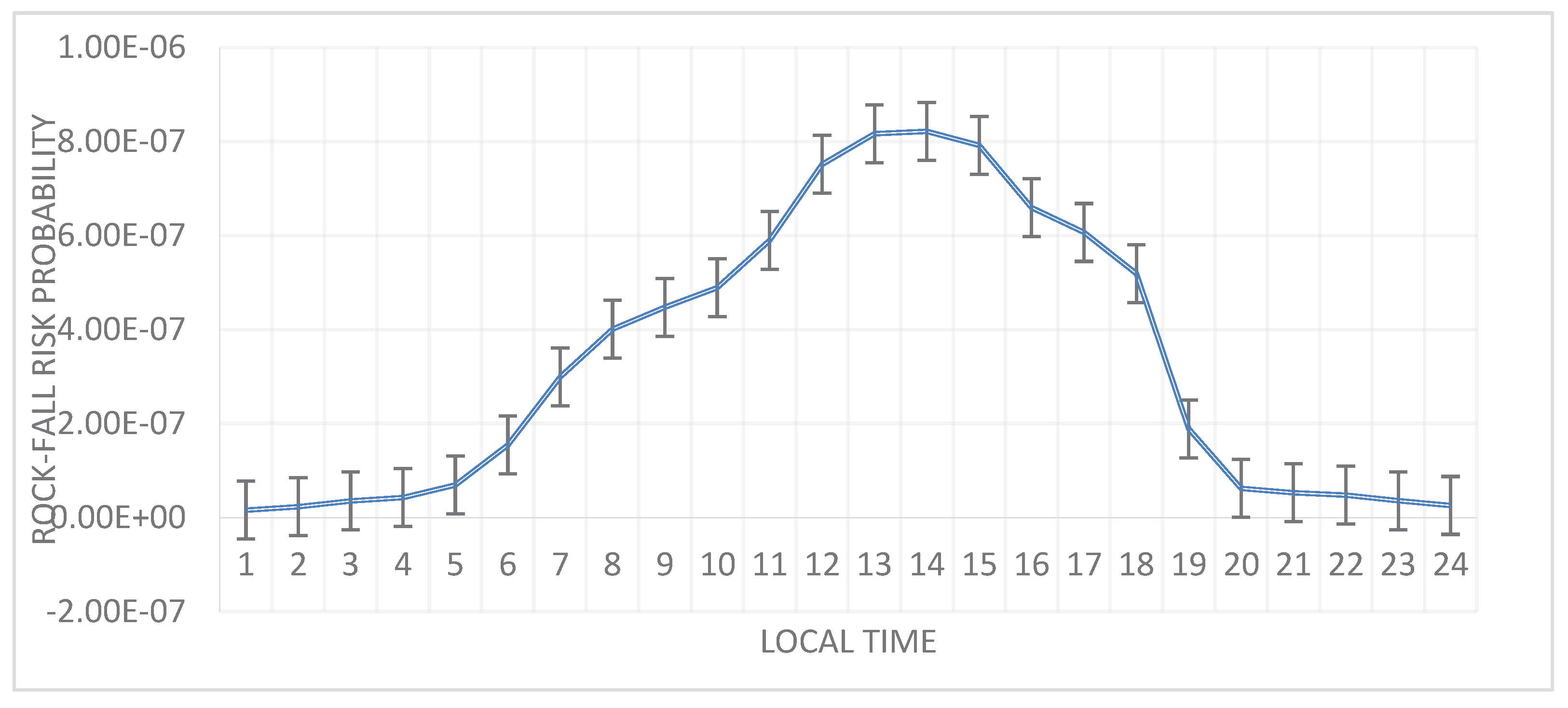
Table 2.
The average spectral amplitudes ratio R.
| frequency domain | frequency spectrum | R |
|---|---|---|
| first domain | 100Hz−1000Hz | 1.5±0.08 |
| second domain | 500Hz−1000Hz | 2.7±0.32 |
| third domain | 100Hz−500Hz | 7.1±0.68 |
Table 3.
The confusion matrix.
| Predicted (Even) | |||
|---|---|---|---|
| Not occurs 0 | Occurs 1 | ||
| Actual (Even) | Not occurs 0 | TN = 304 | FP = 51 |
| Occurs 1 | FN = 35 | TP = 222 | |
Table 4.
Clasification report.
| Class | Precision | Recall | F1-Score | Support |
|---|---|---|---|---|
| Rock-Fall Even (Not occur 0 ) | 91% | 86% | 88% | 355 |
| Rock-Fall Even (Occurs 1 ) | 81% | 86% | 84% | 275 |
| Accuracy | 86% | 612 | ||
| Macro avg | 85% | 86% | 86% | 612 |
Table 5.
Simulation setups.
| Parameter | Value |
|---|---|
| Average daily number of vehicles on the road (NV) | 8325 vehicles |
| Average vehicle lengths | 5.4 m |
| Brake Engagement time | 2 s |
| Driver reaction time | (0.4 to 2) s |
| Average acceleration | 10 m/s2 |
Table 7.
Model accuracy before and after augmentation.
| Rock fall Risk Prediction Model | Accuracy |
|---|---|
| Before Augmentation | 86% |
| After Augmentation | 98.8% |
Disclaimer/Publisher’s Note: The statements, opinions and data contained in all publications are solely those of the individual author(s) and contributor(s) and not of MDPI and/or the editor(s). MDPI and/or the editor(s) disclaim responsibility for any injury to people or property resulting from any ideas, methods, instructions or products referred to in the content. |
© 2024 by the authors. Licensee MDPI, Basel, Switzerland. This article is an open access article distributed under the terms and conditions of the Creative Commons Attribution (CC BY) license (https://creativecommons.org/licenses/by/4.0/).
Copyright: This open access article is published under a Creative Commons CC BY 4.0 license, which permit the free download, distribution, and reuse, provided that the author and preprint are cited in any reuse.


