1. Introduction
In the latter part of the 20
th century, optical computing became a subject of extensive research fueled in part by its inherent parallelism and the rapid development of laser technology. The new availability of bright coherent optical sources simplified phase coherent optical image processing. Simple lenses could be used to provide Fourier Transforms of optical images in parallel, at the speed of light (notwithstanding the fact that wired electrical signals also travel at the speed of light). Pattern recognition using real time holography became feasible and it was not long before content addressable memories and designs for neural networks began appearing. Electronic computational power continued to improve dramatically in terms of both processing speed and memory capacity. By the beginning of the 21
st century it was beginning to exceed the capabilities of optical systems. For example, optical compact disks and DVDs have now become practically obsolete, replaced by high-capacity solids state drives and cloud storage. There are, though, still applications where optics remains the best option. One example is data transmission over optical fibers. Particularly relevant here is the continuing interest in the design of neural networks using multimode fibers. As early as 1990, Aisawa et al. described image classification using multimode fibers followed by a multilevel network[
1]. Ancora et al. have shown that pattern classification can be accomplished using only a multimode fiber coupled with a single logistic regression layer[
2]
Propagation distances in optical fibers can result in the appearance of nonlinear effects. While these effects are often deleterious and require compensation, they can be used to good effect, for example in supercontinuum generation[
3]. Tegin et al. [
4] have shown that nonlinear effects in multimode fibers can be used to design optical neural networks whose power requirements can be lower than that of conventional electronic neural networks. Elements of a data set are represented optically using a spatial light modulator and transmitted through a multimode optical fiber. The authors showed that nonlinear interactions between the modes of the fiber can reformat the data into a “nearly linearly separable output data space” at the output of the fiber.
The original motivation behind the research presented in this paper was to explore the possibility of using another low power nonlinear optical effect, the photorefractive effect[
5], to perform similar transformations. This effect is a form of real time holography using optically induced refractive index variations in a medium to enable spatial mode mixing for use in optical transformations and computation. One possibility to use photorefractive mixing in a way that might be applied for model training is stimulated photorefractive scattering, known as fanning[
6]. The results presented here show that fanning can be well modelled with step sizes of the order of 2~5μm. The code can also be used to investigate other forms of photorefractive nonlinear coupling and generalized to other nonlinearities.
It was during the earlier period of intensive research into optical computing that most progress was made in the understanding and application of the photorefractive effect. A breakthrough took place with the discovery that ferroelectric crystals such as barium titanate, potassium niobate, and strontium barium niobate could support strong nonlinear optical interactions between low power, milliwatt level, continuous wave laser beams. This enabled the realization of many nonlinear optical devices that could otherwise only be achieved with high power pulsed lasers[
7] or with resonant materials such as sodium vapor[
8]. These included distortion compensating phase conjugate mirrors with reflectivity exceeding unity[
9], photorefractive oscillators[
10], and self-pumped phase conjugate mirrors[
10,
11].
In the early 90s we and others developed two-dimensional beam propagation codes to model photorefractive effects such as image amplification by two beam coupling and amplified photorefractive scattering[
6,
12,
13,
14,
15]. This amplified scattering is commonly known as fanning because of the characteristic fan shaped pattern observed in the far field. Over the past 30 years as computing power has improved it has become feasible to extend this model to three dimensions including time dependence. In this paper I describe the development of code implementing such a model (PRProp3D) for scalar fields. It is available as open-source software running in Google COLAB using its GPUs at
https://github.com/mcroning/PRProp3D. Limitations on the longitudinal step size are investigated in the context of tradeoffs between computation time and storage, and accuracy. The model has been checked against experimental data on image amplification, beam fanning, and time dependence. Sections in the paper treat
Image amplification with comparison to experimental data published by Fainman et al.[
16]
Beam fanning with comparison to prior theory by Zozulya et al[
13,
17] and new experiments.
Time dependence with comparison to high gain beam amplification experiments by Fischer et al[
18].
Theoretical appearance of high order diffraction at high gain described by Brown and Valley[
14]
The core of the program is a split step fast Fourier transform beam propagation method combined with a dimensionless model of the photorefractive effect. The Fourier method was chosen over finite difference methods because of its simplicity and comparable accuracy and computing time requirements. Propagation is divided into equal longitudinal steps of length
dz through the interaction region. Each computation step is divided into two parts. The first involves linear diffraction using the method of angular spectrum of plane waves[
19]. Linear absorption is neglected in the present realization but could be added easily. The photorefractive nonlinearity accumulated during the linear propagation step is then applied to the optical field as a thin transparency. Proper usage requires an understanding of the origin and management of several computational features, some of which are artifacts due to the periodic nature of the fast Fourier transform and the discrete step sizes involved in computational beam propagation. These artifacts are covered in detail in the appendix and include:
The appearance of excess high order diffraction over interaction lengths nominally in the Bragg regime. This effect decreases with decreasing longitudinal step size but does not tend to zero.
Coupling to the longitudinal grating formed by the equally spaced nonlinear transparencies. This feature is especially apparent in models of the fanning effect, in that it results in the appearance of rings centered on the direction of the incident beams in the far field where the fanning pattern is usually observed. The diameter of these rings is approximately proportional to the inverse of the square root of the step size. Step sizes less than 5mm will usually push the diameter of the innermost ring beyond the region of interest in the far field.
Wraparound effects due to the intrinsic periodic nature of the discrete Fourier transform. This last effect could be controlled by using finite difference beam propagation methods instead of FFT methods, but this would unnecessarily introduce additional complexity. We have chosen to continue to use FFT methods with the understanding that wraparound effects need to be acknowledged and minimized by choosing transverse apertures large enough to keep the main parts of the interacting beams away from the boundaries. We will see below that the periodic nature of the FFT is advantageous when seeking to verify the code against standard plane wave theory.
2. Methods
In keeping with the overall philosophy to try to keep the nonlinear propagation model as simple as possible while maintaining the principle physical behaviors we have chosen in the following to formulate the model using scalar diffraction. Extension to the full vector case including use of the dielectric tensor for beam propagation and electro-optic tensor for nonlinear grating formation would lead to a significant increase in complexity and we leave that generalization to future research.
The vector angular spectrum of plane waves method requires separate handling of the ordinary and extraordinary vector modes which are both dependent on the transverse spatial frequencies[
20].
Use of the full electro-optic tensor would require knowledge of the longitudinal components of the photorefractive space charge field which depend on the three-dimensional gradient of the optical intensity . The methods used in the past, and in this paper ignore the longitudinal component of the intensity gradient and space charge electric field: the grating is calculated assuming that it is independent of the optical fields at neighboring planes.
Nevertheless, the scalar quasi-3D method described below does match many experimental results.
2.1. Beam Propagation
The model describes the optical field in Cartesian coordinates with
x and
y transverse
z longitudinal. The input field is given in terms of its scalar amplitude
A(
x,y) at the input plane
z = 0. Propagation of the field amplitude
A(
x,y) by distance
dz is accomplished using the angular spectrum of plane waves method[
19]. The Fourier transform of the field is multiplied by the propagator
h for propagation over distance
dz:
where
f0 =
n/λ,
λ is the wavelength of the light,
n is refractive index, and
fx and
fy are the transverse spatial Fourier frequencies of the optical amplitude.
An inverse Fourier transformed is then performed to return the field to real space. The Fresnel approximation can be recovered by expanding the square root in the exponent to its first order Taylor expansion, but this leads to significant errors for the high angles of propagation that are commonly used. Discrete Fourier Transform wraparound effects are minimized by using a Tukey apodization window at each step.
2.2. Photorefractive Nonlinearity Model
The hopping model for the photorefractive effect, as originally published by Feinberg et al., was developed using the concept of charge carriers hopping between sites in a crystal with the hopping probability dependent on the local optical intensity and electric field[
21]. It can be rewritten in terms of continuous variables if it is assumed that only nearest neighbor hopping is important, that trapping sites can be treated as being uniformly spaced, and that there are many trapping sites in a single grating period so their distribution can be treated as a continuous variable. These approximations lead to a time dependent differential equation for the space charge electric field
E in terms of the spatially varying optical intensity
I which includes the equivalent dark intensity
Id to account for thermal relaxation. Primes represent spatial derivatives in the transverse direction. Full details may be found in
Appendix B.
3. Results
3.1. Two-Beam Coupling
As a check on the validity of the program we compared its output with predictions from the standard steady state coupled wave equations for two plane waves intersecting at half angle
θ in the slowly varying envelope approximation [
22]:
where
A1 is the electric field amplitude of the pump beam,
A2 is the amplitude of the signal beam and
γ p is the plane wave coupling constant:
where
n is the refractive index of the propagation medium,
kg the grating wavenumber normalized to the characteristic wavenumber
k0 and
E0 is the characteristic space charge field, both described in
Appendix B.
reff is the effective electrooptic coefficient[
23].
γ is the part of the coupling constant that is independent of propagation angles. The analytical solutions of these equations[
22,
24] show that the output beam ratio
rout in terms of the input beam ratio
rin is given by:
where the beam ratio is defined as the ratio of the intensity of beam 2 to that of beam 1.
Equivalently, the coupling constant length product (gain) can be written as
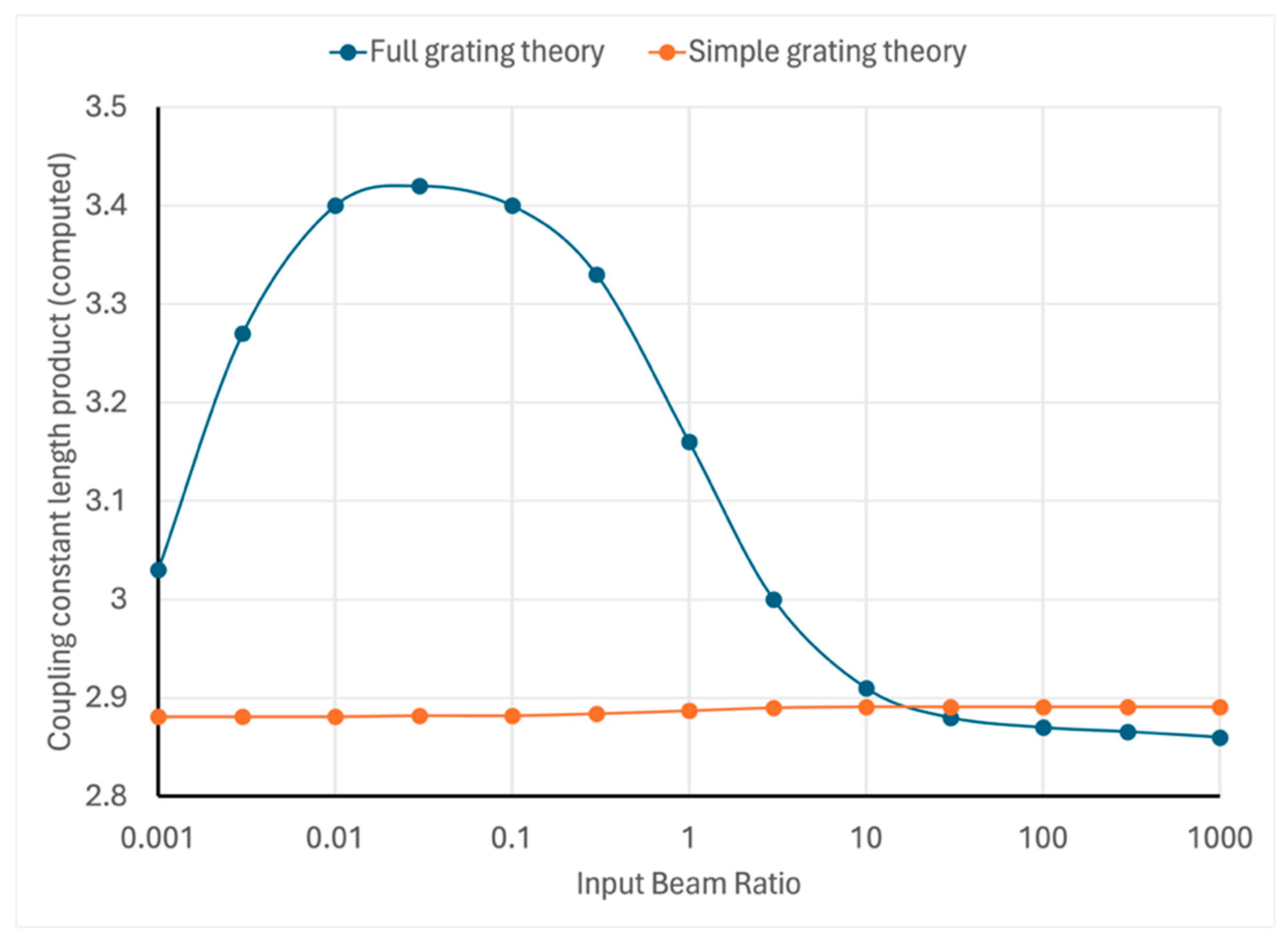
Figure 1 shows the gain calculated using equation (
7) from the output of the program when run with input gain
= 3 using both the generalized refractive index grating (equation(
3)) and the plane wave sinusoidal refractive index grating (equation (B11)). As can be expected, agreement with the plane wave coupled wave theory was better when using its specialized grating model. This infinite plane wave calculation is made possible in our code by taking advantage the fact that the periodic nature of the discrete Fourier transform implies that the beams have infinite transverse profiles. To prevent wraparound effects the beam crossing angles are chosen so that the grating is continuous across the boundaries and the peaks in Fourier space overlap from one Brillouin zone to the next. The Tukey window is not used. Allowable symmetric beam input angles are given by
where the integer
n is subject to
.
Δx is the transverse grid spacing and
Nx is the number of grid samples in the transverse
x direction.
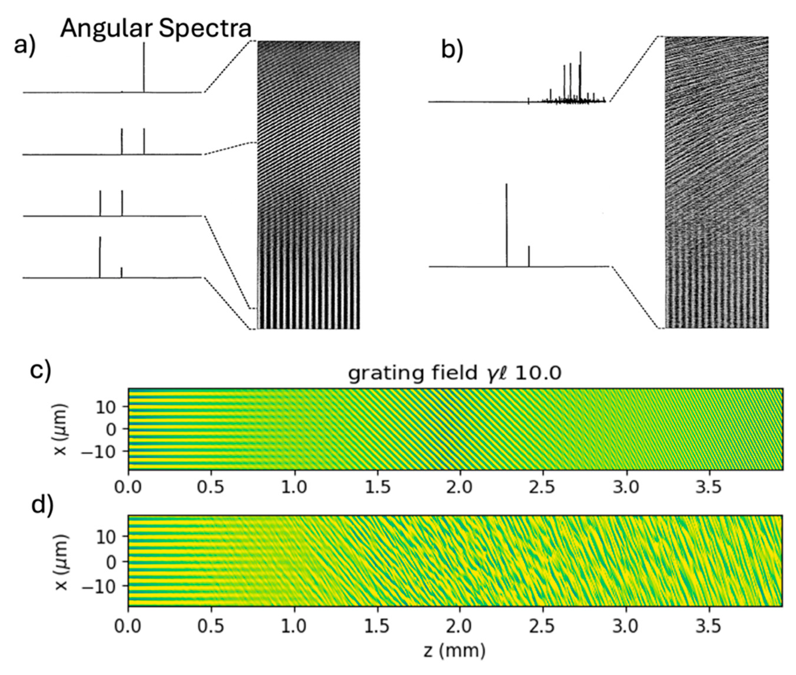
In 1993 Brown and Valley showed that two-dimensional beam propagation calculations for two-beam coupling at large coupling constants predicted the appearance and amplification of beams (kinky beams) diffracted by grating harmonics[
14]. The amplification of light scattered by these grating components would normally be considered forbidden by the Bragg condition and is not observed in practice. The authors hypothesized that the lack of experimental confirmation of these higher order beams is a result of their being overwhelmed by fanning. Our three-dimensional program reproduces these findings, as shown in
Figure 2.
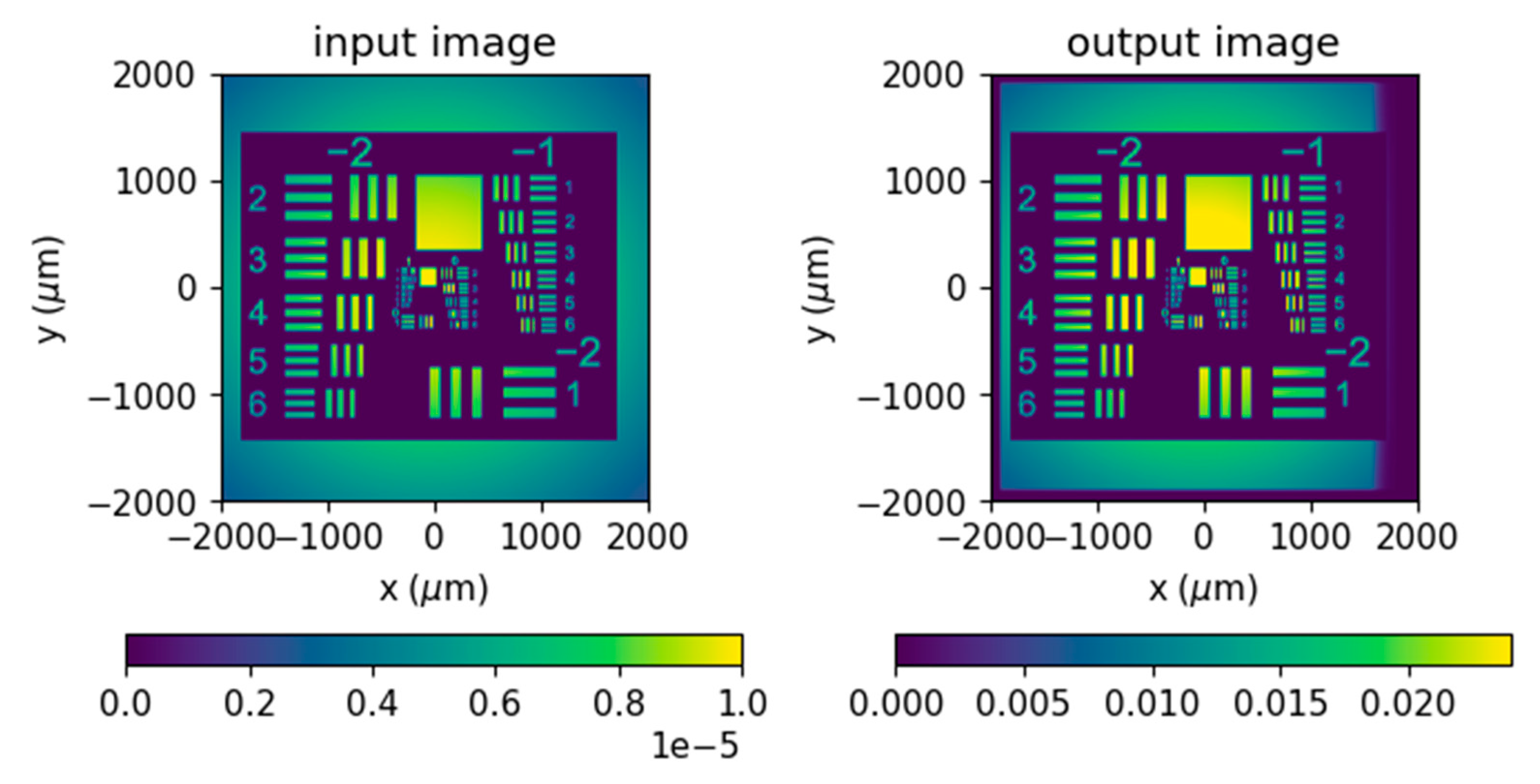
3.2. Image Amplification
One of the applications of photorefractive two beam coupling is coherent image amplification. Several authors have studied the fidelity of the process under various conditions. To see how well our code can model existing image amplification data, we modeled experiments in photorefractive barium titanate performed by Fainman et al. and treated by them using standard coupled wave theory[
16]. They presented their results in terms of absolute signal amplification
G0:
where
r =
rin is the ratio of the intensity of the signal beam to that of the pump beam.
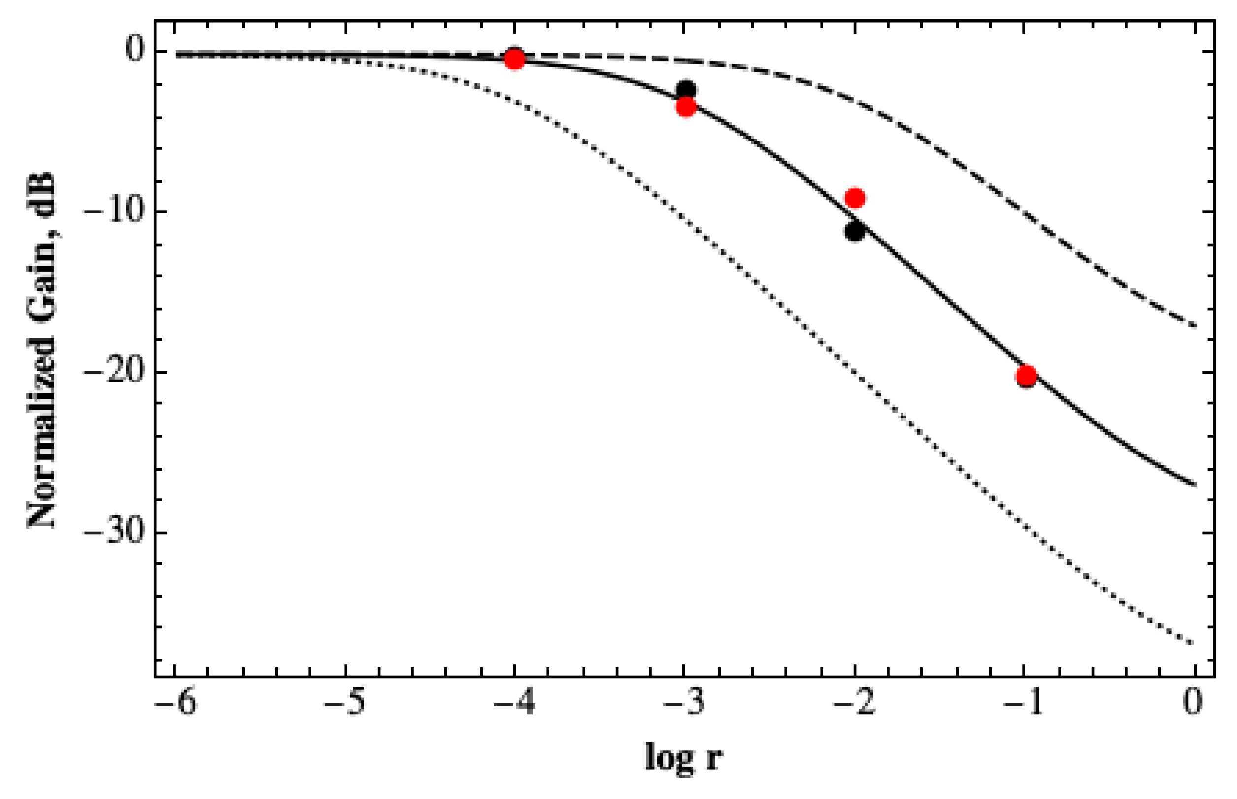
Figure 2 shows theoretical plots of normalized gain
where the saturated, small signal gain is
.
Figure 3.
Plots of normalized gain in dB versus input beam intensity ratio in the format used in reference [
16]. Coupled wave equation results are shown in the following lines: Dashed line; G
0sat=100, solid line; G
0sat=1000, dotted line; G
0sat=10,000. The black points are as calculated by the 3D program, and the red points are data from the experiment described in the reference. The results are so close that the data points sometimes overlap.
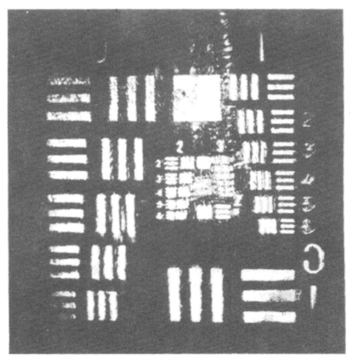
Reference[
16] treats image amplification optimization as its main result and we have reproduced some of the fidelity tests of that paper. While the group labels on the resolution targets are different, the computer input image has been scaled to the same size as the section of the chart shown in the amplified image from ref[
16].
Figure 4 and
Figure 5 show the comparisons for the small signal case treated in the Fainman paper. The dark stripe on the right of the output image in
Figure 4 is caused by the Tukey apodization at the grid edges.
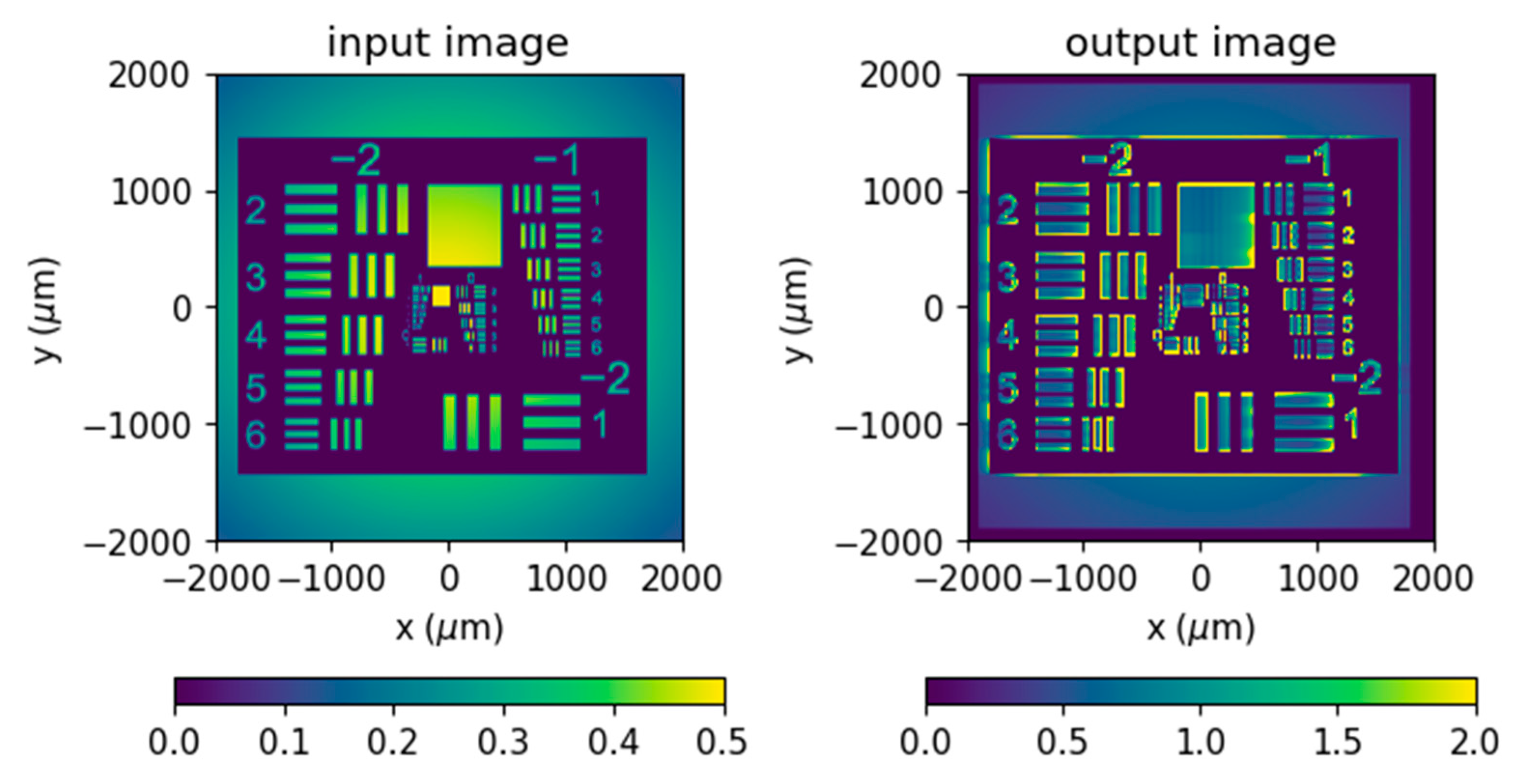
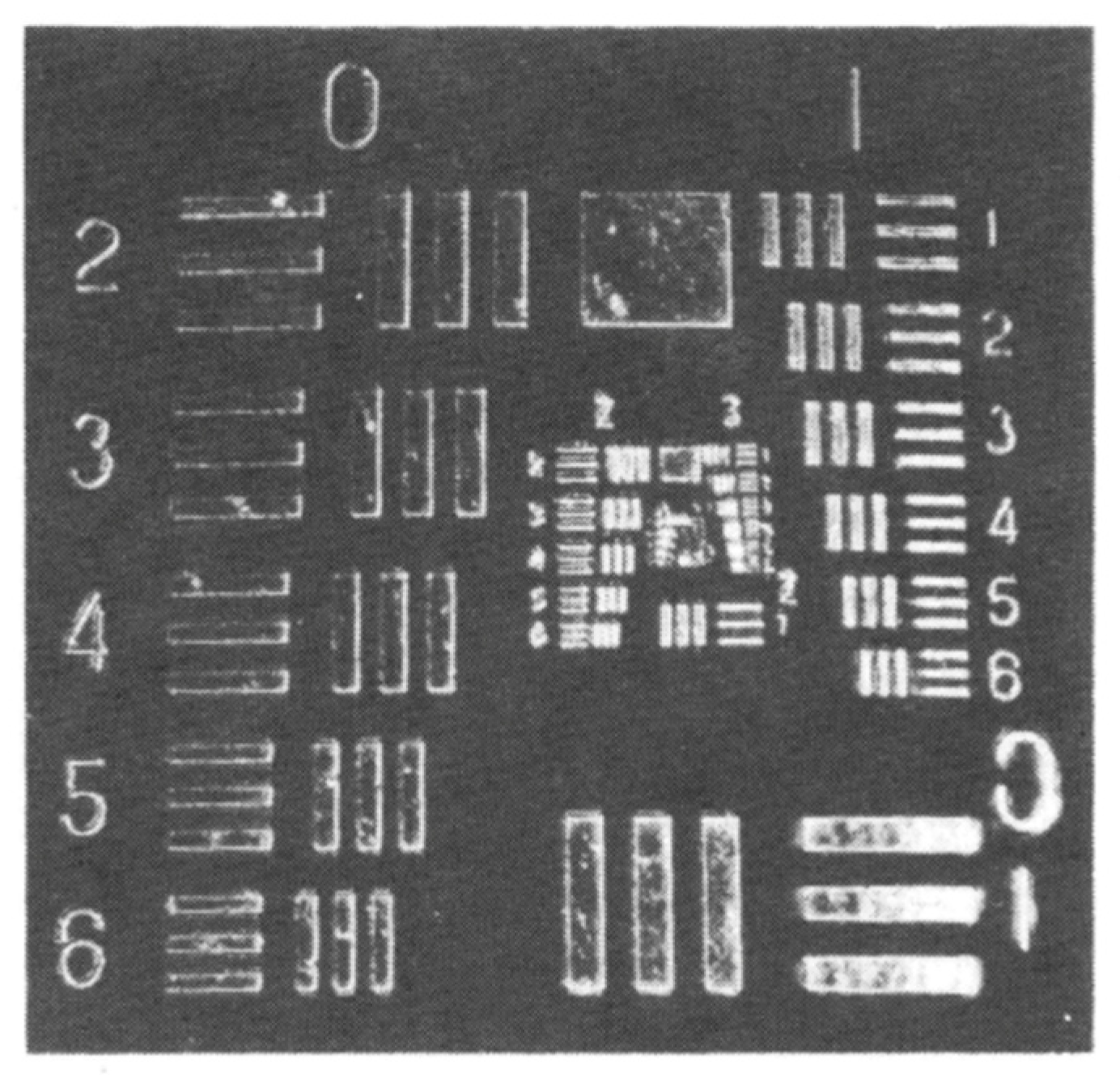
Reference[
16] shows that when the ratio of the input signal intensity to the pump intensity increases, the amplified image experiences edge enhancement because the high frequency parts of the image experience larger photorefractive gain than the low frequency components. This effect is reproduced by our model as shown in
Figure 6 and
Figure 7.
3.3. Photorefractive Amplified Scattering
The model allows for the three-dimensional simulation of photorefractive amplified scattering (fanning) seeded by optical scatterers[
25]. This fanning serves as the seed for various photorefractive oscillators such as unidirectional ring oscillators and self-pumped phase conjugate mirrors[
23] and contributes to noise in image amplification.
In 1994-5, Zozulya et al. published a two-dimensional computer model of the fanning effect and of several photorefractive phase conjugate mirrors[
13,
17]. This model used Crank-Nicholson integration of the coupled wave equations and a relaxation method for calculation of the photorefractive nonlinearity. We used their results as the basis for comparison for the output of our three-dimensional model. Following the method of Zozulya et al[
17] we modeled scattering noise in the crystal as a series of phase screens applied at each propagation step. The phase screens were represented as
where
ϕ is a two-dimensional array of normally distributed random numbers filtered spatially with a Gaussian kernel with standard deviation
σ. This standard deviation represents the scattering bandwidth in the transverse spatial spectrum. The corresponding angular scattering bandwidth is sin
-1(
σ/λ). The mean square deviation of
ϕ is given by
where
is a parameter representing the strength of the scattering and
Ns is the number of scattering screens.
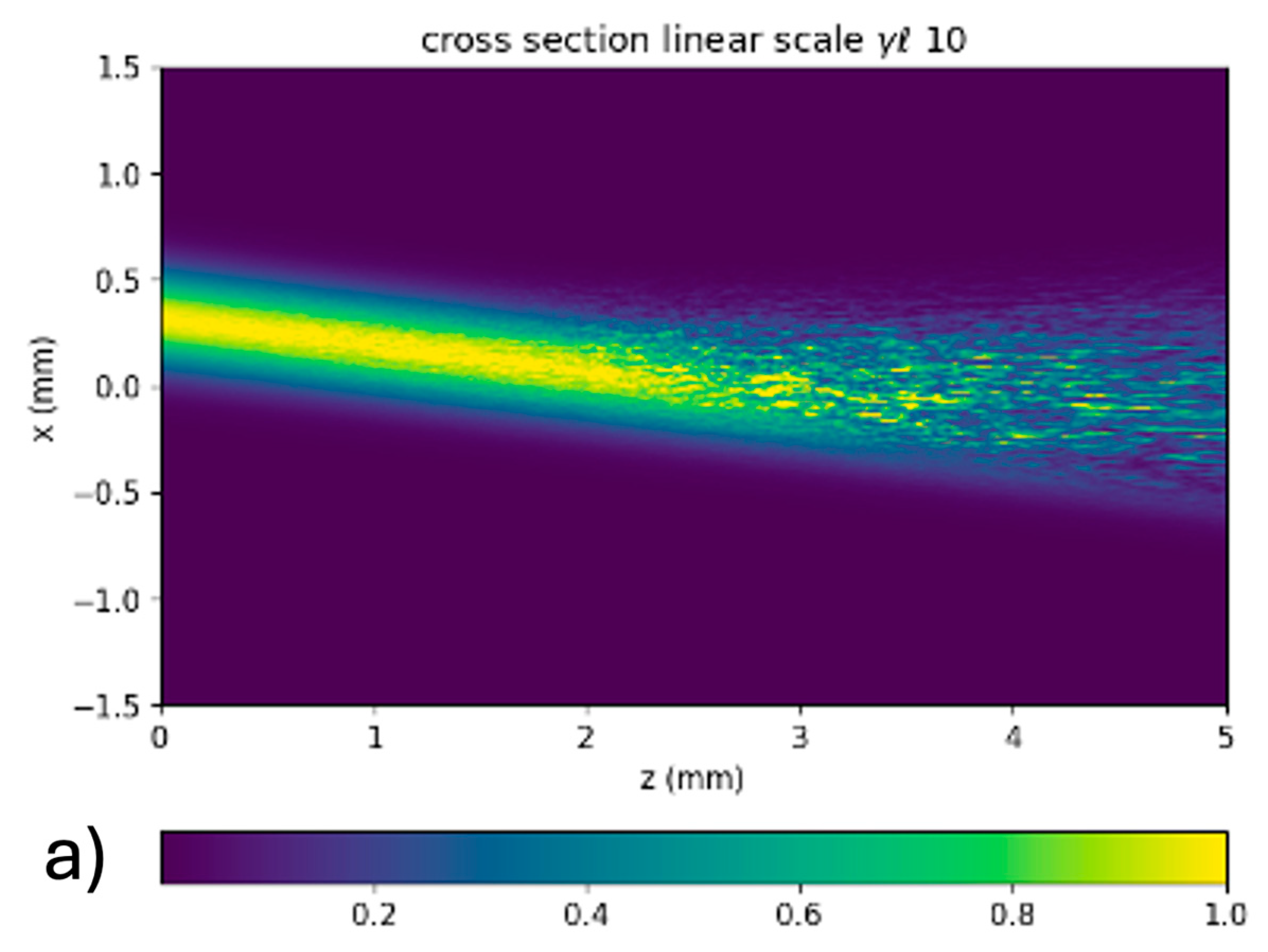
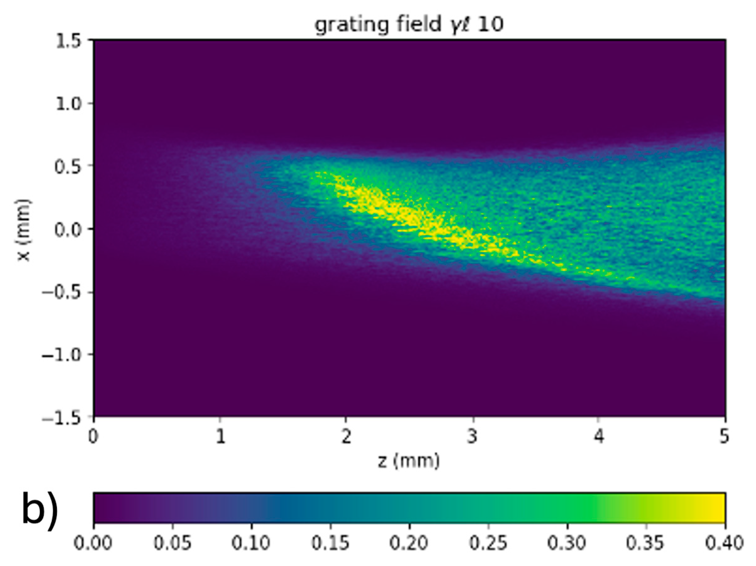
Figure 8 shows a fanning profile taken from Zozulya’s paper[
17] and
Figure 9 shows the corresponding results from our program. The relevant parameters are given in
Table 1
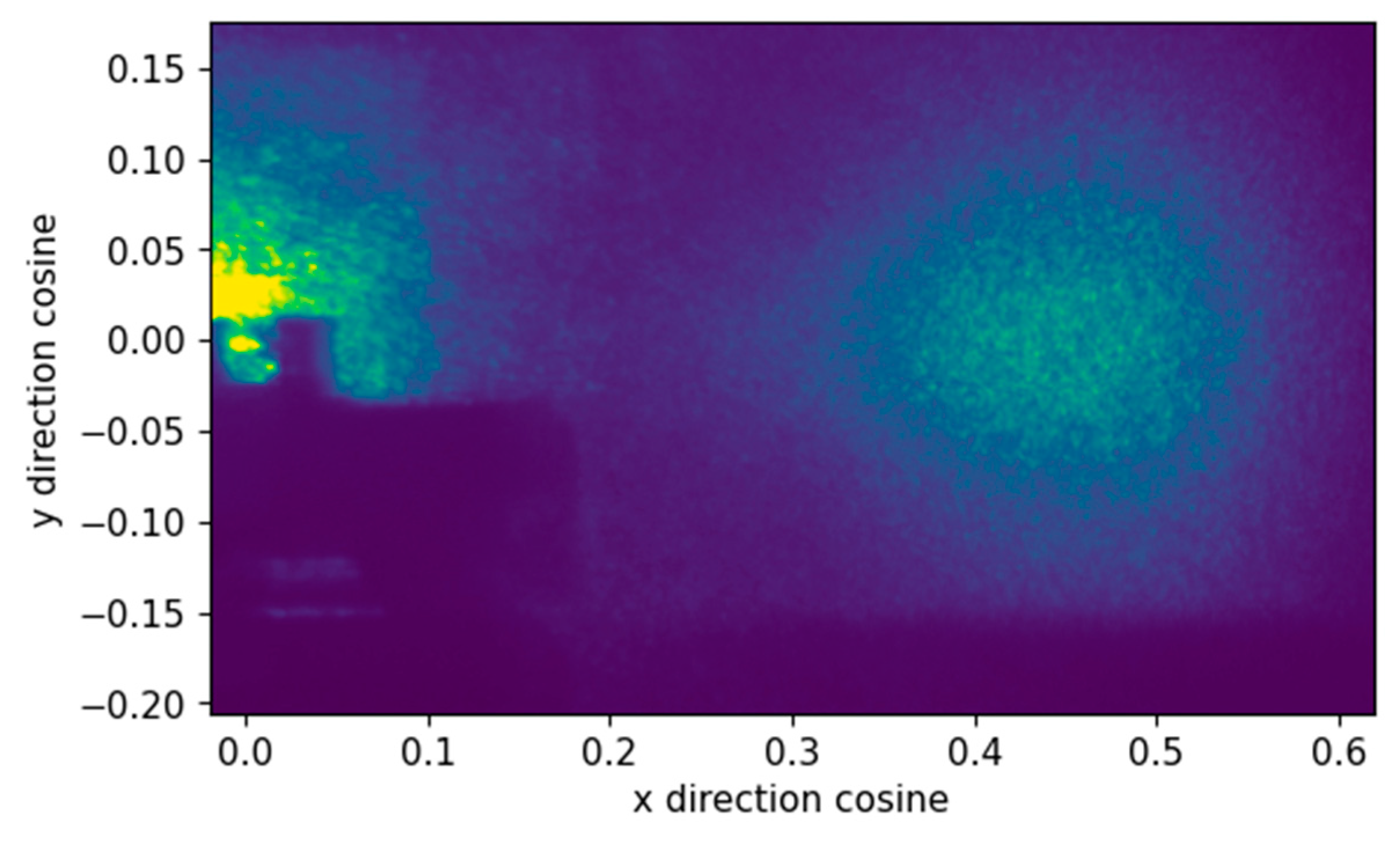
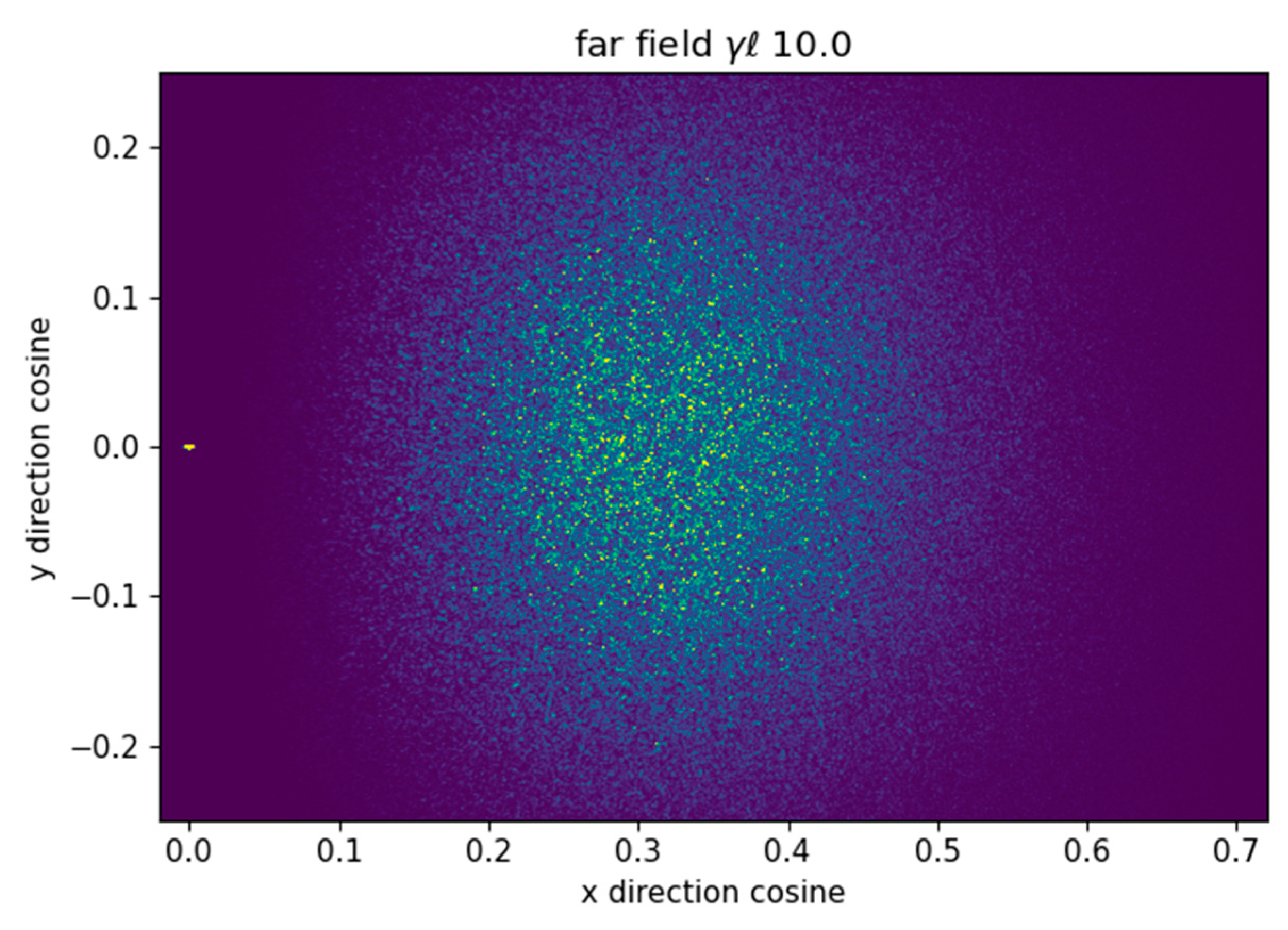
To provide a comparison of the transverse output of the code with experiment, we show in
Figure 10 an image of fanning of a 10mW 488nm beam from a Toptica iBeam smart diode laser after passage through a 6.5mm long crystal of barium titanate in our laboratory. The corresponding output of the model using beam waist 3mm and longitudinal step size 2μm and
=10 is shown in
Figure 11. The axes of these images are in terms of free space propagation direction cosines:
These are the components of the individual wavevectors in the beam along the x and y directions respectively. The direction cosines for propagation within the crystal may be found by dividing by the refractive index. In the paraxial approximation, these direction cosines can be interpreted as propagation angles in radians.
A disadvantage of using a scalar model rather than a vector model with the full electrooptic tensor is we do not reproduce the characteristic three lobed pattern of fanning in BaTiO
3 as modelled in the undepleted pump approximation by Montemezzani et al.[
26]. The development of these lobes can be seen in experiment video (
Movie S1) corresponding to the static image of
Figure 10. The central scattering angle calculated is less than that observed experimentally possibly because of a mismatch in the characteristic grating wavenumbers. Notice that in the video the underlying speckle pattern remains fixed as opposed to in observations characteristic of high intensities where thermal effects result in a time varying speckle pattern. `
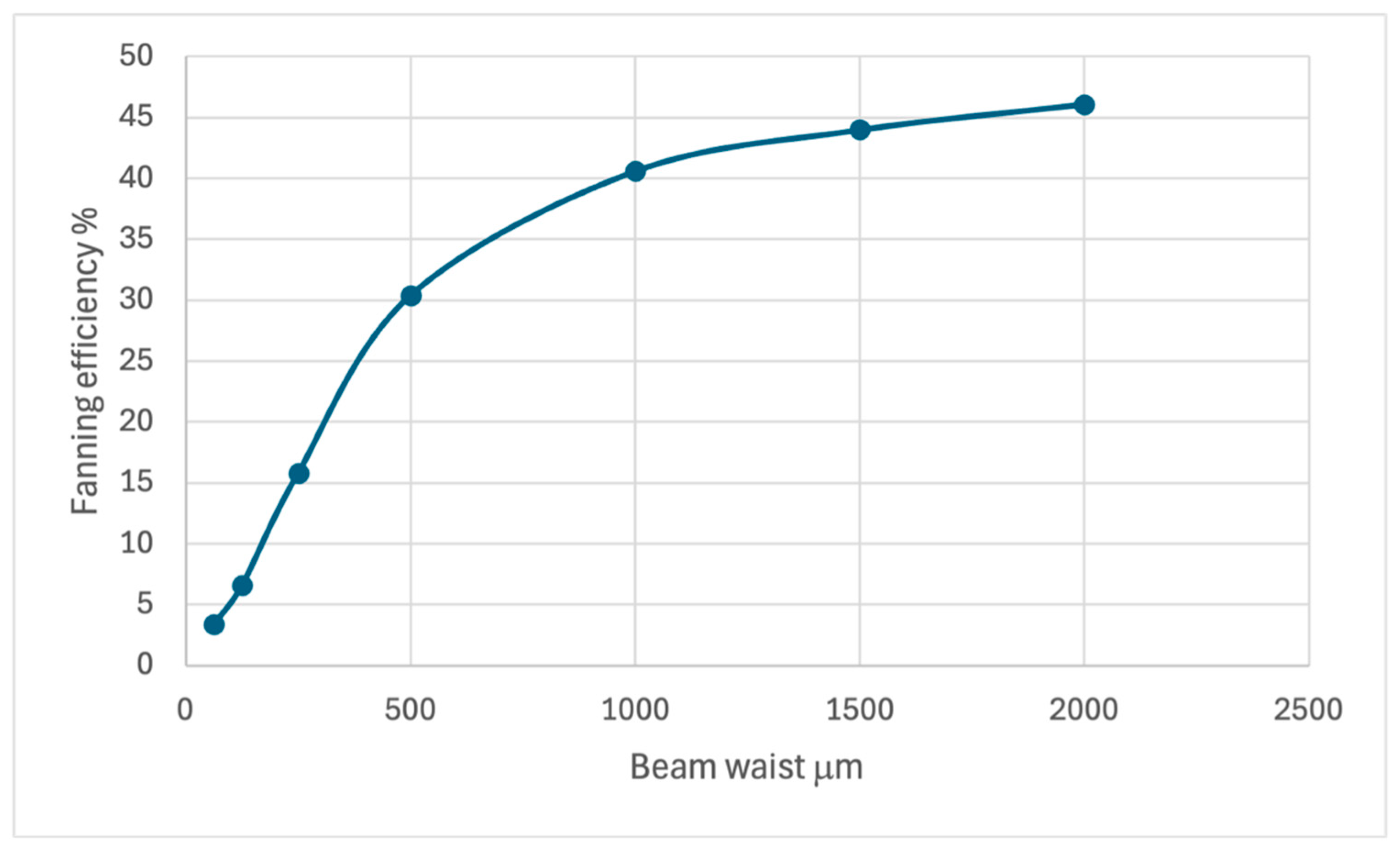
A question that arises about these fanning calculations is why large coupling constants of the order of
are required to reproduce experimental observations, while for modelling two beam coupling of gaussian beams or image amplification
suffices. One possible explanation is that the effective interaction length for fanning from narrow beams is limited.
Figure 12 shows how the calculated fanning efficiency increases with beam waist. Because of computer limitations, it is often necessary to perform fanning calculations for beam waists that are smaller than those encountered in the lab.
3.4. Time Dependence
The model includes the option to follow the time dependence of the buildup of the interactions by using numerical Euler integration of Equation Error! Reference source not found.
In all calculations that follow we use normalized time and normalized distance: see
Appendix B).
One of the main features of the photorefractive effect is that when the intensity of the interacting beams is above the dark intensity
Id, the steady state coupling strength is approximately independent of intensity. The tradeoff is that the response becomes slower as the intensity drops: when the intensity is larger than the equivalent dark intensity the response time is approximately inversely proportional to intensity. Additionally, when the coupling constant increases the gain response time also increases.
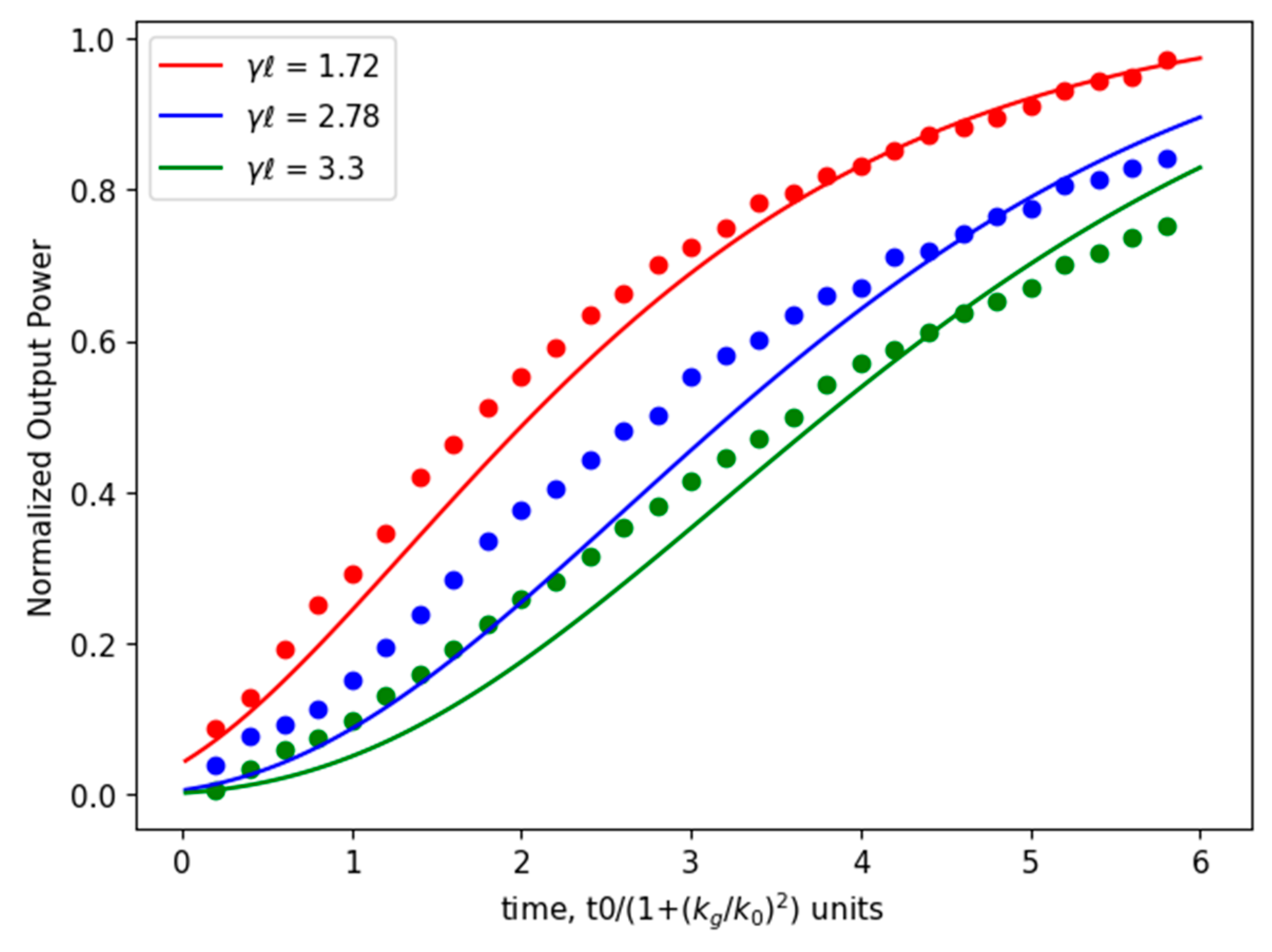
Figure 13 shows a comparison between the time behavior of two-beam coupling gain measured experimentally by Horowitz et al.[
18], and that predicted by the present software. These results match those from the basic time dependent model used in that paper. The dots represent the experimental data, and the solid lines represent our computed response. The response times are in accordance with the analytic estimate derived by Vachss[
27]:
3.5. Time Dependent Amplified Scattering
Here, we present a time dependent model of photorefractive fanning. the parameters are the same as for the static study of section 3.3 except the longitudinal step size had to be increased from 2μm to 8μm because of memory limitations. The calculation in the time dependent case requires the retention of the full three-dimensional grating distribution at the previous time step. This increased demand on memory can be mitigated by batching the grating distribution into the CPU.
The increased step size resulted in the appearance of ring artifacts whose origin is treated in
Appendix C below.
In the context of modelling the time dependence of fanning, we found that the integration could become unstable. We believe this is due to the high spatial frequencies in the fanning grating: the time constant decreases as the grating spatial frequency increases (see Equation (B11)). The stability criterion of Euler integration for simple exponential decay is |Δt/τ-1| < 1 [
28] so we can attempt to ensure stability of the integration by making the size of the time steps substantially less than the shortest time constant
tmin of the system. The grating wavenumber cannot be larger than 2π times the maximum frequency of the model in Fourier space so using Equation (B11) we choose the step size conservatively to be
where
Nx is the number of samples in the transverse direction and
L is the transverse aperture of the crystal.
Because we have made this empirical choice for time steps and because we are solving a space-time partial differential equation, not an ordinary differential equation as is usually the case for Euler integration, it is important to provide a monitor for instability in the program’s calculation. Such an instability manifests itself in the generation of exponentially growing values in the grating space charge field. We abort the calculation loop upon the occurrence of a NaN in the space charge field. For our purposes the method used for setting time step sizes has been found to be sufficient. The development of adaptive step sizes and better convergence criteria and integration methods could be addressed in future research.
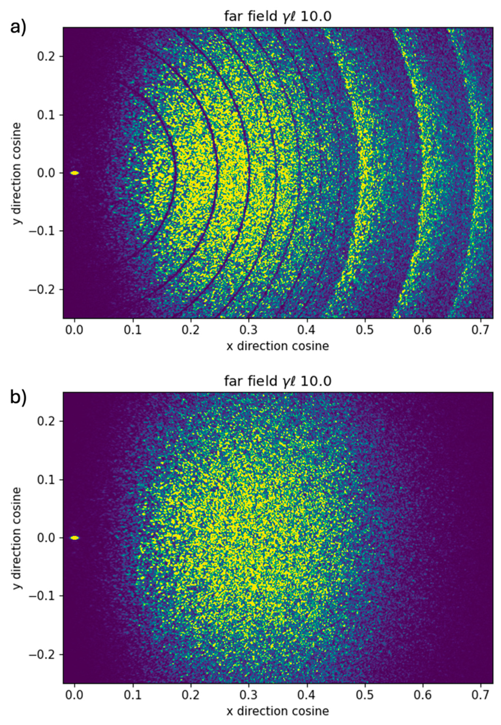
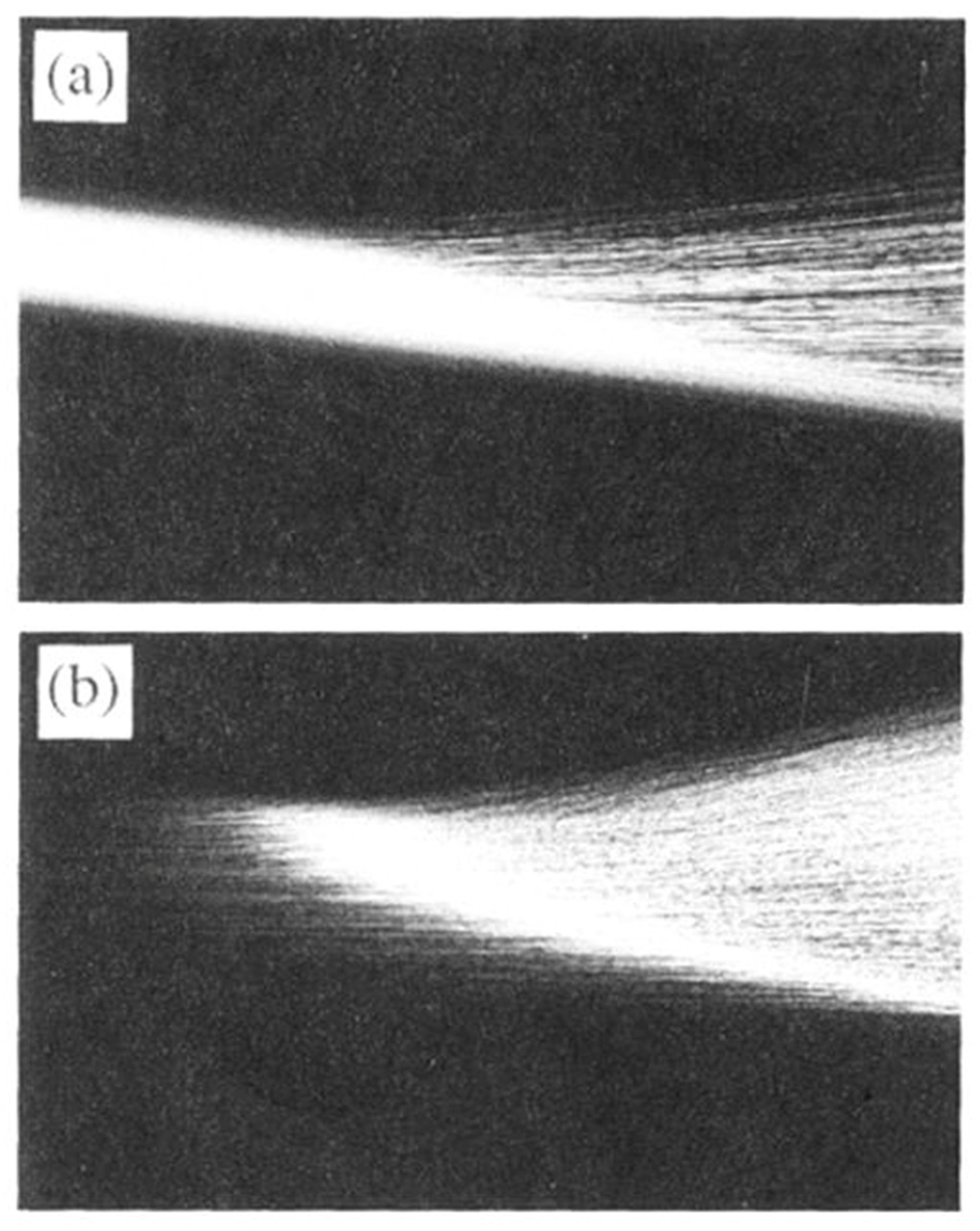
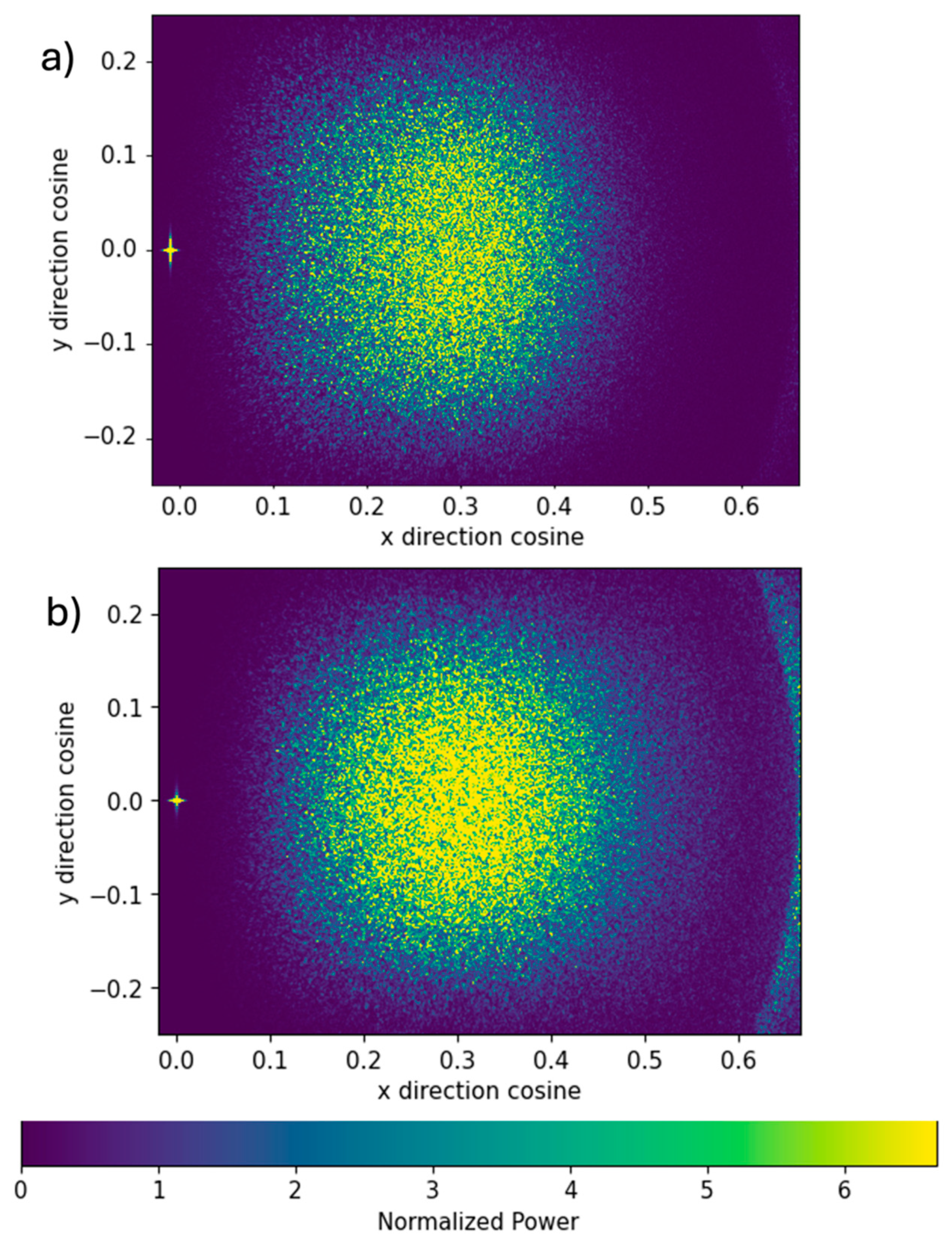
Figure 14 shows (a) the fanning far field computed by the time dependent algorithm at the end of 10 characteristic time constants
t0 and (b) by the static algorithm. The experiment and time dependent calculation videos can be found in the
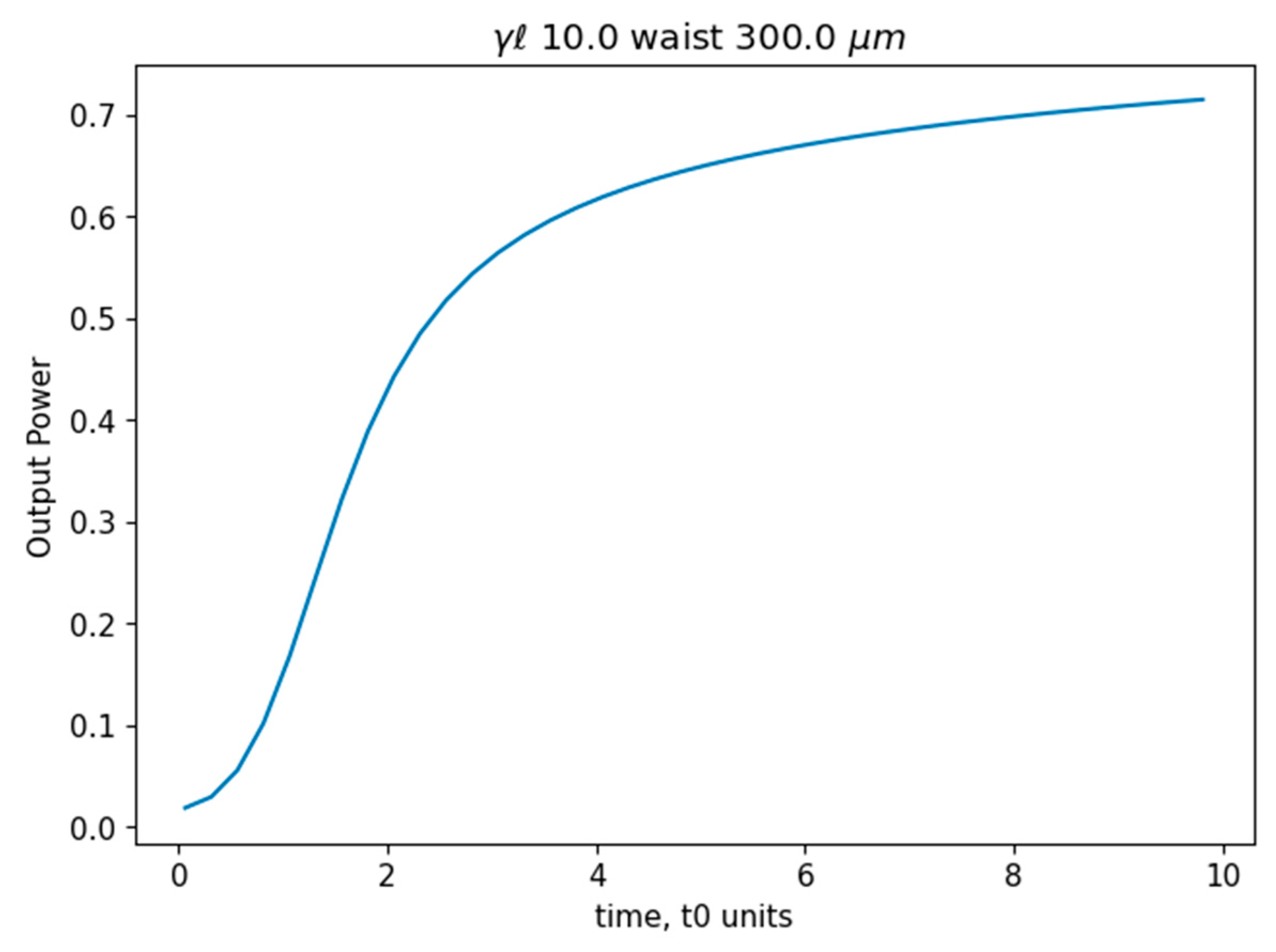
supplemental materials (Move S1 and S2). The far field generated by the time dependent model is not quite fully developed, as is evidenced by the more pronounced appearance of the additional artifact in the static model output. The artifacts can be a significant calculational sink of true fanning power and efficiency. The time dependence of the fanning power, shown in
Figure 15 is consistent with the coupling constant related lengthening of two beam coupling response times described above.
4. Discussion
The split step beam propagation model has already been successfully applied to many photorefractive phenomena starting in the early 1990’s. These include image amplification, photorefractive oscillators, self-pumped phase conjugate mirrors, photorefractive surface waves and optical solitons. To the best of my knowledge, however, there had been at least four gaps in knowledge about the method:
Validity of the method and its computational limitations. Many of the prior results concentrated on analyzing the fields within the crystal, not the far field output. It is in the far field that deficiencies of the model are most apparent through the appearance of scattering ring computational artifacts. In this paper we have given some guidelines for the mitigation of these artifacts, mainly by the judicious choice of propagation step sizes.
Extension of the scalar model from two to three dimensions. This has been enabled by improvements in available computational power since the 1990’s, in terms of data storage, random access memory, the availability of multicore processors and GPUs for parallel processing.
Extension of the model from scalar to vector fields and the ability to model propagation in birefringent crystals considering the full electrooptic tensor.
Inclusion of thermal effects. These become important when the intensity of the beams becomes so large that temperature dependent refractive index changes important. This effect can be significant since many photorefractive crystals are ferroelectric crystals near their Curie temperatures.
This paper has addressed the first two of these gaps and has given guidelines for proper usage. We found that propagation steps shorter than a few (~4) wavelengths are usually sufficient to push the artifacts’ direction cosines out of propagation range, that is greater than unity. On the other hand, longer steps can be used to reduce computation time for the interaction of beams with slow transverse variation. An example is two beam coupling of 100μm waist gaussian beams.
The original application that originally motivated this study: the use of photorefractive fanning mode mixing for deep learning was not successful. While a photorefractive fanning layer followed by a single fully connected layer could indeed be used to classify audio and regular MNIST data sets, the results were no better than those previously obtained using linear mode mixing in multimode fibers[
1,
2]. I hope, however, that the extension of the scalar model to three-dimensions, discussion of its capabilities and limitations, and the associated open-source Python software will be of use to researchers in the future.
5. Conclusions
This paper is an elaboration of a paper published by my group at Tufts University of a “whole beam” method for photorefractive nonlinear optical beam propagation[
12]. That paper was motivated by a need for a photorefractive theory that went beyond the standard slowly varying envelope coupled wave theory to address spatial effects on image bearing and multiwavelength beams and was subsequently used in a two dimensional study of fanning in my group [
29]. We have presented here a realization of the scalar split step method in three dimensions and have used it to revisit several prior results on fanning, image amplification, high gain effects, and the time dependence of the processes.
Supplementary Materials
The following supporting information can be downloaded at the website of this paper posted on Preprints.org, Movie S1: Experimentally observed growth of fanning, Movie S2: Calculated growth of fanning, JSON files containing the parameters used for figure calculations.
Funding
This research received no external funding.
Data Availability Statement
Conflicts of Interest
The authors declare no conflicts of interest.
Appendix A. Program Description
The program calculates unidirectional nonlinear optical beam propagation in three dimensions using photorefractive optical nonlinearities. It is based on the well-known split step beam propagation method which divides the process into a series of alternating steps along the longitudinal
z direction. Diffractive propagation steps are handled using the angular spectrum of plane waves method[
19] in which the angular spectrum of the optical field is calculated using the Fast Fourier Transform (FFT). The field is propagated as a set of individual plane waves for a short distance
dz after which the inverse Fourier transform is taken to return to real space. The accumulated nonlinearity is then calculated from the intensity and applied as a spatially varying transparency. The process is repeated until the end of the interaction region is reached.
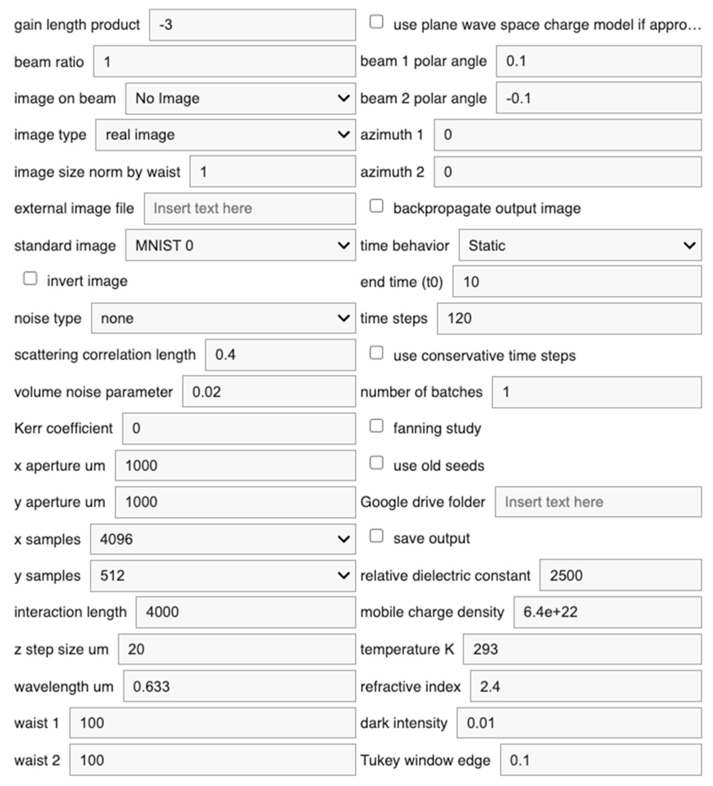
The parameters used in the code are as follows, listed in the order that they appear in the input form. They are stored for use in the program a dictionary named ‘prdata’. This dictionary may be saved to facilitate reproduction of results at a later time
Figure A1.
Typical PRProp3D program input form.
Figure A1.
Typical PRProp3D program input form.
gain length product: The standard interaction strength used in the plane wave photorefractive theory. It is the length of the interaction region times the coupling constant γ corresponding to the case where the grating wavenumber kg equals the characteristic wavenumber k0.
beam ratio: The ratio of the peak intensity of beam 2 to beam 1. This corresponds to the parameter r in the plane wave theory. While this paper is written in terms of beam 2 being the signal and beam 1 the pump, it is beam 1 which is most closely monitored in the program. Amplification of beam 1 requires that the gain be set negative.
image on beam: A dropdown to specify whether an image is to be applied at the input to one or both beams. This is useful for examining the nonlinearity induced image distortions.
image type: Determines whether the image is applied as an amplitude or phase transparency.
image size normalized by waist: The ratio between the transverse extent of the image to the waist of beam 1.
external image file: The path in a Google drive to a user supplied image for application the input. If there is no file at the path specified, the image specified in the standard image dropdown will be used if called for.
standard image: This dropdown is used to specify which of eleven standard supplied images will be used. One example of an MNIST digit for each of the digits 0 through 9 is supplied, as well as a 1951 Air Force Resolution Chart.
invert image: A toggle to provide the option to invert the gray scale of the input image. This is sometimes useful for avoiding sharp edges at the image boundary.
noise type:
none: No noise
volume xy: Scattering screens are placed at the end of each propagation step with the nonlinear phase transparency. The correlation length of these screens is given by sigma (see parameter sigma below). They are uncorrelated in the z direction.
scattering correlation length: The correlation length (μm) of the Gaussian random phase screens used to model optical scattering in the crystal.
volume noise parameter: scattering amplitude parameter ε: Number of scattering phase screens times mean square deviation of each phase screen.
Kerr coefficient: magnitude of any nonlinearity that is directly proportional to the local intensity such as those due to thermal effects.
x aperture um: The transverse extent in micrometers of the interaction region in the x direction.
y aperture um: The transverse extent in micrometers of the interaction region in the y direction.
x samples: Number of grid points in the x direction.
y samples: Number of grid points in the y direction.
interaction length: Length in micrometers of interaction region in z direction. Normally, the propagation axes of the two beams, beam 1 and beam 2 will be in the xz plane (azimuth zero, see below).
z step um: The longitudinal step size in micrometers. Proper modelling of the optical effects of fine (micrometer scale) refractive index variations often requires step sizes of 10μm or less.
wavelength um: Optical wavelength in free space in micrometers.
waist 1: The input beams are generated using the standard gaussian beam formula. The waist of beam 1 at its focus is waist 1. Its focus is halfway along the interaction length. If the beam waist is entered as a negative number, plane wave incidence is assumed, This can be used for cross checking results with the standard plane wave two beam coupling theory[
24]. If checked, the beam incidence angles will be set symmetrically to the wraparound effect free angles closest to the one initially specified in the beam 1 polar angle field. See Equation (8).
waist 2: The waist of beam 2.
use plane wave space charge model if appropriate: For use when using plane wave two beam coupling theory. Only available for two coupled plane waves propagating in xz plane with symmetric incidence angles.
beam 1 polar angle: The polar angle of incidence of beam 1,
. The definition of the angles is shown in
Figure A3.
beam 2 polar angle: The polar angle of incidence of beam 2,
azimuth 1: The azimuth of beam 1,
azimuth 2: The azimuth of beam 1,
backpropagate output image: This gives the option to backpropagate the output field in beam 1 to the input plane without nonlinearities to allow comparison of images before and after photorefractive image processing, for example amplification. Without backpropagation, regular diffractive effects appear which can obscure distortions due to the photorefractive effect. Backpropagation is equivalent to bringing the output to an image plane.
time behavior: Choosing “Static” invokes the time independent model where the partial derivatives with respect to time are set to zero. Choosing “Time Dependent” invokes the full time dependent model and generates movies showing time dependence and a graph of the power in beam 1 as a function of time as it is amplified or deamplified via two beam coupling. Time dependent calculations place a significant load on memory, since the full three-dimensional space charge electric field must be stored from one time step to the next.
end-time: The duration of the simulation in units of the characteristic time t0 (see appendix B). One time step equals the end-time/number of time steps.
time steps: the number of time steps taken by the model before completion.
use conservative time steps: Set the time step to one fourth of the minimum anticipated time constant, 1/(1+(kg/k0)2)
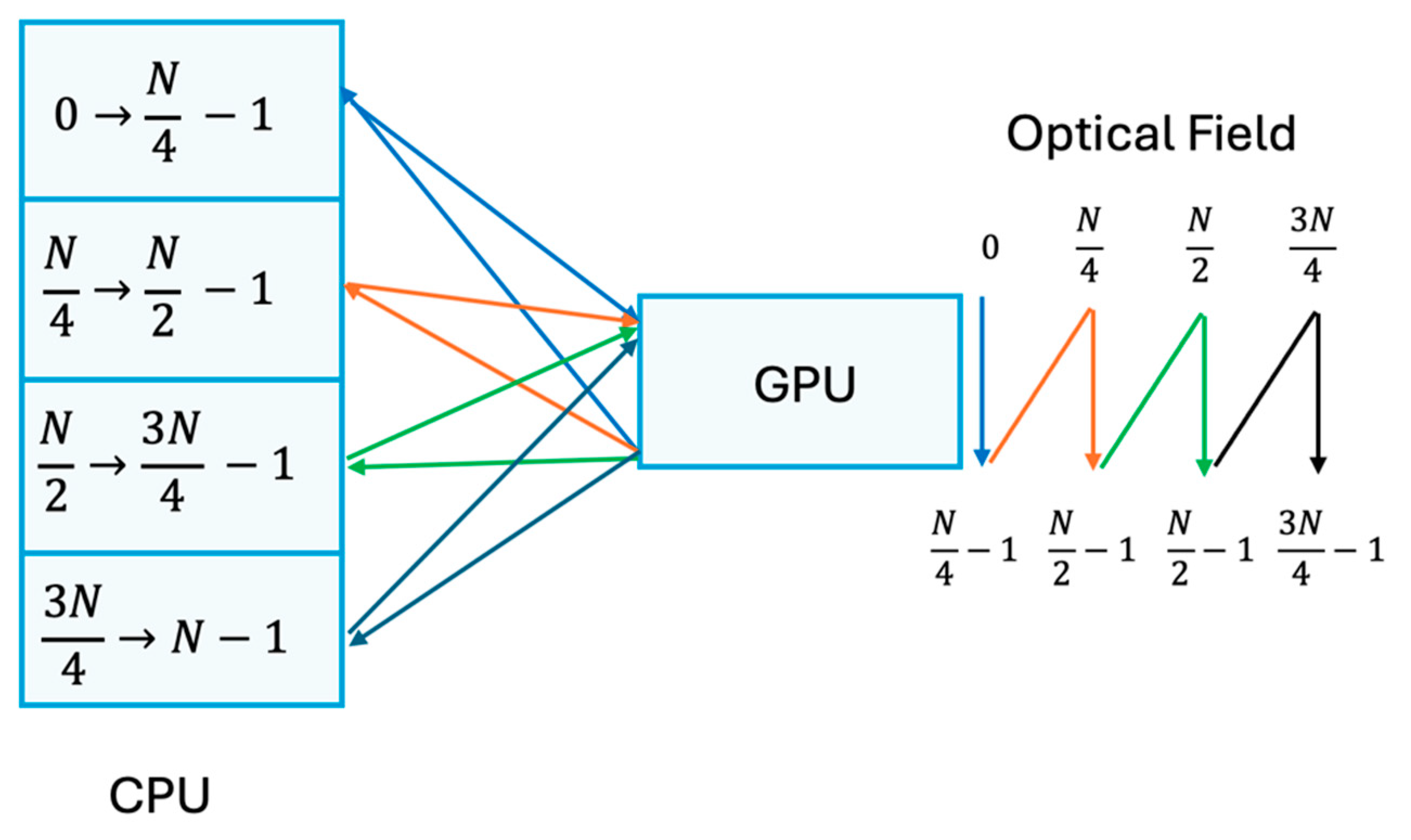
number of batches: The propagation can be split into several longitudinal batches so that the GPU only needs to store the part of the space charge fields required by the current batch. The full three-dimensional space charge field is stored in the CPU. On Google COLAB’s A100 there are 83.5 GB CPU RAM available and 40 GB GPU RAM.
Figure A2.
Diagram of space charge field batching for propagation over N longitudinal steps. For a given time step the complete space charge is stored in CPU. The first quarter of the space charge is loaded into the GPU and optical field is propagated through the corresponding refractive index distribution in the first quarter of the crystal and the first quarter of the space charge is updated by time integration. The updated space charge is returned to the CPU for use in the next time step. The second quarter of the old space charge is then loaded into the GPU and updated together with the optical field and is returned to the CPU for the next time step. The optical field is propagated through the whole crystal as indicated on the left.
fanning study: If selected, spatial frequencies corresponding to the input beam are masked out in the far field so that the amplified scattering can be displayed without saturation by the remnants of the input beam.
use old seeds: Use noise seeds already stored in the prdata dictionary for the current calculation. For example, if comparing static and time dependent fanning distributions. The static case might be run first, its noise seeds saved the dictionary, then reused for a time dependent calculation. If the seeds dictionary is empty, new noise seeds will be generated. The seeds for each run are stored in the run’s dictionary (prdata).
Google drive save folder: When save output is selected, contains the name of the folder on Google Drive where run parameters in the prdata dictionary (saved in the file data.json), output images and movies (for time dependent runs) are stored. If the folder does not exist it will be created.
save output: If selected the run’s data will be stored to disk. It can be retrieved at the beginning of each run instance.
relative dielectric constant: The dielectric constant of the interaction crystal normalized by the permittivity of free space .
mobile charge density: The density of empty sites in the crystal when in the dark with no photorefractive grating. Its units are m
-3. Typical values are of the order of 10
22 m
-3. From Garrett et al[
30]: 6.4 x10
22 m
-3, and from Feinberg et al[
21]: 1.9 x 10
22 m
-3.
temperature K: Temperature in Kelvin.
refractive index: Crystal refractive index. Default is a typical refractive index for BaTiO3 (data available from various sources)
dark intensity: Equivalent optical intensity accounting for thermally ionized carriers. This intensity accounts for dark decay of the gratings. Normalized to the sum of the average peak intensity I0 of the beams. (See appendix B)
Tukey window edge: The edge parameter for the Tukey (cosine taper) window[
31] used to enable absorbing boundaries of the propagation lattice in both real space and Fourier space
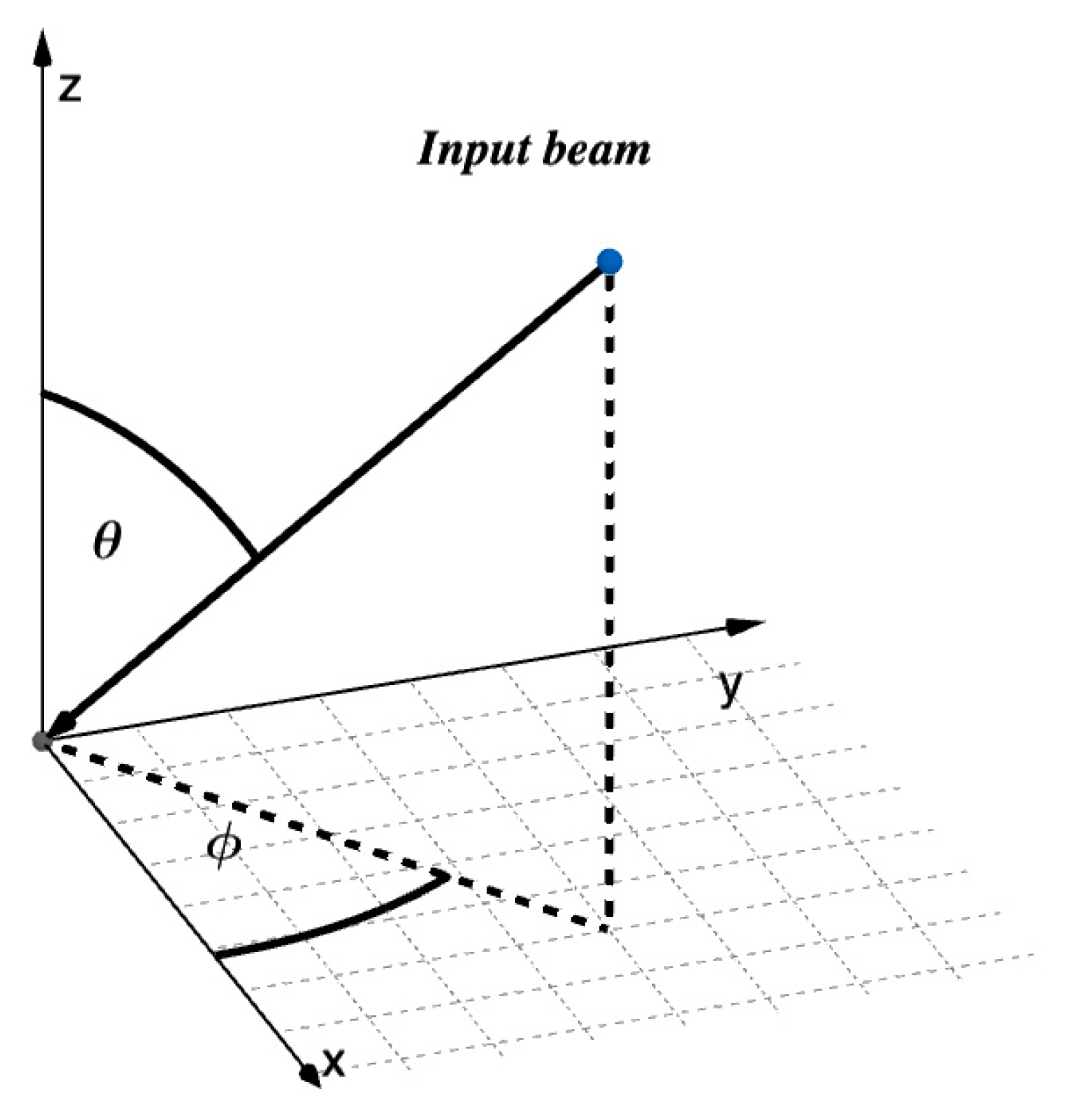
Figure A3.
Physics definitions of polar angle θ and azimuth φ. The transverse plane is xy and the propagation takes place in the z direction.
Figure A3.
Physics definitions of polar angle θ and azimuth φ. The transverse plane is xy and the propagation takes place in the z direction.
Appendix B. The Photorefractive Model
We start with the formulation of the hopping model described in reference [
21]. In this model charge carriers are optically excited and redistributed under the influence of drift and diffusion and produce the space charge fields responsible for the photorefractive effect. The probability that a mobile charge occupies the
nth site is denoted as
Wn. This probability is subject to the following equation which describes the optically induced hopping of carriers into and out of site
n.
where
Dmn is related to the ease with which a carrier can hop from site
m to site
n,
β is the thermal coefficient
e/(
kBT),
e is charge on a single carrier,
kB is Boltzmann’s constant, and
T is the temperature.
ϕmn is the electric potential difference between site
m and site
n,
.
In is the optical intensity at site
n plus the dark intensity
Id. The dark intensity is an empirical effective background intensity accounting for thermal relaxation of the charge distribution. The spacing between sites is assumed to be small enough that we can use a first order expansion of the exponentials:
We next assume that nearest neighbor hopping is dominant, and the sites are equally spaced so that
Dn+1,n =
Dn-1,n =
D so the equation becomes
We now replace the subscripts
n by continuous distance variables
x and let the spacing between sites be denoted as
s.
ϕn+1,n becomes
ϕ (x+s)-
ϕ (s). Second order Taylor expansion about
s then yields:
The site occupation probability
W is proportional to the number density of charge carriers
p so the equation can be rewritten as
We now further simply by writing both
ϕ’ and
p in terms of the electric field, taking advantage of the fact that
ϕ’ is equivalent to
-E, and by using Gauss’s law:
where
pd is the background charge density ensuring that the medium is neutral when all charge carriers are uniformly distributed, and
ε is the dielectric constant.
Following an integration with respect to
x on both sides of the equation, we rewrite it in terms of normalized units to facilitate computation.
where
I is now the local intensity normalized to the average intensity
I0 (usually power
/beam area
e.g. πw02 where
w0 is he beam waist).
E is the electric field normalized to the characteristic space charge field
E0:
Distance
x is normalized to the characteristic distance 1/
k0 where
k0 is
The time
t is normalized to characteristic time units
t =
t0:
A typical value for the characteristic time for the photorefractive material barium titanate is 0.2
seconds with
I0 in units of watts per square centimeter[
21].
When applied to two-beam coupling of plane waves equation as discussed in section 3.1 above, equation (B7), may be approximated as
by retaining only those portions of the space charge field which would be Bragg matched to the beams which produce a grating with wavenumber
kg. This approximation makes clear that the effective time constant for grating buildup is
t0 /(1+
kg2).
Appendix C. Artifacts
Limitations on Step Size
While large values of step sizes
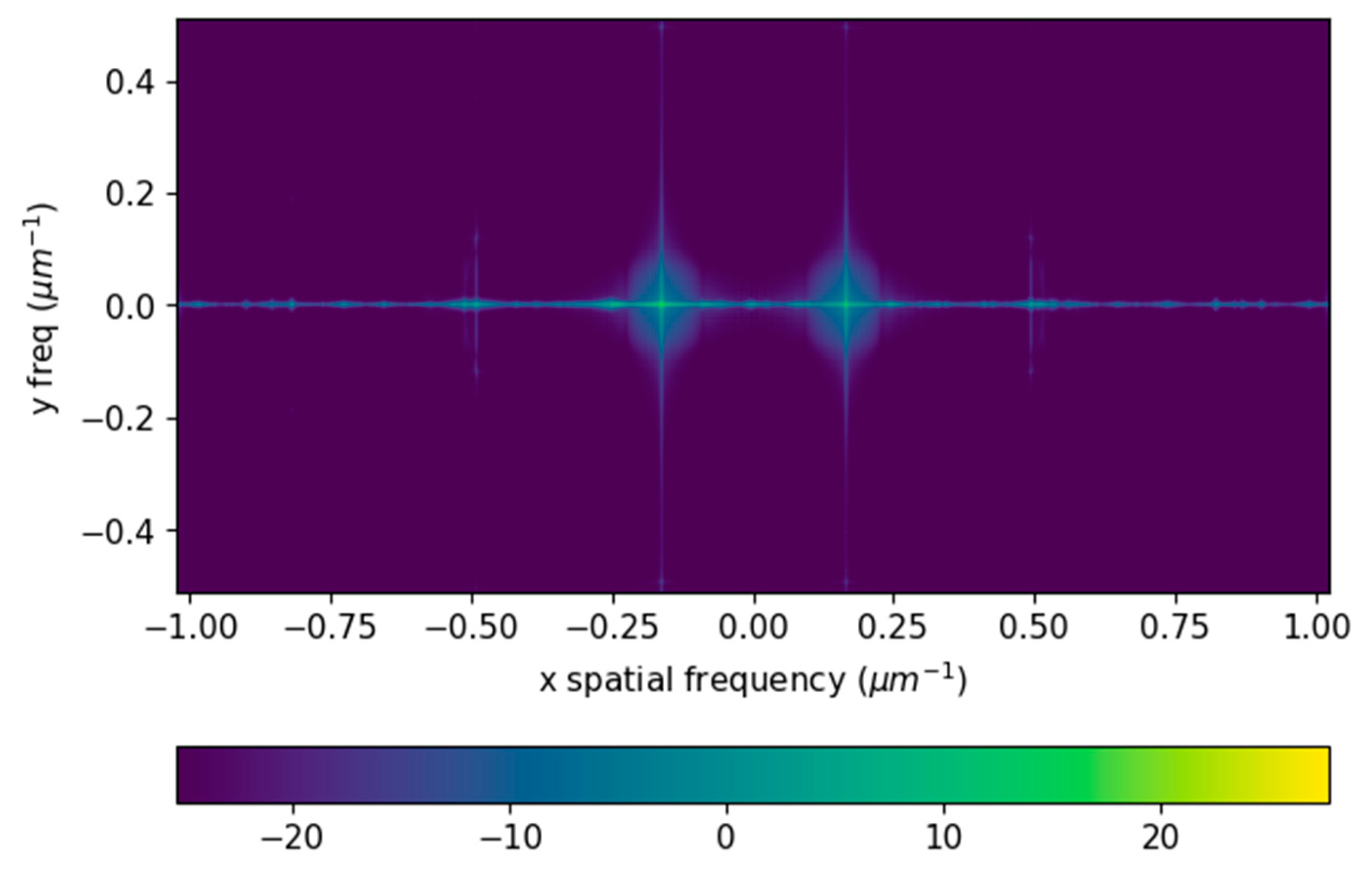
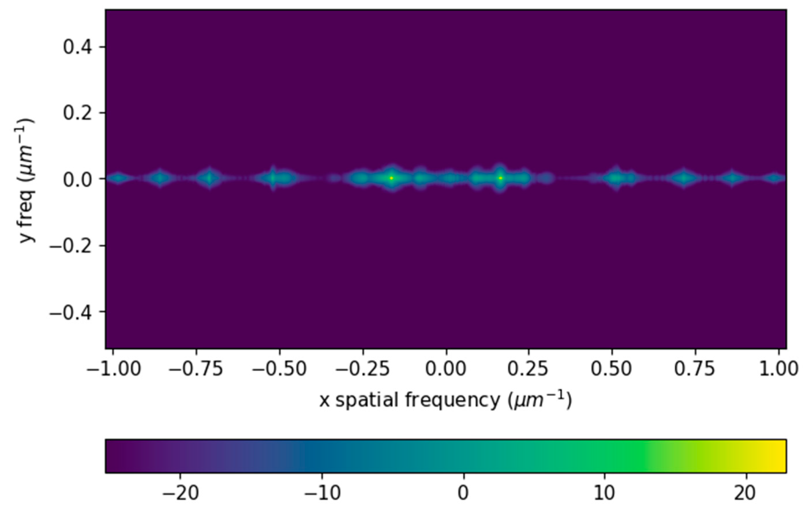
dz can be used for linear propagation, the step size for accurate propagation becomes limited when nonlinear effects are included. This is especially evident when modelling the interaction of image bearing beams with significant spatial complexity or when scattering is included to model amplified scattering (fanning). The model concentrates the photorefractive nonlinearity into planes at the ends of the linear propagation steps creating longitudinal grating artifacts. This grating and its harmonics allow phase matched scattering into directions that are forbidden in spatially continuous interactions. This results in the appearance of the dark rings seen in
Figure A5, as well as other artifacts.
Figure A5.
Computed fanning far field for two different longitudinal step sizes. a) dz = 50μm. The dark rings described in the text can be seen, as well as other artifacts at higher spatial frequencies. Beam waist 200μm, wavelength 0.633μm, x y sampling 8192 x 4096, x y aperture 1 x 1 mm, interaction length 4mm. The color scale maximum is 4 in units of normalized power per unit solid angle. b) Calculation for same parameters except with step size 2μm. The artifacts are eliminated. Color scale maximum here is 6. The fanning efficiency was calculated at 81%.
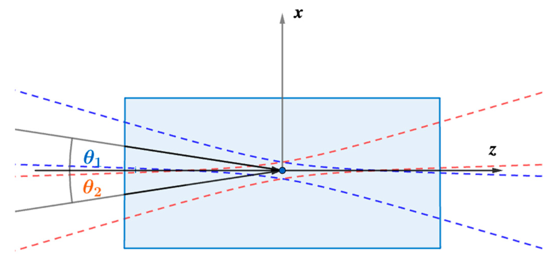
Figure A6 depicts a hypothesis for the process in the
xz plane in the case of fanning generated by a beam with optical wavevector
k0. Fanning results in the development of a broad spectrum of photorefractive gratings. Consider the case of the fundamental component of the longitudinal grating artifact
kz1. The
kg1 component of the fanning grating combines with
kz1 to allow phase matched coupling from the optical wavevector
kf1 into the optical wavevector
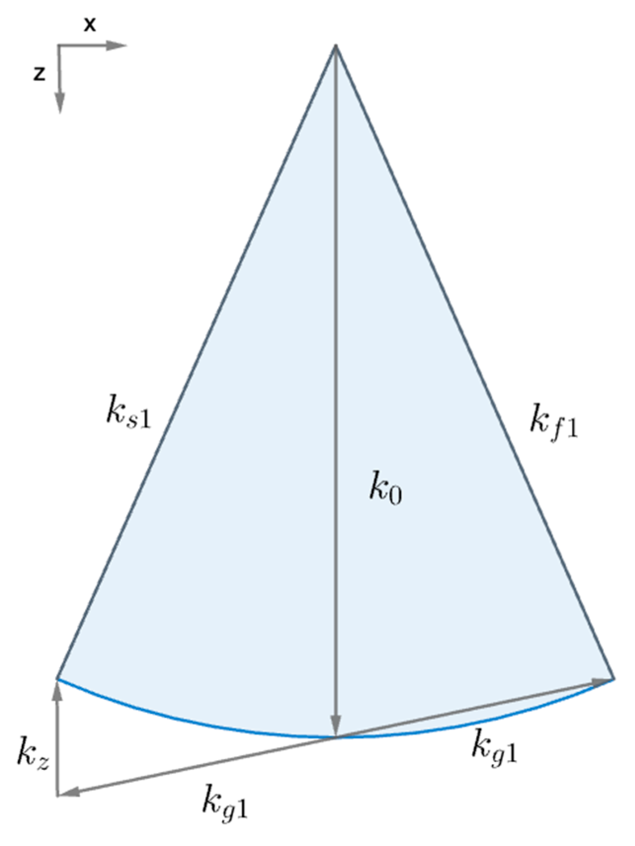
ks1 on the opposite side of the input beam. In three dimensions these phase-matched optical components generalize into an ellipse in the far field. When the beams are incident in the xz plane, the axis lengths of the
jth ring in spatial frequency can be shown to be:
where
θin is the internal propagation angle of the beam in the
xz plane,
n is the refractive index,
j is the order of the harmonic of the longitudinal grating and
λ the wavelength. The bright arcs on the right side of
Figure A5a represent a more serious artifact. These arcs drain a significant amount of power form the true fanning pattern. The physical origin of these artifacts is unknown.
Figure A6.
Hypothesis for the origin of dark amplified scattering rings in split step beam propagation model. A beam with wavevector k0 is incident on the photorefractive crystal. The component of the amplified scattering with wavevector kf1 produced by scattering from the grating component with wavevector kg1 is coupled by that grating and a longitudinal component of the longitudinal grating artifact with wavevector kz into a beam on the opposite side of the incident beam with wavevector ks1. Higher harmonics of the longitudinal grating produce additional higher order rings.
High Order Diffraction
Another effect associated with the longitudinal step size is the appearance of high order diffraction beams. These are generally suppressed by phase mismatch match in the Bragg regime.
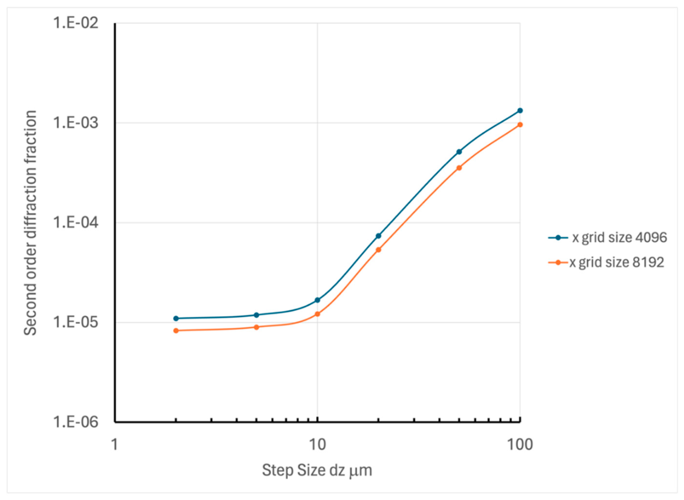
Figure A7 shows that the fraction of input light delivered to second order diffraction in the model is minimized for step sizes less than 7μm where it is about 10
-3 %, rising to only 0.1% for step sizes as large as 100μm. The transverse grid spacing has little influence and only becomes significant for spacings greater than 0.244μm, corresponding to 10 field samples per grating period. An unexpected result is that the low-level high order gratings persist at small step sizes. This effect has been observed before [
14] in the theoretical prediction of ‘kinky beams’.
Figure A7.
Prevalence of second order diffraction in two-beam coupling model for BaTiO3 as a function of longitudinal step size. Beam waists are 400μm, incidence angles 0.1 radians. The wavelength is 488nm. The crystal aperture 2mm x 2mm. Results for two transverse grid sizes are shown: 4096 and 8192 corresponding to transverse grid spacings of 0.488μm and 0.244μm respectively. The grating period is 2.44μm.
References
- Aisawa, S.; Noguchi, K.; Matsumoto, T. Remote Image Classification through Multimode Optical Fiber Using a Neural Network. Optics Letters 1991, 16, 645-647.
- Ancora, D.; Negri, M.; Gianfrate, A.; Trypogeorgos, D.; Dominici, L.; Sanvitto, D.; Ricci-Tersenghi, F.; Leuzzi, L. Low-power multimode-fiber projector outperforms shallow-neural-network. Physical Review Applied 2024, 21. [CrossRef]
- Dudley, J.; Genty, G.; Coen, S. Supercontinuum generation in photonic crystal fiber. Reviews of Modern Physics 2006, 78, 1135-1184. [CrossRef]
- Tegin, U.; Yildirim, M.; Oguz, I.; Moser, C.; Psaltis, D. Scalable optical learning operator. Nature Computational Science 2021, 1, 542-549. [CrossRef]
- Gunter, P.; Huignard, J.P. Photorefractive Materials and Their Applications 1: Basic Effects; Springer: New York, 2005; p. 426.
- Segev, M.; Engin, D.; Yariv, A.; Valley, G.C. Temporal Evolution of Fanning in Photorefractive Materials. Optics Letters 1993, 18, 956-958. [CrossRef]
- Skeldon, M.; Narum, P.; Boyd, R. Non-Frequency-Shifted, High-Fidelity Phase Conjugation with Aberrated Pump Waves by Brillouin-Enhanced 4-Wave-Mixing. Optics Letters 1987, 12, 343-345.
- Lind, R.; Steel, D. Demonstration of the Longitudinal Modes and Aberration-Correction Properties of a Continuous-Wave Dye Laser with a Phase-Conjugate Mirror. Optics Letters 1981, 6, 554-556.
- Feinberg, J.; Hellwarth, R.W. Phase-Conjugating Mirror with Continuous-Wave Gain. Optics Letters 1980, 5, 519-521. [CrossRef]
- White, J.O.; Croningolomb, M.; Fischer, B.; Yariv, A. Coherent Oscillation by Self-Induced Gratings in the Photorefractive Crystal BaTiO3. Applied Physics Letters 1982, 40, 450-452.
- Feinberg, J. Self-Pumped, Continuous-Wave Phase Conjugator Using Internal-Reflection. Optics Letters 1982, 7, 486-488. [CrossRef]
- Cronin-Golomb, M. Whole Beam Method for Photorefractive Nonlinear Optics. Optics Communications 1992, 89, 276-282. [CrossRef]
- Zozulya, A.A.; Saffman, M.; Anderson, D.Z. Propagation of Light-Beams in Photorefractive Media - Fanning, Self-Bending, and Formation of Self-Pumped 4-Wave-Mixing Phase-Conjugation Geometries. Physical Review Letters 1994, 73, 818-821. [CrossRef]
- Brown, W.P.; Valley, G.C. Kinky Beam Paths Inside Photorefractive Crystals. Journal of the Optical Society of America B-Optical Physics 1993, 10, 1901-1906. [CrossRef]
- Ratnam, K.; Banerjee, P.P. Nonlinear Theory of 2-Beam Coupling in a Photorefractive Material. Optics Communications 1994, 107, 522-530. [CrossRef]
- Fainman, Y.; Klancnik, E.; Lee, S.H. Optimal Coherent Image Amplification by 2-Wave Coupling in Photorefractive BaTiO3. Optical Engineering 1986, 25, 228-234. [CrossRef]
- Zozulya, A.A.; Anderson, D.Z. Spatial Structure of Light and a Nonlinear Refractive-Index Generated by Fanning in Photorefractive Media. Physical Review A 1995, 52, 878-881. [CrossRef]
- Horowitz, M.; Kligler, D.; Fischer, B. Time-Dependent Behavior of Photorefractive 2-Wave and 4-Wave-Mixing. Journal of the Optical Society of America B-Optical Physics 1991, 8, 2204-2217. [CrossRef]
- Goodman, J.W. Introduction to Fourier optics, Fourth edition. ed.; W.H. Freeman, Macmillan Learning: New York, 2017; pp. xiv, 546 pages.
- Muys, P. Propagation of vectorial laser beams. Journal of the Optical Society of America B-Optical Physics 2012, 29, 990-996.
- Feinberg, J.; Heiman, D.; Tanguay, A.R.; Hellwarth, R.W. Photorefractive Effects and Light-Induced Charge Migration in Barium-Titanate. Journal of Applied Physics 1980, 51, 1297-1305.
- Vahey, D.W. Nonlinear Coupled-Wave Theory of Holographic Storage in Ferroelectric Materials. Journal of Applied Physics 1975, 46, 3510-3515. [CrossRef]
- Cronin-Golomb, M.; Fischer, B.; White, J.; Yariv, A. Theory and Applications of 4-Wave Mixing in Photorefractive Media. IEEE Journal of Quantum Electronics 1984, 20, 12-30. [CrossRef]
- Kukhtarev, N.V.; Markov, V.B.; Odulov, S.G.; Soskin, M.S.; Vinetskii, V.L. Holographic Storage in Electrooptic Crystals .1. Steady-State. Ferroelectrics 1979, 22, 949-960.
- Feinberg, J. Asymmetric Self-Defocusing of an Optical Beam from the Photorefractive Effect. Journal of the Optical Society of America 1982, 72, 46-51. [CrossRef]
- Montemezzani, G.; Zozulya, A.A.; Czaia, L.; Anderson, D.Z.; Zgonik, M.; Gunter, P. Origin of the Lobe Structure in Photorefractive Beam Fanning. Physical Review A 1995, 52, 1791-1794. [CrossRef]
- Vachss, F. An Analytic Expression for the Photorefractive Two Beam Coupling Response Time. In Proceedings of the Topical Meeting on Photorefractive Materials, Effects, and Devices II, Aussois, 1990/01/17, 1990; p. BP8.
- Iserles, A. A First Course in the Numerical Analysis of Differential Equations, Second ed.; Cambridge University Press: Cambridge, 2009.
- PARSHALL, E.; CRONIN-GOLOMB, M.; BARAKAT, R. Model of Amplified Scattering in Photorefractive Media - Comparison of Numerical Results and Experiment. Optics Letters 1995, 20, 432-434. [CrossRef]
- Garrett, M.H.; Chang, J.Y.; Jenssen, H.P.; Warde, C. High Beam-Coupling Gain and Deep-Trap and Shallow-Trap Effects in Cobalt-Doped Barium-Titanate, BaTiO3-Co. Journal of the Optical Society of America B-Optical Physics 1992, 9, 1407-1415. [CrossRef]
- Harris, F.J. Use of Windows for Harmonic-Analysis with Discrete Fourier-Transform. Proceedings of the Ieee 1978, 66, 51-83. [CrossRef]
|
Disclaimer/Publisher’s Note: The statements, opinions and data contained in all publications are solely those of the individual author(s) and contributor(s) and not of MDPI and/or the editor(s). MDPI and/or the editor(s) disclaim responsibility for any injury to people or property resulting from any ideas, methods, instructions or products referred to in the content. |
© 2025 by the authors. Licensee MDPI, Basel, Switzerland. This article is an open access article distributed under the terms and conditions of the Creative Commons Attribution (CC BY) license (http://creativecommons.org/licenses/by/4.0/).