Application of the Hill-Wheeler Formula in Statistical Models of Nuclear Fission: A Statistical Mechanical Approach Based on Similarities with Semiconductor Physics

Hirokazu Maruyama

doi:10.20944/preprints202412.2335.v1

Submitted:

26 December 2024

Posted:

27 December 2024

You are already at the latest version

Abstract

This study proposes a novel theoretical approach to understanding the statistical mechanical similarities between nuclear fission phenomena and semiconductor physics. Using the Hill-Wheeler formula as a quantum mechanical distribution function and establishing its correspondence with the Fermi-Dirac distribution function, we analyzed nuclear fission processes for nine nuclides (232Th, 233U, 235U, 238U, 237Np, 239Pu, 240Pu, 242Pu, 241Am) using JENDL-5.0 data.

Keywords:

nuclear fission

;

statistical model

;

Hill-Wheeler equation

;

quantum mechanical distribution function

;

distribution function

;

fission yield

;

scission distance

;

selective channel scission model

;

effective fission barrier correction

;

nuclear deformation

;

fission cross-section

Subject:

Physical Sciences - Condensed Matter Physics

Introduction

Since its discovery by Hahn and Strassmann in 1938, nuclear fission has remained a central research topic in nuclear physics. While phenomenological understanding has advanced through liquid drop models and shell corrections, the statistical mechanical foundation of nuclear fission remains incompletely understood.

In particular, while experimental data on fission product yield distributions has accumulated, theoretical prediction remains challenging. Even for major fission reactions in nuclear reactors, such as ²³⁵U and ²³⁹Pu, a complete theoretical description of mass and charge distributions remains elusive.

Meanwhile, in semiconductor physics, the description of electronic states based on Fermi-Dirac statistics has been highly successful. In particular, phenomena such as band gaps and carrier transport are precisely understood through statistical mechanical approaches using the Fermi-Dirac distribution function.

This research proposes a novel theoretical approach based on the insight that there might exist statistical mechanical similarities between nuclear fission phenomena and semiconductor physics, which appear to be completely different physical systems. Specifically, we reinterpret the Hill-Wheeler formula as a quantum mechanical extension of the Fermi-Dirac distribution function and attempt to provide a statistical mechanical description of nuclear fission phenomena.

The characteristics of this approach are:

Reinterpretation of the Hill-Wheeler formula as a quantum mechanical distribution function for nuclear fission
Establishment of a systematic method to determine the Fermi energy for fission fragments
Presentation of a statistical mechanical interpretation of prompt neutron spectra

The structure of this paper is as follows. Section 2 presents an overview of the statistical mechanical nuclear fission model, and Section 3 explains the specific calculation method using the Hill-Wheeler formula.Section 4 presents calculation results and discusses their physical significance, while Section 5 discusses the similarities between neutron spectra and semiconductor physics. Finally, Section 6 presents conclusions and future prospects.

This study is a substantially revised and academically reorganized version of the authors’ previously published works [1,2]. In the earlier publications,

E_{x}

was interpreted as the excitation energy; however, in this paper,

E_{x}

is redefined as the Fermi energy, prompting a fundamental overhaul of both the theoretical framework and the numerical analysis approach. Specifically, new insights have been gained into the energy spectrum and cross-section analyses within the statistical model of nuclear fission. Another notable feature of this work is the expansion toward a more versatile numerical method, achieved by utilizing the optimization results obtained under Mathematica ver.11.2 and performing additional analyses and visualizations in the latest version (ver.14.1). In this paper, we also revisit the theoretical background that was not thoroughly addressed in the previous works [1,2], and discuss the physical implications of the analyses carried out using the newly redefined

E_{x}

. Through this approach, we aim to establish a new foundation for understanding fission phenomena from perspectives that were not addressed in earlier interpretations.

Overview of Statistical Mechanical Nuclear Fission Model

While various approaches have been proposed for the theoretical description of nuclear fission phenomena, many require complex parameter adjustments. Among these, the Selective Channel Scission (SCS) model, which forms the basis of this research, is noteworthy for its ability to predict fission yields with minimal parameters.

Basic Framework of the Selective Channel Scission Model

The SCS model, proposed by Takahashi, Ohta, et al. in 2001, calculates yields by decomposing the nuclear fission process into individual channels and determining the fission barrier

E_{f i}

for each channel[3,4,5,6,7,8]. At the core of this model is the Hill-Wheeler formula:

\begin{matrix} f (E) = \frac{1}{1 + e x p [\frac{2 π Δ E}{ℏ ω_{f}}]}, \end{matrix}

(1)

where the energy difference

Δ E_{i}

is defined as:

\begin{matrix} Δ E_{i} = E_{f i} - E_{x}, \end{matrix}

(2)

leading to the transmission probability:

\begin{matrix} T_{i} (E_{x}) \approx \frac{1}{1 + e x p [- 0.218 κ \sqrt{μ_{m}} Δ E_{i}]}, \end{matrix}

(3)

Introduction of Statistical Mechanical Interpretation

In this research, we propose a new statistical mechanical interpretation of the Hill-Wheeler formula in the SCS model. Specifically, we reinterpret Equation (1) as a quantum statistical mechanical distribution function for nuclear fission, introducing the following correspondences:

$E_{x}$ : Corresponds to Fermi energy (chemical potential)
$E_{f i}$ : Fission Barrier
$\frac{ℏ ω_{f}}{2 π}$ : Quantum statistical mechanical temperature energy (corresponding to $k T$ )

Based on this interpretation, systematic analysis using JENDL-5.0 nuclear fission yield data revealed the following important findings:

The effective nuclear fission distance ( $R_{e f f}$ ) is proportional to the product of the charges of the fission fragments $(Z) (Z_{p a r e n t} - Z)$
The effective fission distance shows maximum values in the symmetric fission region ( $Z = Z_{p a r e n t} / 2$ ) at the atomic nuclear scale (approximately 1 fm)
The Fermi energy distribution has values unique to each fission fragment, with maximum values consistent with fission barrier energies

Calculation Using the Hill-Wheeler Formula in Nuclear Fission Statistical Model

Here we present the calculation conditions, results, and equations.

Calculation Conditions

The experimental data and target nuclei used in the calculations are as follows:

Table 1. Nine target nuclei and calculation conditions used in this study.

Target	Neutron	Incident Neutron	Average Number of Prompt
Nucleus	Separation Energy	Energy	Neutrons (0.0253eV/500keV/14MeV)
${}^{232}{Th}$ +n	4.7863 MeV	500keV, 14MeV	-/2.198/4.402
${}^{233}U$ +n	6.8455 MeV	0.0253eV, 500keV, 14MeV	2.497/2.933/4.521
${}^{235}U$ +n	6.5455 MeV	0.0253eV, 500keV, 14MeV	2.437/2.879/4.378
${}^{238}U$ +n	4.8063 MeV	500keV, 14MeV	-/2.579/4.458
${}^{237}{Np}$ +n	5.4882 MeV	0.0253eV, 500keV, 14MeV	2.683/2.788/4.401
${}^{239}{Pu}$ +n	6.5342 MeV	0.0253eV, 500keV, 14MeV	2.875/3.242/4.891
${}^{240}{Pu}$ +n	5.2415 MeV	0.0253eV, 500keV, 14MeV	2.860/3.236/4.893
${}^{242}{Pu}$ +n	5.0336 MeV	0.0253eV, 500keV, 14MeV	2.936/3.276/4.921
${}^{241}{Am}$ +n	5.5287 MeV	0.0253eV, 500keV, 14MeV	3.209/3.453/4.972

It is noteworthy that this statistical model requires only the experimental data of fission product charge distribution yields, neutron separation energy, incident neutron kinetic energy, and average number of prompt neutrons. No adjustable parameters are needed.

Reasons for Considering the Hill-Wheeler Formula as Nuclear Fission’s Quantum Mechanical Distribution Function

The charge and mass distributions of fission products show consistent yield curves across experiments, indicating that nuclear fission follows mathematical physical laws. This law must be a distribution function following statistical mechanics. The validity of this assumption is confirmed later by showing that neutron spectra is proportional to the density of states × Fermi-Dirac distribution function.

Let us examine three types of distribution functions used in statistical mechanics:

The Maxwell-Boltzmann distribution function for classical particles:

\begin{matrix} f (E) = \frac{1}{e x p [\frac{Δ E}{k t}]}, \end{matrix}

(4)

The Bose-Einstein distribution function for bosons:

\begin{matrix} f (E) = \frac{1}{- 1 + e x p [\frac{Δ E}{k t}]}, \end{matrix}

(5)

And the Fermi-Dirac distribution function for fermions:

\begin{matrix} f (E) = \frac{1}{1 + e x p [\frac{Δ E}{k t}]}, \end{matrix}

(6)

where

Δ E = E - E_{F}

, and

E_{F}

is the Fermi energy (chemical potential).

When applying statistical mechanics to atomic nuclei, the basic model is the Fermi gas model, which uses Equation (6) as its distribution function. However, this model can theoretically explain only limited aspects of experimental data.

Therefore, instead of the Fermi-Dirac distribution function, we used the Hill-Wheeler formula, which D.L. Hill and J.A. Wheeler derived assuming a harmonic oscillator:

\begin{matrix} f (E) = \frac{1}{1 + e x p [\frac{2 π Δ E}{ℏ ω_{f}}]}, \end{matrix}

(7)

as the distribution function for nuclear fission.

The reason for this assumption is that Equation (7) has the same form as the distribution function in Equation (6). Although they differ in nomenclature (distribution function versus transmission probability), both equations calculate probability from energy, effectively performing the same function.

Comparing Equations (6) and (7), we see that ℏ (Planck’s constant) corresponds to k (Boltzmann constant), both being constants. Furthermore,

ω_{f}

corresponds to t, both being quantities that increase with energy. While the equations appear different, we consider them essentially the same, with the quantum mechanical value

ℏ ω_{f} / 2 π

replacing the temperature energy

k t

.

More boldly stated, we consider "the Hill-Wheeler Formula (7) to be a more fundamental quantum mechanical distribution function than the Fermi-Dirac distribution function (6)."

The reasons are:

Temperature energy $k t$ does not exist for a single atomic nucleus or molecule. While one might argue that the Fermi-Dirac distribution function is used in statistical mechanics where vast numbers of atoms or molecules exist, there should be no problem with having a more fundamental distribution function that replaces $k t$ with $ℏ ω_{f} / 2 π$ and is applicable even to single atoms.
When considering a quantum mechanically simpler form of Equation (6), it seems unlikely that any form other than (7) could exist.

However, these are intuitive reasons. We need to verify this through actual calculations, which we will demonstrate in this paper.

As a side note, if Fermions follow Equation (7), then the quantum mechanical advanced version of the Bose-Einstein distribution function for Bosons would be:

\begin{matrix} f (E) = \frac{1}{- 1 + e x p [\frac{2 π Δ E}{ℏ ω_{f}}]}, \end{matrix}

(8)

Derivation of the Nuclear Fission Statistical Model

Here we derive the equations for the nuclear fission statistical model from the Hill-Wheeler Formula (7), which we consider to be an advanced version of the distribution function.

Since Equation (7) was derived assuming a harmonic oscillator, we maintain this assumption. We consider the atomic nucleus as a harmonic oscillator where fission fragments (FP1 and FP2) are connected by an ideal spring, as shown in Figure 1. (Since we are dealing with charge distribution experimental data, we use charges Z1, Z2 rather than masses for the fission fragment harmonic oscillator.)

Restating the Hill-Wheeler formula:

\begin{matrix} f (E) = \frac{1}{1 + e x p [\frac{2 π Δ E}{ℏ ω_{f}}]}, \end{matrix}

(9)

This equation was derived by Hill and Wheeler from the Schrödinger equation assuming a harmonic oscillator[11,12,13], where the harmonic oscillator potential is:

\begin{matrix} V (r) = V_{0} - \frac{1}{2} μ_{z} {ω_{f}}^{2} r^{2}, \end{matrix}

(10)

The

ω_{f}

in the denominator is the angular frequency of the harmonic oscillator, and with

k_{f}

as the force constant:

\begin{matrix} ω_{f} = 2 π ν = 2 π \sqrt{\frac{k_{f}}{μ_{z}}}, \end{matrix}

(11)

The reduced mass

μ_{Z}

uses charges Z1, Z2 as shown in Figure 1:

\begin{matrix} μ_{Z} = \frac{Z 1 * Z 2}{(Z 1 + Z 2)}, \end{matrix}

(12)

Thus, Equation (9) becomes:

\begin{matrix} f (E) = \frac{1}{1 + e x p [\frac{2 π Δ E}{ℏ \sqrt{\frac{k_{f}}{μ_{z}}}}]}, \end{matrix}

(13)

Since

\sqrt{μ_{Z}}

is the product of charges Z1, Z2 according to Equation (12) and describes a parabola, setting its maximum value as

\sqrt{μ_{Z m a x}}

:

\begin{matrix} \sqrt{μ_{Z}} = \sqrt{μ_{Z m a x}} * \sqrt{\frac{μ_{Z}}{μ_{Z m a x}}}, \end{matrix}

(14)

Then:

\begin{matrix} f (E) = \frac{1}{1 + e x p [\frac{2 π \sqrt{\frac{μ_{Z}}{μ_{Z m a x}}} Δ E}{ℏ \sqrt{\frac{k_{f}}{μ_{z m a x}}}}]}, \end{matrix}

(15)

Let us compare this with the Fermi-Dirac distribution function (restating Equation (6)):

\begin{matrix} f (E) = \frac{1}{1 + e x p [\frac{Δ E}{k t}]}, \end{matrix}

(16)

The value corresponding to

k t

in the Fermi-Dirac distribution function (16) is

ℏ \sqrt{\frac{k_{f}}{μ_{z m a x}}}

in Equation (15). Considering what corresponds to this temperature energy

k t

, we propose it is the incident neutron energy. The reason is that just as the distribution state in a container (solid, semiconductor, etc.) changes with temperature energy

k t

in the Fermi-Dirac distribution function (16), similarly, the distribution state in the container (atomic nucleus) changes with incident neutron energy in distribution function (15).

Therefore, with

S n

= neutron separation energy and

K n

= neutron kinetic energy:

\begin{matrix} ℏ \sqrt{\frac{k_{f}}{μ_{z m a x}}} = S n + K n, \end{matrix}

(17)

This leads to:

\begin{matrix} f (E) = \frac{1}{1 + e x p [\frac{2 π \sqrt{\frac{μ_{Z}}{μ_{Z m a x}}} Δ E}{S n + k n}]}, \end{matrix}

(18)

Here,

Δ E

is considered as the difference between

E_{f i}

(fission barrier energies of fission fragments) and

E_{x}

(Fermi energy):

\begin{matrix} Δ E_{i} = E_{f i} - E_{x}, \end{matrix}

(19)

In our nuclear fission calculations, both

E_{x}

(which becomes Fermi energy) and

E_{f i}

vary with the elements constituting nuclear matter (we will later change

E_{x}

to

E_{x i}

). The calculation of

E_{f i}

will be explained in the next section, and the variation of

E_{x}

will be discussed in later considerations.

Thus, the final statistical model equation using the Hill-Wheeler formula becomes:

\begin{matrix} f_{i} (E) = \frac{1}{1 + e x p [\frac{2 π \sqrt{\frac{μ_{Z}}{μ_{Z m a x}}} Δ E_{i}}{S n + k n}]}, \end{matrix}

(20)

Calculation Process from Nuclear Fission Statistical Model to Charge Distribution

Here we show the calculation process for obtaining charge distribution using Equation (20) derived from the Hill-Wheeler formula.

Near the potential barrier peak shown in Figure 2, various numerical calculations have been attempted, but no definitive method exists. Currently, it is thought that shell effects may form multiple barriers, but in our case, the nuclear Fermi energy obtained for each fission fragment will have different values, ultimately showing a structure that forms fission isomers. However, for calculation purposes, we assume a single-barrier structure.

The validity of this assumption is demonstrated by later calculation results showing that the fission energy used in calculating charge distribution is predominantly due to the Coulomb force between two fission fragments, with nuclear force effects being comparatively small, making the single-barrier assumption acceptable.

To reiterate, while the potential strictly forms multiple barriers, since the dominant contribution comes from the Coulomb force between two fission fragments, treating it as a single barrier with small perturbations is justified.

As shown in Figure 2, when two fission fragments are separated sufficiently far apart, the potential equals the Coulomb potential. Therefore, we assume that fission occurs at the internuclear distance where the bare fragment Coulomb potential corresponds to the channel-dependent fission barrier. We call this internuclear distance the effective fission distance

R_{e f f}

, and define it using fission parameters

k 1

and

k 2

as follows:

\begin{matrix} R_{e f f} ≒ k 1 * (Z 1 * Z 2 + k 2), \end{matrix}

(21)

where

Z 1

and

Z 2

are the charges of the fission fragments after fission.

The reason for introducing these fission parameters

k 1

and

k 2

is that through the deformation process leading to fission, the nuclear shape at the time of fission is expected to elongate in proportion to the charges

Z 1

and

Z 2

of the spherical fission fragments, as shown in Figure 2. Therefore, the distance between fission fragments, accounting for this elongation, should be proportional to the product of fragment charges

Z 1 * Z 2

with parameters

k 1

and

k 2

considered. These parameters

k 1

and

k 2

can be automatically calculated from experimental data and do not need to be determined manually.

The channel-dependent fission barrier

E_{f i}

is determined by subtracting the Q-value for each fission reaction from the value of the interfragment Coulomb potential (effective Coulomb energy) at the effective fission distance

R_{e f f}

:

\begin{matrix} E_{f i} = E_{c}^{'} - Q, \end{matrix}

(22)

The first term on the right side, the Coulomb potential

E_{c}^{'}

, is:

\begin{matrix} E_{c}^{'} = 1.44 * Z 1 * Z 2 / R_{e f f}, \end{matrix}

(23)

These calculation Formulas (22) and (23) are the same as in the SCS model[8,9,10,11,12,13].

Finally, the charge distribution yields of each fission product are calculated by substituting these values into the nuclear fission statistical model Equation (20) for each fission reaction and then computing:

\begin{matrix} T_{i} (E_{x i}) = \frac{\sum_{j} f_{i} (E_{x i}^{j})}{\sum_{j} f_{i} (E_{x i}^{j}) + \sum_{j} f_{i} (E_{x i + 1}^{j}) + . . . . . .}, \end{matrix}

(24)

Here,

\sum_{j} f_{i} (E_{x i}^{j})

means summing over all possible isotopes (denoted by subscript j) of the fission fragments that can be produced in nuclear fission. For example, in the case of atomic number i=56 (

{}_{56}{Ba}

), this would mean summing all possible values for fission products from

{}_{56}^{114}{Ba}

to

{}_{56}^{153}{Ba}

.

Specific Calculations

In this study, we used charge distribution experimental data as calculation data, i.e., calculation conditions, and performed the following three calculations using the nuclear fission statistical model:

Calculation of Fission Distance Between Two Fission Fragments

In Equation (19), $Δ E_{i} = E_{f i} - E_{x}$ , we set the Fermi energy $E_{x} = 0$ and solved for the fission distance $R_{e f f}$ in Equation (21) as an unknown variable within Equation (20). As shown in Figure 4, the results showed that the fission distance is proportional to the charges Z of the two fission fragments. Specifically, it is proportional to Z*(atomic number-Z)=Z*atomic number- $Z^{2}$ .

Furthermore, these results showed that this distance distributes within the range of approximately 1.0-1.2 fm. This agrees with values predicted by other theories.
Calculation of Charge Distribution for Zero Fermi Energy (Ground State)

Using the fission distance $R_{e f f}$ obtained in step 1 above, we calculated theoretical values for charge distribution using Equation (20) with Fermi energy $E_{x} = 0$ (ground state) in Equation (19), $Δ E_{i} = E_{f i} - E_{x}$ . Figure 5 shows a comparison between theoretical values and experimental data. As can be seen from the figure, even with Fermi energy $E_{x} = 0$ , theoretical values closely match experimental data.
Calculation of Fermi Energy for Each Fission Fragment

First, we modified Equation (19), $Δ E_{i} = E_{f i} - E_{x}$ to $Δ E_{i} = E_{f i} - E_{x i}$ , assuming the existence of different Fermi energies $E_{x i}$ for different channels. Then, using the fission distance $R_{e f f}$ obtained above, we solved for this $E_{x i}$ as an unknown variable by solving simultaneous equations for all possible patterns of compound nucleus splitting into two fission fragments to obtain the nuclear fission yield charge distribution. As shown in Figure 6, this resulted in obtaining Fermi energies $E_{x i}$ with different values for each element (fission fragment) constituting the compound nucleus.

For detailed calculations, please refer to the attached Mathematica code.

Results and Discussion

In this section, we discuss the physical meaning and theoretical interpretation of the calculation results presented in the previous section.

Physical Significance of Effective Fission Distance Between Fragments

As a representative example, Figure 4 shows the calculation results for

{}^{235}U

.

For

{}^{235}U

, the effective fission distance

R_{e f f}

is expressed as:

\begin{matrix} R_{e f f} = - 0.517291 + 0.000824625 (92.0016 - Z) Z [f m] \end{matrix}

Similar analyses were conducted for the other eight nuclides, all showing similar quadratic dependence:

\begin{matrix} {}_{90}^{232}{Th} e f f e c t i v e f i s s i o n d i s t a n c e (500 k e V) \\ R_{e f f} = - 0.457368 + 0.000812599 (89.9987 - Z) Z \\ {}_{90}^{232}U e f f e c t i v e f i s s i o n d i s t a n c e (500 k e V) \\ R_{e f f} = - 0.362683 + 0.000727996 (92.9985 - Z) Z \\ {}_{92}^{235}U e f f e c t i v e f i s s i o n d i s t a n c e (0.0253 e V) \\ R_{e f f} = - 0.517291 + 0.000824625 (92.0016 - Z) Z \\ {}_{92}^{238}U e f f e c t i v e f i s s i o n d i s t a n c e (500 k e V) \\ R_{e f f} = - 0.339285 + 0.000731257 (92.0027 - Z) Z \\ {}_{93}^{237}{Np} e f f e c t i v e f i s s i o n d i s t a n c e (0.0253 e V) \\ R_{e f f} = - 0.364831 + 0.000729022 (92.995 - Z) Z \\ {}_{94}^{239}{Pu} e f f e c t i v e f i s s i o n d i s t a n c e (0.0253 e V) \\ R_{e f f} = - 0.405216 + 0.000732862 (94.0015 - Z) Z \\ {}_{94}^{240}{Pu} e f f e c t i v e f i s s i o n d i s t a n c e (0.0253 e V) \\ R_{e f f} = - 0.396877 + 0.000729146 (93.9991 - Z) Z \\ {}_{94}^{242}{Pu} e f f e c t i v e f i s s i o n d i s t a n c e (0.0253 e V) \\ R_{e f f} = - 0.410242 + 0.000734583 (94.004 - Z) Z \\ {}_{95}^{241}{Am} e f f e c t i v e f i s s i o n d i s t a n c e (0.0253 e V) \\ R_{e f f} = - 0.466525 + 0.000744743 (95.0044 - Z) Z \end{matrix}

From these results, the following important characteristics have emerged:

1. For all nuclides, the effective fission distance is proportional to the product of fragment charges 2. The proportionality coefficient is nearly constant across nuclides (range: 0.000727-0.000825) 3. Maximum values appear in regions where each nuclide’s charges are nearly symmetric 4. The obtained effective fission distances are on the scale of atomic nuclear size (approximately 1.0-1.2 fm)

This charge dependence is thought to reflect the collective motion of nucleons during the fission process. In particular, the convergence of the proportionality coefficient to a narrow range suggests the existence of a universal characteristic in the fission mechanism.

These calculation results show that when the product of fragment charges Z1 and Z2 (atomic number-Z1) is maximum, the Coulomb repulsion force reaches its maximum value, and the nuclear fission distance becomes maximum. This value was derived as a result of calculating the fission distance

R_{e f f}

as an unknown variable, but it agrees with the intuitive image of nuclear fission.

It is difficult to imagine that the distance at nuclear fission would be independent of charges Z1 and Z2. Although the exact process of nuclear fission cannot currently be confirmed experimentally, it is most natural and consistent with intuition to consider that it is proportional to the product of fragment charges Z1 and Z2, as shown in Figure 1.

Moreover, the calculation results show that the fission distance

R_{e f f}

is approximately 1.0-1.2 fm. While nuclear force potential values cannot be directly determined experimentally, calculations using Woods-Saxon potential models and QCD lattice theory also indicate that nuclear forces weaken rapidly beyond a radius of about 1 fm[12].

This result does not contradict the finding that the fission distance

R_{e f f}

is approximately 1.0-1.2 fm. It suggests that nuclear fission occurs when nuclear forces weaken around 1.2 fm, and Coulomb repulsion between fragments becomes dominant.

As described above, for all nine analyzed nuclides, we found that the fission distance is proportional to the product of fragment charges Z1 and Z2, and

R_{e f f}

is approximately 1.0-1.2 fm. It is unlikely that such simple results would emerge by chance. Therefore, we consider this to be one piece of evidence supporting the validity of our nuclear fission statistical model (20), which assumes the Hill-Wheeler Formula (7) as the distribution function for nuclear fission.

Significance of Charge Distribution Reproduction in Ground State

Figure 5 shows a representative example for

{}^{235}U

.

In this study, we revealed the state of nuclear fission Fermi energy through the following analysis process:

First, using nuclear fission yield charge distribution experimental data from JENDL-5, we calculated the effective distance between fission fragments (

R_{e f f}

). This revealed that this distance is proportional to the product of the charges of the two fission fragments. This proportional relationship was confirmed to hold for all analyzed nuclides.

Next, using the obtained effective distance, we derived theoretical curves using the Hill-Wheeler formula and performed fitting with experimental data. By taking the difference between the fitted values and those predicted by the original theoretical equation, we quantitatively determined the unique energy states possessed by each fission fragment.

In this analysis process, the correction values obtained through fitting represent the Fermi energies of each fission fragment.

Specifically, we calculated the Fermi energy

E_{x}

of each fission fragment from the difference

Δ E

between the fission fragment’s energy level

E_{f i}

and the correction value (

E_{x} = E_{f i} - Δ E

).

A particularly noteworthy point is that, as shown in Figure 5, the charge distribution observed experimentally can be reproduced almost perfectly even when this Fermi energy is set to zero. This discovery provides the important insight that nuclear fission is primarily driven by the nucleus’s internal energy (Coulomb force between the two fragments), and the Fermi energy required for fission is surprisingly small compared to this self-energy.

Inhomogeneity of Fermi Energy Distribution

Figure 6 shows the relationship between Fermi energy distribution and charge distribution for

{}^{235}U

as a representative example.

From these calculation results, the following important characteristics of Fermi energy during nuclear fission have been revealed:

1. Fermi energy is not uniform across the entire nucleus but strongly depends on the fission fragment’s charge number 2. Its distribution shows close correlation with the charge distribution 3. The maximum values are comparable to fission barrier energies

A particularly noteworthy point is that these results show remarkable similarities with semiconductor physics. In semiconductors, it is known that the Fermi energy is approximately half the value of the band gap energy (for example, for Si with a band gap of 1.1eV, the Fermi energy is about 0.5eV). Similarly, in our calculations, the nuclear fission Fermi energy was found to be about 0.5-0.9 times the predicted fission barrier energy.

Fermi Energy and Fission Barrier

Table 2 shows a comparison between the maximum values of Fermi energy obtained from our nuclear fission statistical model and the generally predicted fission barrier energies.

This comparison has revealed important physical insights.

For

{}^{235}U

, the average value of the calculated Fermi energy is 3.85 MeV, which is approximately 0.65 times the predicted fission barrier energy of 5.8-6.0 MeV. Similar ratios are observed for other nuclides, with calculated Fermi energies typically ranging from 0.5 to 0.9 times the predicted barrier energies.

For

{}^{239}{Pu}

and

{}^{240}{Pu}

, the average values of calculated Fermi energies (4.36 MeV and 4.90 MeV respectively) are about 0.74-0.82 times the predicted fission barrier energies (5.9-6.0 MeV), showing ratios similar to those observed in the relationship between band gap and Fermi energy in semiconductors.

However, for

{}^{242}{Pu}

, the calculated average Fermi energy (6.38 MeV) exceeds the predicted fission barrier energy (about 6.0-6.2 MeV). This exceptional behavior might be attributed to the unique nuclear structure of

{}^{242}{Pu}

and requires further investigation.

The variation of Fermi energy with incident neutron energy also provides important insights. The calculation results for three energy regions - 0.0253eV, 500keV, and 14MeV - show systematic changes for many nuclides. For example, in

{}^{235}U

, the Fermi energy changes from 4.13 MeV at 0.0253eV to 3.57 MeV at 500keV and 3.85 MeV at 14MeV. This can be interpreted as a phenomenon similar to the temperature dependence in semiconductors.

The significantly lower calculated values for

{}^{233}U

and

{}^{237}{Np}

(average values of 2.94 MeV and 2.96 MeV respectively) compared to predicted values suggest strong influences of shell effects and pairing correlations in these nuclides. This can be considered analogous to the effect of impurity levels in semiconductors.

Neutron Spectrum ∝ Density of States × Fermi-Dirac Distribution Function

Finally, we demonstrate that the energy spectrum of prompt neutrons can be expressed as the product of density of states and the Fermi-Dirac distribution function, similar to spontaneous emission light in semiconductors.

Spectrum of Spontaneous Emission Light in Semiconductors

The spectral shape of spontaneous emission light in semiconductors can be expressed as shown in Figure 7[16].

This spectral shape can be expressed mathematically as:

\begin{matrix} I (ℏ ω) & \propto ω^{2} {(ℏ ω)}^{1 / 2} e x p (- \frac{ℏ ω - E_{g}}{k_{B} T}) \\ = ω^{2} E^{1 / 2} e x p (- \frac{ℏ ω - E_{g}}{k_{B} T}) \end{matrix}

(25)

The low-energy side follows the energy distribution of the electron density of states, while the high-energy side reflects the Boltzmann distribution. In other words, in semiconductors, the energies of electrons and holes are distributed according to the Fermi-Dirac distribution function.

Energy Spectrum of Prompt Neutrons

The energy spectrum of prompt neutrons is shown in Figure 8.

As shown in the figure, this spectrum can be expressed as:

\begin{matrix} χ (E) & = 0.770 E^{1 / 2} e^{- 0.776 E} \\ \propto Density of States \times Boltzmann Distribution . \end{matrix}

(26)

This equation[17,18] has fundamentally the same form (although with different coefficients) as Equation (27) for semiconductor spontaneous emission light.

The energy distribution of fission products revealed in this research shows the following characteristics:

1. In the low-energy region, it shows

\sqrt{E}

dependence following the neutron density of states 2. In the high-energy region, it shows exponential decay characteristic of the Boltzmann distribution 3. Across the entire energy range, it shows a distribution based on Fermi-Dirac statistics

This behavior shows remarkable similarities with electron-hole distributions in semiconductor physics. In particular, the fact that the energy distribution of nucleons (protons and neutrons) follows Fermi-Dirac statistics is consistent with the picture shown in Figure 7, where the distribution can be expressed as the product of density of states and the Fermi-Dirac distribution function. This similarity supports the validity of the statistical mechanical approach proposed in this research.

Conclusions and Future Prospects

In this research, we conducted a theoretical investigation of the statistical mechanical similarities between nuclear fission phenomena and semiconductor physics. In particular, focusing on the formal similarity between the Hill-Wheeler formula and the Fermi-Dirac distribution function, we performed detailed analyses and obtained the following important findings:

1. We found that the effective distance between fission fragments is proportional to the product of their charges and distributes within the range of approximately 1.0-1.2 fm. This result is consistent with previous theoretical predictions.

2. By treating the nuclear Fermi energy as an unknown variable and solving simultaneous equations for all fission channels, we were able to determine the Fermi energy distribution for each fission fragment under various energy conditions.

3. The maximum values of these Fermi energies were found to be comparable to the conventionally predicted fission barrier energies. We discovered that the relationship between these values shows similarities with the relationship between band gap and Fermi energy in semiconductor physics.

4. We demonstrated that the energy spectrum of prompt neutrons can be expressed as the product of density of states and the Fermi-Dirac distribution function, similar to spontaneous emission light in semiconductors.

These results reveal surprising statistical mechanical similarities between nuclear fission phenomena and semiconductor physics, which appear to be completely different physical systems. These findings suggest the existence of common fundamental principles in the physical background of both systems, providing new perspectives for understanding nuclear fission phenomena.

Precise Determination of Neutron Emission Numbers for Each Fission Fragment

Current calculations use average values for neutron emission numbers in nuclear fission reactions, but for more accurate theoretical description, we need to consider actual neutron emission numbers for each reaction pathway. For example, in the case of ²³⁵U:

{}^{235}U + n \to {FP}_{1} + {FP}_{2} + x n + Q

(27)

Here, x varies depending on the reaction pathway, and its detailed determination will lead to precise evaluation of fission barrier energies.

Multidimensional Analysis of Fermi Energy Distribution

While current analysis is limited to simple comparison between maximum Fermi energy values and neutron separation energies, for more precise prediction of nuclear fission frequencies, we need:

Consideration of continuous distribution characteristics of Fermi energy
Two-dimensional comparative evaluation with neutron separation energy
Introduction of energy level multiplicity effects

Resolution of these challenges is expected to further deepen the statistical mechanical understanding of nuclear fission phenomena.

Extension of Theoretical Model

For future development, it is important to verify the universality of the similarities with semiconductor physics found in this research through integration with Hauser-Feshbach statistical decay theory and application to a wider range of nuclides.

Acknowledgments

We deeply thank the many people who provided support and guidance in this research. In particular, we are grateful to ChatGPT and Claude for their assistance with translation, editing, and technical advice, which enabled us to effectively compile and present our research results. We also express our deep gratitude to everyone who made important contributions in the numerical calculations, research resources, and data analysis shown in this paper.

Appendix A. Theoretical Approach in Deriving Fission Distance

Various approaches can be considered for estimating the effective nuclear fission distance

R_{eff}

. This appendix demonstrates the limitations of commonly used simple fitting methods and discusses the advantages of our approach based on the Hill-Wheeler formula.

Appendix A.1. Limitations of Simple Fitting Methods

Simple fitting methods commonly used have the following fundamental problems:

Appendix A.1.1. Problem of Negative Distances

When using quadratic function fitting,

R_{eff}

might take negative values outside the range of fragment atomic number Z:

R_{eff} = a x^{2} + b x + c

(A1)

Such negative values have no physical meaning and demonstrate the limitations of the model.

Appendix A.1.2. Simplification of Energy Dependence

Simple fitting often considers only a simplified Coulomb energy equation:

E_{Coulomb} = \frac{1.44 Z_{1} Z_{2}}{R_{eff}}

(A2)

This approach ignores dynamic effects and quantum mechanical effects in the fission process.

Appendix A.1.3. Lack of Physical Constraints

Simple fitting methods fail to consider important physical elements such as:

Nonlinearity of nuclear forces
Shell effect corrections
Quantum tunneling effects between fragments
Dynamic processes of nuclear fission

Appendix A.2. Advantages of Our Hill-Wheeler Formula Based Approach

Our approach based on the Hill-Wheeler formula fundamentally avoids the above problems. Its main advantages are:

Appendix A.2.1. Guarantee of Physical Consistency

The Hill-Wheeler formula is based on quantum mechanical transmission probability:

P (E) = \frac{1}{1 + exp [\frac{2 π (E_{f} - E)}{ℏ ω_{f}}]}

(A3)

Therefore, the obtained

R_{eff}

always takes physically valid values.

Appendix A.2.2. Inclusion of Quantum Mechanical Effects

Our approach naturally incorporates quantum mechanical effects including:

Tunneling effects
Collective motion of nucleons
Quantization of energy levels

Appendix A.2.3. Proper Consideration of Energy Dependence

Using the Hill-Wheeler formula enables:

Proper evaluation of incident neutron energy effects
Reflection of fission barrier structure
Consideration of Fermi energy contribution

Appendix A.3. Prospects for Theoretical Approach

While simple fitting methods are useful for obtaining a rough understanding of nuclear fission phenomena, they have fundamental limitations in properly considering physical constraints and quantum mechanical effects. In contrast, our approach based on the Hill-Wheeler formula provides a theoretical framework that captures the physical essence of nuclear fission. This is supported by the good agreement between our calculated

R_{eff}

values and experimental data.

Future development possibilities for this approach include:

Introduction of more detailed nuclear structure effects
Analysis of dynamic processes in nuclear fission
Application to other nuclear reaction processes

From these perspectives, our theoretical approach based on the Hill-Wheeler formula shows promise as a more fundamental and reliable method for deriving nuclear fission distances.

Appendix B. Detailed Description of the Three Main Calculations

This section provides a more in-depth explanation of the three main calculation procedures performed in this study.

Appendix 1. Derivation of the Effective Nuclear Fission Distance R eff

In the nuclear fission statistical model proposed in this study, we treat the Hill-Wheeler formula as a statistical mechanical distribution function. Specifically,

f_{i} (E) = \frac{1}{1 + exp [\frac{2 π \sqrt{\frac{μ_{Z}}{μ_{Z_{\max}}}} Δ E_{i}}{S_{n} + K_{n}}]},

(A4)

is used to evaluate the probability of occurrence of each fission product. Here,

Δ E_{i} = E_{f i} - E_{x}

(or

E_{f i} - E_{x_{i}}

), where

E_{f i}

is the fission barrier energy,

E_{x}

corresponds to the Fermi energy,

μ_{Z}

is an effective reduced mass based on the fragment charges, and

S_{n}

and

K_{n}

represent the neutron separation energy and kinetic energy, respectively.

Appendix B.3.3.1. Derivation Process

Although the Hill-Wheeler formula was originally derived under a harmonic oscillator approximation for tunneling probability, it shares the same mathematical form as the Fermi-Dirac distribution function. We therefore interpret it as the “probability of occurrence” of fission fragments.
Near the fission barrier, Coulomb interactions are considered dominant. Thus, we define the distance between fragments as $R_{e f f}$ and model $R_{e f f}$ as being proportional to the product $Z_{1} Z_{2}$ of the fragment charges.
By comparing theoretical curves derived from this model with experimental data on charge distributions, we treat $R_{e f f}$ as an unknown parameter and solve the resulting set of simultaneous equations.

Appendix 2. Charge Distribution Calculation Assuming Zero Fermi Energy

Appendix B.3.3.2. Calculation Process

Calculate the fission barrier energy $E_{f i}$ by taking the Coulomb energy $E_{c}^{'}$ and subtracting the Q-value:

$E_{f i} = E_{c}^{'} - Q, E_{c}^{'} = \frac{1.44 Z_{1} Z_{2}}{R_{e f f}} .$

(A5)
Set the Fermi energy $E_{x}$ to 0, so that $Δ E_{i} = E_{f i}$ , and substitute this into the Hill-Wheeler formula to compute the generation probability for each charge Z.
Compare the resulting theoretical values with the experimental data and fit parameters such as $R_{e f f}$ . For many nuclides, it was confirmed that even with $E_{x} = 0$ , the theoretical distribution closely reproduces the experimental distribution.

Appendix 3. Determination of the Fermi Energy Distribution for Each Fragment

Additionally, we assume that the Fermi energy

E_{x_{i}}

differs for each fragment. Hence,

Δ E_{i} = E_{f i} - E_{x_{i}},

(A6)

forming a set of simultaneous equations. That is, we simultaneously solve a large nonlinear least-squares problem involving all isotopes (different mass numbers) corresponding to a particular atomic number Z, and compare with the experimental data.

Appendix B.3.3.3. Calculation Process

Solve for $E_{x_{i}}$ so as to minimize $\sum_{i} {(Y^{(} \exp {)_{i} - Y^{(} th)}_{i} (E_{x_{i}}))}^{2}$ .
Use the FindMinimum command in Mathematica 9 through 11.2 to handle several hundred or even thousands of unknown parameters simultaneously in a large-scale nonlinear optimization problem.
The obtained $E_{x_{i}}$ values differ for each fission channel, reflecting effects such as nuclear shell structure and pairing correlations.

This calculation shows that the maximum value of the Fermi energy can be comparable to the fission barrier energy and exhibits a ratio reminiscent of the relationship between the Fermi level and band gap in semiconductor physics.

Appendix C. Attached MATHEMATICA Calculation Program

The Mathematica code and calculation results (PDF files) used in this research are available from the following links:

Code and PDF for MathematicaVer11.2: MathematicaVer11.2.zip
Code and PDF for MathematicaVer14.1: MathematicaVer14.1.zip

Important Computational Environment Requirements:

Mathematica Ver11.2:

The numerical calculations using the Hill-Wheeler equation employed in this study operate correctly only in Mathematica versions 9 through 11.2. Starting from version 11.3, the FindMinimum command has undergone fundamental changes in its specifications, making it impossible to accurately reproduce the same calculations. This issue is not a limitation of the methods used in this study but is directly caused by the changes in the command specifications. Therefore, to replicate the calculations of this study, it is recommended to use Mathematica versions 9 through 11.2.
Mathematica Ver14.1:

As mentioned above, using the older versions of Mathematica (versions 9 through 11.2) is recommended. However, for those who do not have access to these versions, the calculation results obtained with Ver11.2 are embedded as data files in advance. This allows for visualization and additional analysis using these solutions within the Mathematica Ver14.1 environment. If you do not possess the older versions, you can perform the calculations here.

References

Mathematical Detective Club,"Statistical model using Hill-Wheeler equation: Strange Mathematical Formulas in Nuclear Fission Theory," Kindle edition, ASIN: B086RB6ZVP, 2020. in Japanese. https://www.amazon.co.jp/%E6%A0%B8%E5%88%86%E8%A3%82%E7%90%86%E8%AB%96%E3%81%AE%E5%A5%87%E5%A6%99%E3%81%AA%E6%95%B0%E5%BC%8F-Hill-Wheeler%E6%96%B9%E7%A8%8B%E5%BC%8F%E3%82%92%E7%94%A8%E3%81%84%E3%81%9F%E7%B5%B1%E8%A8%88%E6%A8%A1%E5%9E%8B%E7%B7%A8-%E6%95%B0%E5%BC%8F%E6%8E%A2%E5%81%B5%E5%80%B6%E6%A5%BD%E9%83%A8-ebook/dp/B086RB6ZVP/ref=rvi_d_sccl_1/356-3806015-5458863?pd_rd_w=2voSy&content-id=amzn1.sym.a4dc92d7-7100-437e-b3e3-2349e8298523&pf_rd_p=a4dc92d7-7100-437e-b3e3-2349e8298523&pf_rd_r=729P6JWX7XJJYN4X6QBJ&pd_rd_wg=wxbDz&pd_rd_r=4baa543c-e804-4b49-ab38-0dbaaa9b5703&pd_rd_i=B086RB6ZVP&psc=1.
Mathematical Detective Club, "Statistical model using Hill-Wheeler equation: Strange Mathematical Formulas in Nuclear Fission Theory," Kindle edition, ASIN: B0CTCHXVZR, 2024.https://www.amazon.com/dp/B0CTCHXVZR.
A. Takahashi, M. A. Takahashi, M. Ohta, T. Mizuno, “Production of stable isotopes by selective channel photofission of Pd,” Jpn. J. Appl. Phys., 40, pp. 7031-7034 (2001).
M. Ohta, M. M. Ohta, M. Matsunaka, A. Takahashi, “Analysis of 235U fission by selective channel scission model,” Jpn. J. Appl. Phys., 40, pp. 7047-7051 (2001).
M. Ohta, A. M. Ohta, A. Takahashi, “Analysis of incident neutron energy dependence of fission product yields for 235U by the selective channel scission model,” Jpn. J. Appl. Phys., 42, pp. 645-649 (2003).
M. Ohta, S. M. Ohta, S. Nakamura, “Channel-dependent fission barriers of n+235U analyzed using selective channel scission model,” Jpn. J. Appl. Phys., 45, pp. 6431-6436 (2006).
M. Ohta, S. M. Ohta, S. Nakamura, “Simple Estimation of Fission Yields with Selective Channel Scission Model,” J. Nucl. Sci. Technol., 44, pp. 1491-1499 (2007).
M. Ohta, “Influence of Deformation on Fission Yield in Selective Channel Scission Model,” J. Nucl. Sci. Technol., 46, pp. 6-11 (2009).
D. L. Hill, J. A. D. L. Hill, J. A. Wheeler, “Nuclear Constitution and the Interpretation of Fission Phenomena,” Phys. Rev., 89, pp. 1102-1145 (1953).
O. Iwamoto et al., “Japanese evaluated nuclear data library version 5: JENDL-5,” J. Nucl. Sci. Technol., 60(1), pp. 1-60 (2023).
L. D. Landau, E. M. L. D. Landau, E. M. Lifshitz, Quantum Mechanics: Non-relativistic Theory, vol. 3, Pergamon Press, Oxford, pp. 213-215 (1977).
R. R. Roy, B. P. R. R. Roy, B. P. Nigam, Nuclear Physics: Theory and Experiment, John Wiley & Sons, New York, pp. 206-208 (1967).
I. Ragnarsson, S. G. I. Ragnarsson, S. G. Nilsson, Shapes and Shells in Nuclear Structure, Cambridge University Press, Cambridge, pp. 160-177 (1995).
N. Ishii, S. N. Ishii, S. Aoki, T. Hatsuda, “Nuclear Force from Lattice QCD,” Phys. Rev. Lett., 99, 022001 (2007).
Nuclear Data Research Group, Japan Atomic Energy Agency (JAEA), Nuclear Data Center, https://wwwndc.jaea.go.jp/cgi-bin/FPYfig (accessed 2024).
T. Suemasu, Introduction to Optical Devices, Corona Publishing Co., Ltd., Tokyo, pp. 139-142 (2018).
Y. Abe, “Nuclear Fission Process,” Nuclear Engineering Laboratory, University of Tsukuba, https://www.kz.tsukuba.ac.jp/~abe/ohp-nuclear/nuclear-03.pdf (accessed 2024).
J. R. Huizenga, R. J. R. Huizenga, R. Vandenbosch, “Interpretation of Isomeric Cross-Section Ratios for (n,γ) and (γ,n) Reactions,” Phys. Rev., 120, pp. 1305-1312 (1960).

Figure 1. The atomic nucleus is modeled as a harmonic oscillator with fission fragments (FP1 and FP2) connected by an ideal spring.

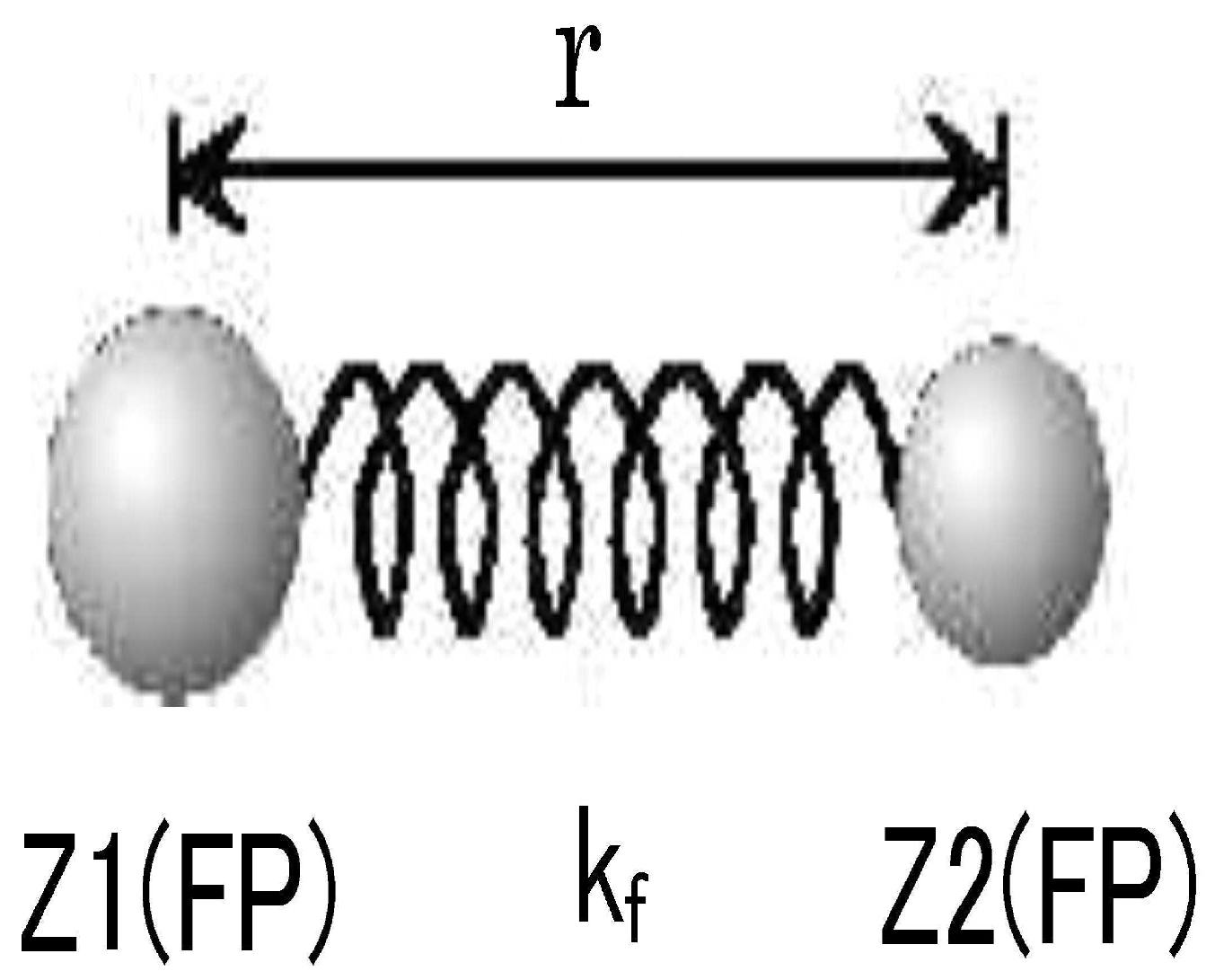
Figure 2. Relationship between nuclear fission process, potential energy, and effective fission distance

R_{e f f}

.

Figure 2. Relationship between nuclear fission process, potential energy, and effective fission distance

R_{e f f}

.

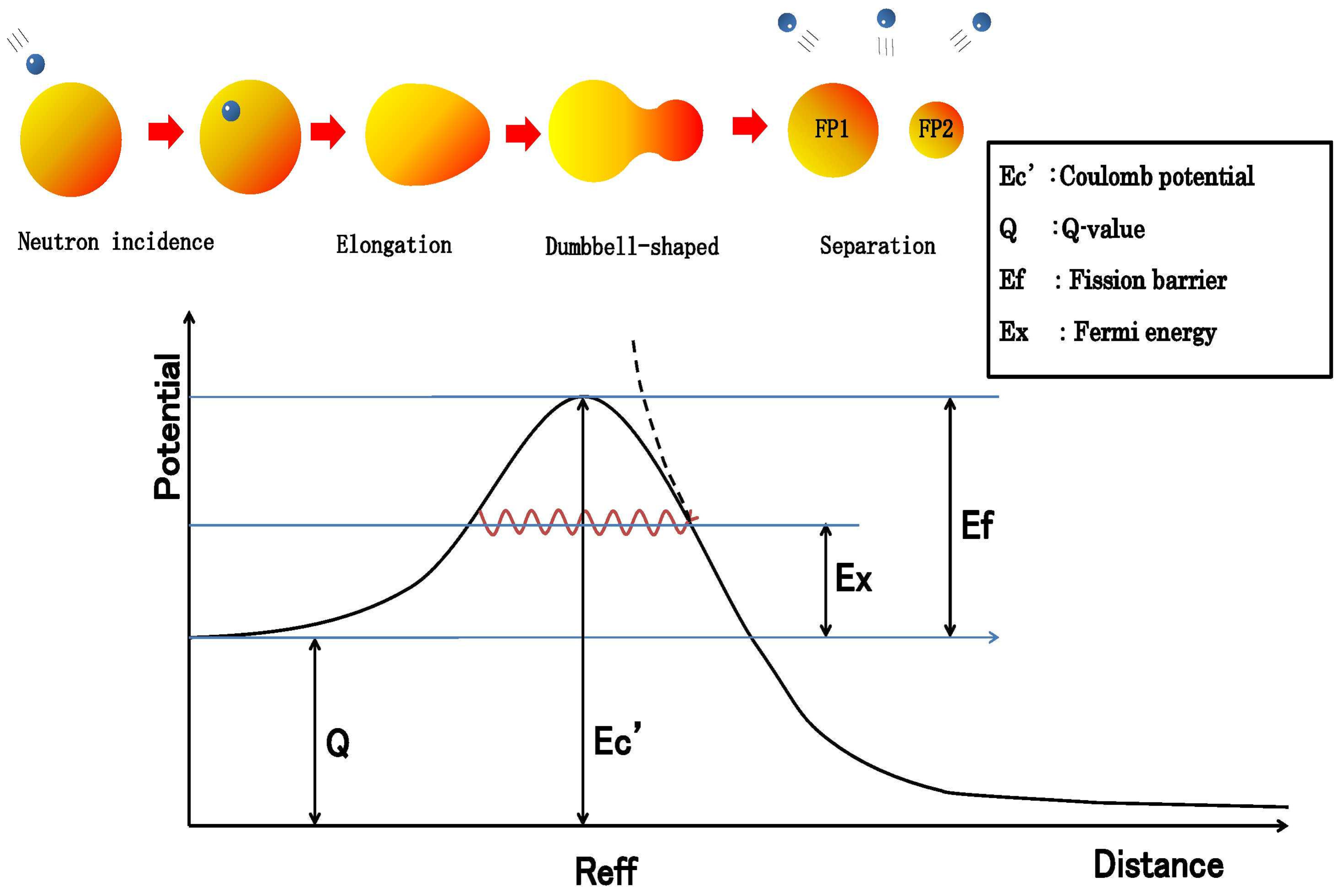
Figure 3. Relationship between atomic nuclear radius and potential energy.

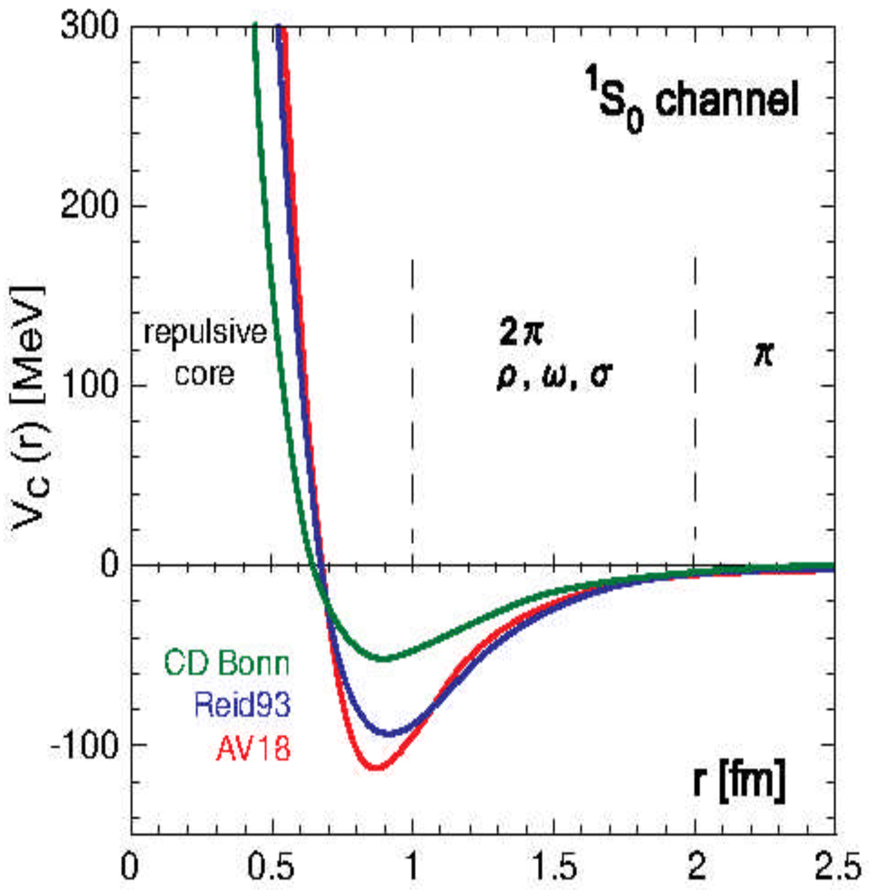
Figure 4. Charge number dependence of effective fission distance for

{}^{235}U

(incident neutron energy: 0.0253eV).

Figure 4. Charge number dependence of effective fission distance for

{}^{235}U

(incident neutron energy: 0.0253eV).

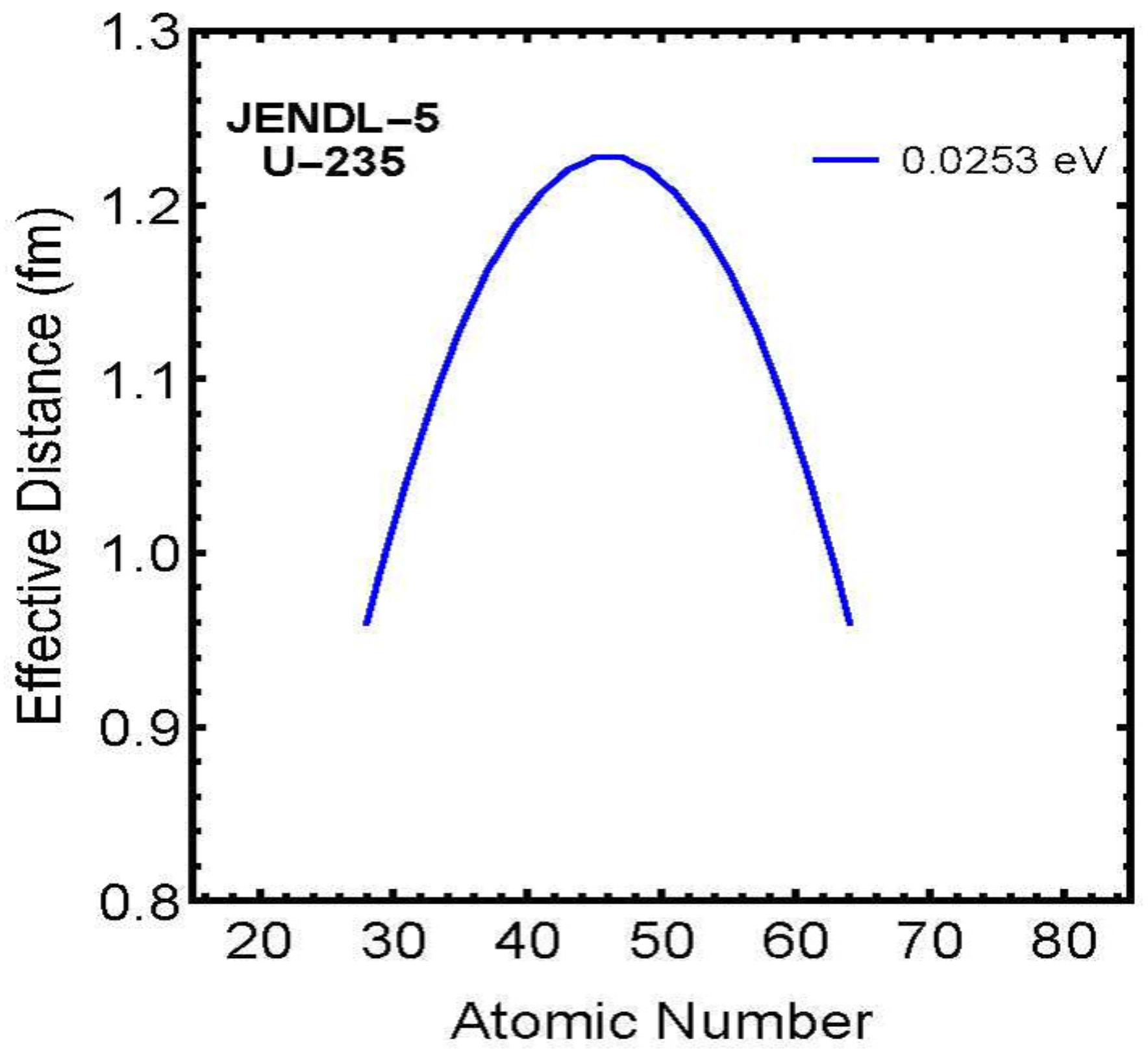
Figure 5. Charge distribution (theoretical curve) at zero Fermi energy (ground state) and experimental values for

{}^{235}U

.

Figure 5. Charge distribution (theoretical curve) at zero Fermi energy (ground state) and experimental values for

{}^{235}U

.

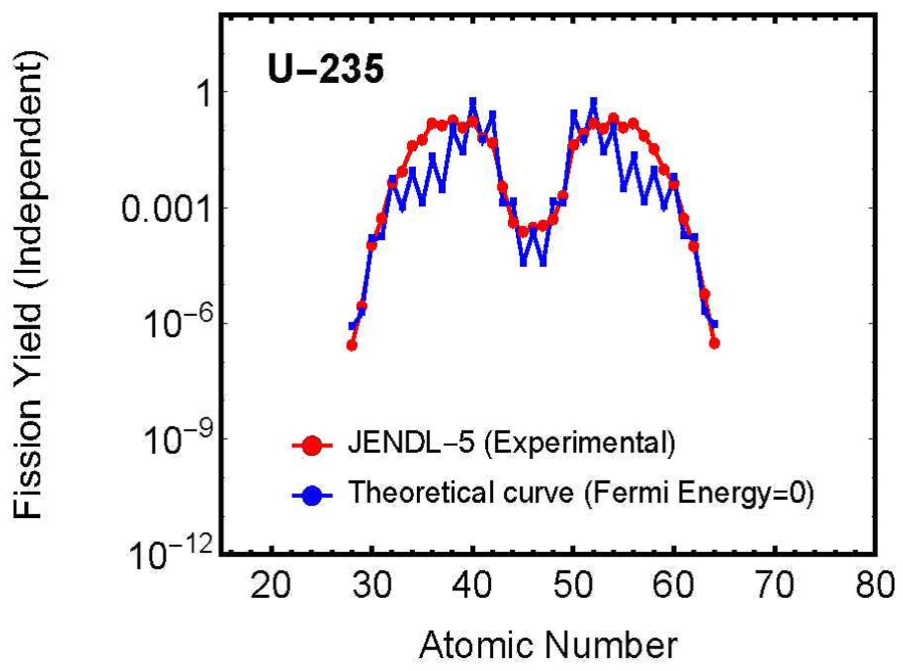
Figure 6. Relationship between Fermi energy distribution (blue line) and charge distribution (gray line) versus fission fragment charge number for

{}^{235}U

(incident neutron energy: 0.0253eV).

Figure 6. Relationship between Fermi energy distribution (blue line) and charge distribution (gray line) versus fission fragment charge number for

{}^{235}U

(incident neutron energy: 0.0253eV).

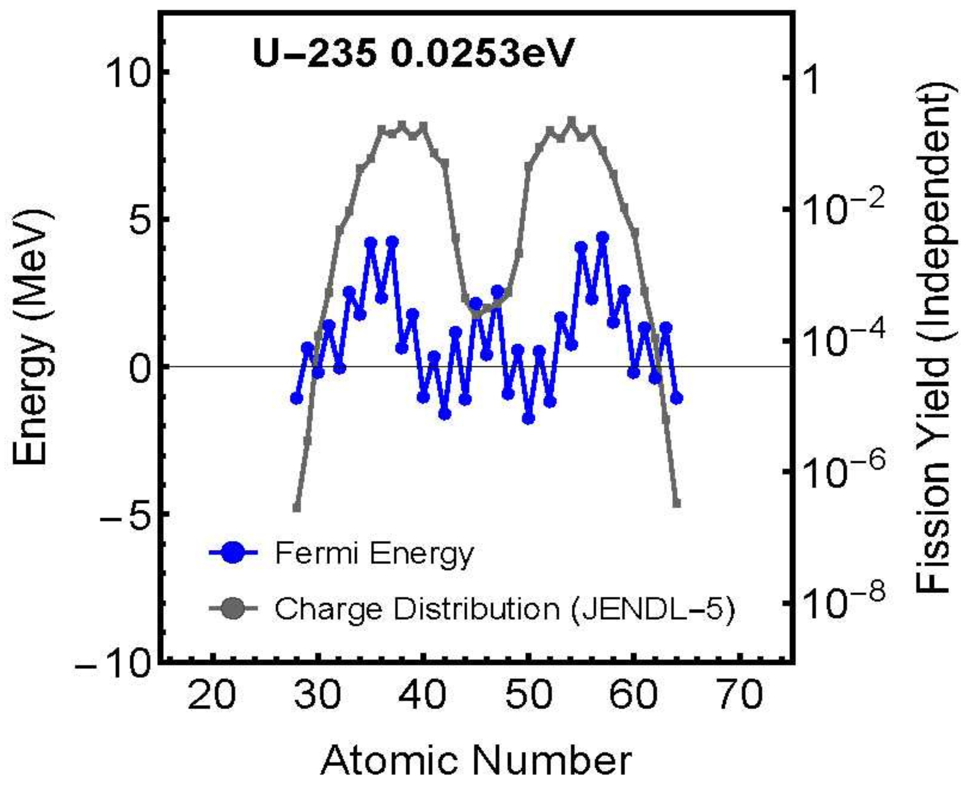
Figure 7. Conceptual diagram and emission spectrum of spontaneous emission light in semiconductors (excerpted from "Introduction to Optical Devices" by Professor Suemasu).

Figure 8. Energy spectrum of prompt neutrons (excerpted from Professor Abe’s website).

Table 2. Comparison of maximum Fermi energy values and fission barrier energies.

Nuclide	Maximum Fermi Energy (MeV)				Generally Predicted
	0.0253eV	500keV	14MeV	Average	Fission Barrier (MeV)
²³²Th	-	6.19	5.50	5.84	6.0∼6.3
²³³U	3.26	3.26	2.29	2.94	5.7∼6.0
²³⁵U	4.13	3.57	3.85	3.85	5.8∼6.0
²³⁸U	-	5.54	5.45	5.50	6.0∼6.2
²³⁷Np	3.43	3.16	2.29	2.96	5.8∼6.0
²³⁹Pu	4.72	4.25	4.12	4.36	5.9∼6.0
²⁴⁰Pu	5.36	4.84	4.51	4.90	5.8∼6.1
²⁴²Pu	6.48	5.98	6.69	6.38	6.0∼6.2
²⁴¹Am	4.72	4.25	4.12	4.36	5.9∼6.1

Disclaimer/Publisher’s Note: The statements, opinions and data contained in all publications are solely those of the individual author(s) and contributor(s) and not of MDPI and/or the editor(s). MDPI and/or the editor(s) disclaim responsibility for any injury to people or property resulting from any ideas, methods, instructions or products referred to in the content.

© 2024 by the authors. Licensee MDPI, Basel, Switzerland. This article is an open access article distributed under the terms and conditions of the Creative Commons Attribution (CC BY) license (http://creativecommons.org/licenses/by/4.0/).

Copyright: This open access article is published under a Creative Commons CC BY 4.0 license, which permit the free download, distribution, and reuse, provided that the author and preprint are cited in any reuse.

Application of the Hill-Wheeler Formula in Statistical Models of Nuclear Fission: A Statistical Mechanical Approach Based on Similarities with Semiconductor Physics

Abstract

Keywords:

Subject:

Introduction

Overview of Statistical Mechanical Nuclear Fission Model

Basic Framework of the Selective Channel Scission Model

Introduction of Statistical Mechanical Interpretation

Calculation Using the Hill-Wheeler Formula in Nuclear Fission Statistical Model

Calculation Conditions

Reasons for Considering the Hill-Wheeler Formula as Nuclear Fission’s Quantum Mechanical Distribution Function

Derivation of the Nuclear Fission Statistical Model

Calculation Process from Nuclear Fission Statistical Model to Charge Distribution

Specific Calculations

Results and Discussion

Physical Significance of Effective Fission Distance Between Fragments

Significance of Charge Distribution Reproduction in Ground State

Inhomogeneity of Fermi Energy Distribution

Fermi Energy and Fission Barrier

Neutron Spectrum ∝ Density of States × Fermi-Dirac Distribution Function

Spectrum of Spontaneous Emission Light in Semiconductors

Energy Spectrum of Prompt Neutrons

Conclusions and Future Prospects

Precise Determination of Neutron Emission Numbers for Each Fission Fragment

Multidimensional Analysis of Fermi Energy Distribution

Extension of Theoretical Model

Acknowledgments

Appendix A. Theoretical Approach in Deriving Fission Distance

Appendix A.1. Limitations of Simple Fitting Methods

Appendix A.1.1. Problem of Negative Distances

Appendix A.1.2. Simplification of Energy Dependence

Appendix A.1.3. Lack of Physical Constraints

Appendix A.2. Advantages of Our Hill-Wheeler Formula Based Approach

Appendix A.2.1. Guarantee of Physical Consistency

Appendix A.2.2. Inclusion of Quantum Mechanical Effects

Appendix A.2.3. Proper Consideration of Energy Dependence

Appendix A.3. Prospects for Theoretical Approach

Appendix B. Detailed Description of the Three Main Calculations

Appendix 1. Derivation of the Effective Nuclear Fission Distance R eff

Appendix B.3.3.1. Derivation Process

Appendix 2. Charge Distribution Calculation Assuming Zero Fermi Energy

Appendix B.3.3.2. Calculation Process

Appendix 3. Determination of the Fermi Energy Distribution for Each Fragment

Appendix B.3.3.3. Calculation Process

Appendix C. Attached MATHEMATICA Calculation Program

References

MDPI Initiatives

Important Links

Subscribe