Introduction
American ginseng
Panax quinquefolium is one of the medicinal crops in Liuba County, Shaanxi Province, China. However, diseases and insect pests infested the crop, resulting in significant damage [
1,
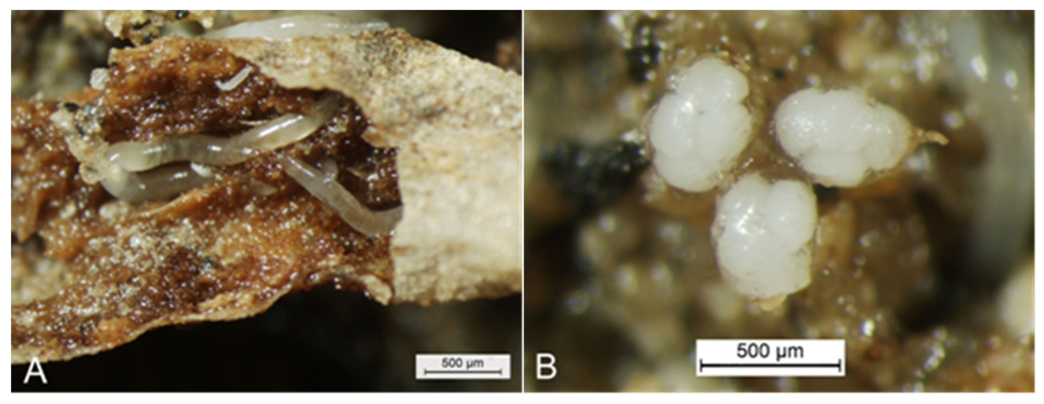
2]. In recent decades, some underground pests, including the worm
Enchytraeus buchholzi Vejdovský (Clitellata: Enchytraeidae) [
3,
4,
5] (
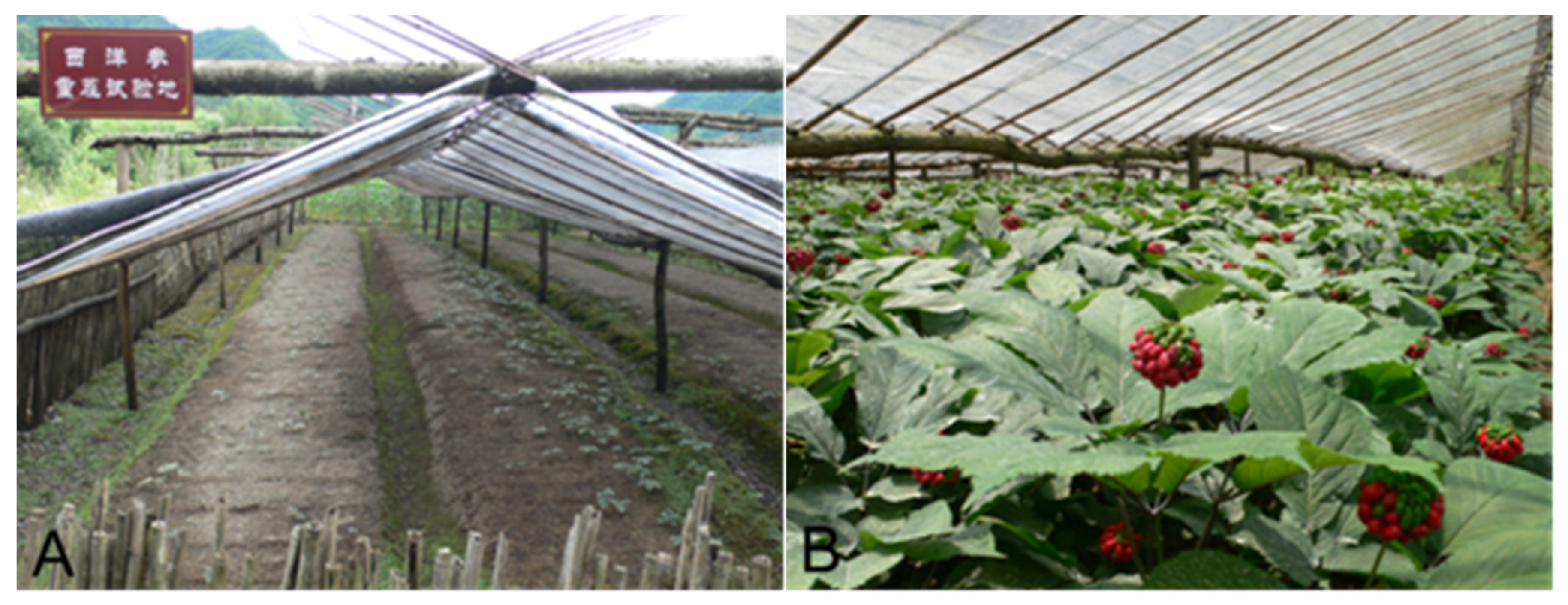
Figure 1), were discovered to attack the perennial, medicinal herb by roots, resulting in abnormal reduction of seedlings in nursery beds and severe losses of yields [
6] (
Figure 2).
Specimens of the worm collected from Liuba County were sent to an institute for scientific identification, but they were misidentified as
Enchytraeus bulbosus Nielsen & Christensen in 2014 [
7]. Although the scientific name was incorrect, our project team has studied the worm in following aspects: pesticide screen [
8], chemical control [
9], physiological time [
10], field temperature properties [
11], bionomics [
12], economic benefits and protective measures [
6], feeding amount and generational fertility [
13]. The worm was re-identified into
E. buchholzi in 2022, and thus recovered its original identity [
4].
Studying reproductive potential and population growth is an important work in animal ecology, and is usually conducted by testing and analyzing life tables of animals [
14]. As a monoecious species and about 5 mm long in adult stage, the worm feeds inside germinating seeds and roots of the host plant, and has a population with overlapping generations. When field conditions were imitated and the worm was reared in wet-sandy dishes in the laboratory, adults lived a very long life, laid many cocoons containing eggs in succession, and wrapped them with dusts [
13]. Individuals of the worm with different ages were present in smaller wet-sandy dishes and hid in food particles and sandy soils, which led to the situation that their number could not be accurately counted until the dishes were examined thoroughly by using a rinse method [
13]. But the rinse method was bound to change rearing conditions, which would stop the conventional life table method from being applied in present study. Therefore, the authors turned to measure individual fecundity of the worm in its lifetime, which led directly to a study of its individual reproduction. Meanwhile, the authors managed to estimate its laboratory population growth in another experiment through rearing the worm together with its offspring for a time longer than two generations.
Conventional theory in ecology holds up that an animal population follows exponential growth under favorable conditions first, and then logistic growth [
14]. Here, we tested if the population of
E. buchholzi follows the same growth trends, even within its individual reproduction process.
We then reflect on its reproductive behavior, by building statistical models, and linking numerical growth trends together with population growth.
Materials and Methods
Preparation for the Worm
Roots of American ginseng damaged by underground pests were collected from Liuba County, Shaanxi Province, China. Living specimens of E. buchholzi were picked out from the roots and placed into plastic dishes containing both wet fine sandy soils and American ginseng powders to isolate and rear populations at constant 21 °C. These populationsserved as our indoor stock colony for the following experiments.
Experimental Design and Execution
Applying a completely randomized design, the authors conducted two related experiments: 1) individual reproduction; and 2) population reproduction. After that, we analyzed the data with statistical and modeling methods.
Experiment I: Individual Reproduction – Measurement of Cocoons and Eggs Laid by a Parent Adult in Its Lifetime
Based on soil temperatures measured in the worm-infesting region in early August [
11] and per capita reproduction and daily mean reproduction of the worm indoors [
13], we selected 18 and 21 °C for the experimental treatments, and conducted the experiment by rearing worms at the two temperatures: 14 adults at 18 °C and 14 adults at 21 °C, that is, 14 replications for each treatment. We used a total of 28 adults as parent, and reared each of them alone in a 3.5 cm diameter, wet-sandy dish (see next paragraph for detail). Measurement of individual fecundity included: 1) the number of cocoons; 2) the number of eggs per cocoon; and 3) the number of eggs.
A batch of 28 polyethylene plastic dishes, 3.5 cm in inner diameter or 9.62 cm2 in inner area, was taken as rearing container. Both 4 g of sterilized fine sandy soils (passed through 60-mesh screen; aperture = 0.30 mm) and 1.2 mL of distilled water were added to each dish, which was vibrated to flatten the wet-sandy surface; extra water was sucked out, and then 10 mg of sterilized American ginseng powders (passed through 50-mesh screen; aperture = 0.36 mm) was dusted to the wet-sandy surface of each dish. They were called the “wet-sandy dish” or “dish” for short, and used in the rearing experiment.
A total of 28 subadults [
15,
16] (a subadult is here an individual of the species that has entered into its preoviposition stage, when one or two gray-white eggs are formed in its oviduct but have not been laid out yet.) were picked out from the indoor stock colony, and each of them was inoculated into a wet-sandy dish alone. After inoculation, the 28 dishes were randomly divided into two groups, with each group transferred into a thermostatic cabinet (Type 250D, Jintan Jerier Electrical Appliance Co., Ltd. China) at 18 °C or 21 °C respectively and reared. The RH was about 100% above the wet-sandy surface inside each dish. The two cabinets were placed in a shaded laboratory, with very weak sunlight diffused through the front glass window, and shifted naturally with day and night.
The worm inoculated into each dish was checked once every two days during the experimental or rearing time, when each dish was placed under a binocular stereo microscope, and the parent adult matured from initial subadult and its cocoon(s) laid inside the dish were found and recorded. A total of 98 records were obtained from each dish in the process. All the cocoons were removed or sampled from each dish when checked each time, and then combined to form a cocoon sample on that date [on the variable “eggs per cocoon (EPC)”, a t-test showed there was no significant difference (P > 0.05) between cocoon samples from both treatments on the same day, thus combined together]. In early stage of the microscopic examination, every cocoon in each sample was dissected immediately to record the number of eggs enveloped within; the frequency of dissection was changed to once every four days in middle and later stages; as a result, a total of 1,522 cocoons, or 52 cocoon samples combined, were dealt with in this way. After each checking, some sterilized American ginseng powders and water were added to each dish accordingly to maintain a proper living condition for the worm tested.
Experiment I was conducted under a semi-sterilized condition. In order to reduce food contamination caused by ambient miscellaneous microbes, a new batch of 28 wet-sandy dishes was prepared in the same way every 30 to 40 days, and the parent adults were then moved from the old dishes to the new ones to live and reproduce till their cocoon output extremely lowered. The experiment lasted for 196 days; the raw data before day 185 were adopted, but the rest were ignored because of many zeros.
Experiment II: Population Reproduction – Measurement of Laboratory Population Growth during a Time Longer than Two Generations.
Here, we set up different rearing time of adults as the experimental treatments, 8 in total, with each treatment repeated 7 times.
Another batch of 49 polyethylene plastic dishes was taken as rearing container. They were also prepared into wet-sandy dishes as shown in Experiment I; a subadult was inoculated into each of them and reared at 21 °C in a thermostatic cabinet. Each of the subadults matured alone and then reproduced together with its offspring in the same dish to form a laboratory population. The parent adult and its offspring in each dish were observed once every two days during the rearing time, and sufficient sterilized American ginseng powders and water were added to each dish accordingly to maintain an appropriate living condition, with the other conditions the same as those in Experiment I.
The 1
st sample was a visual one and obtained one day before an F
1 cocoon was laid, with its date code assigned as day 0. The day when the incidence of new cocoons reached 50% was monitored in the 49 wet-sandy dishes, labeled as the start of F
1 generation, and coded as day 1 in the following statistical analysis. With each sample containing seven wet-sandy dishes, the 2
nd one was drawn on day 3, and the 3
rd to 8
th ones were taken once every four days since day 11. Except the 1
st one, the rest samples were each taken randomly, and a thorough examination was performed immediately, that is, contents in each dish were rinsed three times with 10 mL of water. The rinse solution was collected in a watch glass, and examined under a binocular stereo microscope, with the sampling date and the number of adults, young worms and solid cocoons in each dish recorded. Experiment II ended after 35 days, in which the subadults took 4 days to mature and then reproduced for 31 days together with their offspring. The period of 31 days was 3 days longer than 2-generation time (GT, = length of immature and preoviposition stages) of the worm at the same temperature [
10].
Statistical Analyses
Experiment I: Individual Reproduction
Designation of Independent and Dependent Variables
Each sample date was coded in an ordinal manner starting day 0 as the day the subadults were inoculated, and the series of the codes was taken as an independent variable (T). The 0.5th, 2nd, 3rd, 4th and 5th powers of each code in the T variable (T1/2, T2, T3, T4 and T5) were calculated, constituted several different series (datasets), and taken as more independent variables (Ts).
Based on 14 replicates from each treatment on each sampling date, corresponding mean survival rate (SR) of the parent adults was calculated, and so were the 2-day mean cocoons (2DMC) on the same day. Two variables were then calculated along the ordinal date codes based on 2DMC, as follows:
Daily mean cocoons (DMC) = each 2DMC was divided by 2;
Cumulative cocoons (CC) = each 2DMC was added one after another till the end.
The mean number of eggs per cocoon (EPC) was calculated based on each cocoon sample on that day. EPC itself formed a variable, and was used to calculate the other two variables:
Daily mean eggs (DME) = each EPC was multiplied by the DMC on the same day;
Cumulative eggs (CE) = each EPC was multiplied by the 2DMC on the same day to form each 2-day mean eggs (2DME), and the latter was added one after another till the end.
Except for SR, variables DMC, CC, EPC, DME and CE were each taken as a dependent variable (Y), respectively.
Simulation of Relations Between CC or CE and T by Applying Exponential and Logistic Functions
Variables
CC and
CE were log-transformed accordingly. Via the least square method, linearized exponential and logistic equations were built through a correlation and regression analysis between the log-transformed values of
CC or
CE and
T itself, and these linearized equations were then transformed back to real ones [
14,
17,
18]. Meanwhile, against both the linearized and the real equations, the residuals between the observed and the fitted values (for the linearized equations, those between the transformed points and their estimates) were analyzed by using a chi-square goodness-of-fit test to find the probability if each of the newly built equations fit the observed (or transformed) points [
19,
20].
Stepwise Regression Analysis and Residual Analysis for Aptness of the Polynomial Regression Models Newly-Built
Via the matrix methods, each series of Y was regressed respectively on all the Ts in the backward stepwise regression procedure to build a polynomial regression equation. In each step, one of the Ts with the largest P-value (= with the smallest regression effect) was identified and eliminated on the basis whether the F-test ratio for its partial regression coefficient was significant at P ≤ 0.01 [
20]. After a linear (first-order), a quadratic (second-order), or a cubic (third-order) equation was constructed, a similar residual analysis was performed as described above [
19,
20]. Then, a derivative equation against each quadratic equation of CC or each cubic equation of CE was calculated, and the biological significances of the resultant intercepts (for the 1
st term) and slops (for the 2
nd and/or the 3
rd term) were specified and explained.
Both advantage and disadvantage of the exponential, the logistic, the quadratic and the cubic equations for
CC and
CE were compared and determined according to the higher aptness given by the chi-square goodness-of-fit test via residual analysis [
20]. Figures illustrating the trends of points and theoretical curves were plotted against
T, in order to compare effects fitted by each of the functions.
Division of the Filial Egg Stage into Many Substages, and Conversion of the Worms in Each Substage into Generational Adult Equivalents (GAE)
Based on the GT of the worm (
m ±
SD), 18.3 ± 0.47 days at 18 °C and 14.0 ± 0.50 days at 21 °C [
10], the filial egg stage ranging from days 3 to 185 was divided into 10 (at 18 °C) or 13 (at 21 °C) substages, with each substage equaling to a life cycle and containing a portion of
CE, or generational cumulative eggs (
GCE). Taken as in a closed population without concerning mortality, immigration and emigration, each 2
DME in the
GCE was converted into adult equivalents [
21] (AE, = subadults capable of reproducing soon) via being multiplied by development rate of the eggs in the substage, and summed to generational adult equivalents (
GAE), which was then divided by the
GCE to return an average development rate (
ADR). The formula to calculate
GAE was:
where,
Ei = the number of eggs laid on the
ith day in the substage,
Di = duration of the eggs from the
ith day to
m, and
m = the GT in days at the temperature.
Experiment II: Population Reproduction
Designation of Variables and Their Correlation and Regression Analysis
The codes of the eight sampling dates, including days 0 to 31, were taken as the independent variable
T, and the eight means of AE from corresponding samples as the dependent variable
Y. Both exponential and logistic functions were applied as usual respectively, and a linearized correlation and regression analysis of the transformed
Y on
T was conducted via the least square method; after back-transformation, two real equations for the laboratory population growth were built. In the meantime, a chi-square goodness-of-fit test was applied to the two real equations [
14,
17,
18,
19,
20]; when a higher fit probability was taken as the criterion, the proper regression model was determined, and the trend of AE varying with sampling date codes was plotted.
The two experiments were conducted in Shaanxi University of Technology, China, in 2015; their statistical analyses and theoretical study were performed intermittently and completed in 2024.
Results
Experiment I: Individual Reproduction
Survivorship of the Parent Adults
Throughout the rearing time, SR of the parent adults was maintained in a higher level. At 18 °C, SR was 100% through day 19, decreased gradually to 64.3% on day 185. At 21 °C, SR was 100% through day 49, and then lowered gradually to 71.4% on day 185.
Exponential and Logistic Equations for CC and CE with Their Aptness
When simulated with an exponential or a logistic function, in the phase of linearized analysis, the correlation coefficients (
r) of the log-transformed
CC and
CE (or
CC' and
CE' in
Table 1) on
T were all significant (
P < 0.001) (
Table 1).
χ2 values of the linearized regression equations ranged from 5.48 to 37.1, indicating their fit probabilities were close to 1.000 (
Table 1). After the linearized regression equations were transformed back, the
χ2 values of the resultant real equations increased sharply, ranging from 426 to 4,469, meaning their fit probabilities were very close to 0, except those of the two real logistic equations for
CC (
χ2 = 71.0 and
P ≈ 0.940 at 18 °C;
χ2 = 98.5 and
P ≈ 0.279 at 21 °C) (
Table 1). For the resultant real equations, these linearized correlation coefficients were no longer valid.
Polynomial Regression Models of Each Y on Ts
Stepwise regression analyses indicated that each of the five dependent variables,
DMC,
CC,
EPC,
DME and
CE, was closely correlated to
T and/or
T1/2,
T2,
T3 retained, with its linear or compound correlation coefficient,
r or
R, significant at
P < 0.001 (
Table 2). The
F-test ratios for partial regression coefficients of
Ts retained in the linear, quadratic, or cubic equation were all significant at
P < 0.001 (
Table 2), meaning their regression effects were all strong. The chi-square goodness-of-fit test indicated each of the
χ2 values was very low, meaning the probability that the estimates fit the observed points was larger than 0.9994; therefore the null hypothesis
H0 was concluded that the regression models fit the linear, quadratic and cubic growth trends (
Table 2).
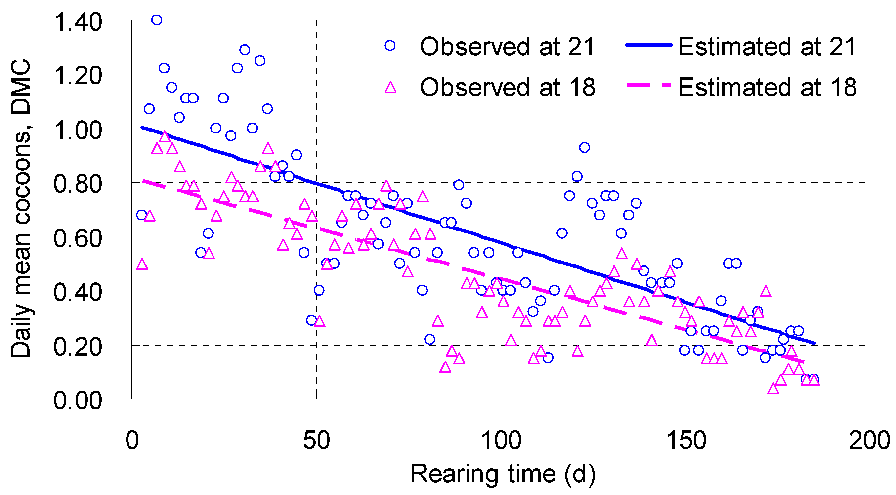
The number of
DMC increased rapidly with
T, reached its maximum between 7 and 9 days, and then fluctuated and decreased slowly, whose trend was fitted with a linear function (
Table 2;
Figure 3). The intercepts of the two linear equations were positive, with 0.816 cocoon a day at 18 °C and 1.02 at 21 °C; the slopes were negative, ranging from -0.00374 to -0.00439, meaning their regression lines were trending downwards (
Table 2;
Figure 3). The regression line associated with 21 °C located in the upper position, over the line with 18 °C, indicating that in the range tested the higher temperature was helpful for more cocoon output (
Figure 3).
Points were found fluctuating around the regression lines in
Figure 3, largely due to move of the parent adults into totally new wet-sandy dishes every 30 to 40 days, which caused valleys and recoveries of
DMC, appearing as several subcycles. They did add some noises but not affect the overall falling trends of
DMC. Similar phenomenon could also be perceived in other figures below.
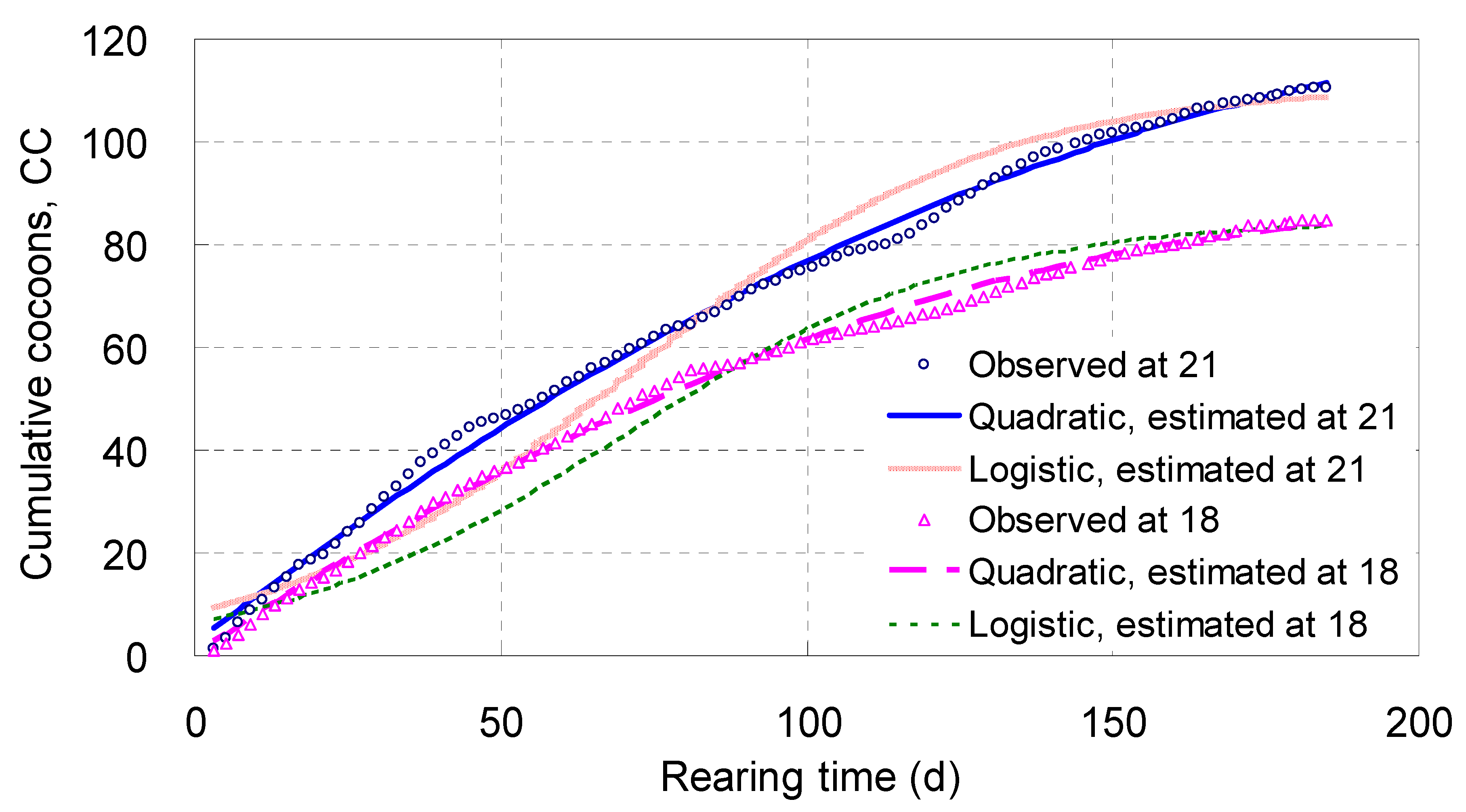
Cumulative Cocoons, CC
Cocoons appeared from zero to a certain number, and rose day by day;
CC increased steadily with
T along a quadratic curve, with its midrange arched, reflecting the pattern for cocoon growth (
Table 2;
Figure 4). Living at 18 °C for 185 days, each parent adult laid 84.8 cocoons on average; however at 21 °C the mean number was 110.6 (
Figure 4).
The
χ2 values of the
CC quadratic models were only 4.82 and 10.7, meaning their fit probabilities approached 1.0000 (
Table 2); whereas the fit probabilities of the real logistic equations of
CC were 0.940 at 18 °C and 0.279 at 21 °C (
Table 1). This comparison showed the simulating effects of the
CC quadratic models were better than those of the real logistic equations of
CC.
Figure 4 illustrated the tracks of the real logistic equations of
CC were systematically deviated from the observed points, much inferior to those of the
CC quadratic models. The real exponential curve was not drawn because of its extremely significant deviation from the observed points (
Table 1).
The derivative of each quadratic model for
CC on
T and
T2 was a linear equation (
Table 2), expressing the average efficiency of the parent adults' laying cocoons. When broken down, the intercepts expressed the coefficient of daily reproductive potential, which was 0.801 cocoon a day at 18 °C and 0.923 at 21 °C on average (
Table 2); their slopes represented the coefficient of reproductive resistance, which was -0.00377 and -0.00361, small but significant at
P < 0.001 (
Table 2).
Eggs per Cocoon, EPC
Independent variables retained in the
EPC cubic equation were
T1/2,
T,
T2 and
T3, and the
F-test ratios for the partial regression coefficients were all significant (
P < 0.001). The partial regression coefficient quantifying the variable
T1/2 (
b1 = 6.77) and its partial
F-test ratio (
Fb1 = 30.6,
P < 0.001) were each the largest, indicating this variable played the strongest role in constructing the
EPC model (
Table 2). In terms of absolute value, those partial regression coefficients quantifying
T,
T2 and
T3 became smaller orderly, and so did their partial
F-test ratios, meaning their roles lowered in the same way (
Table 2).
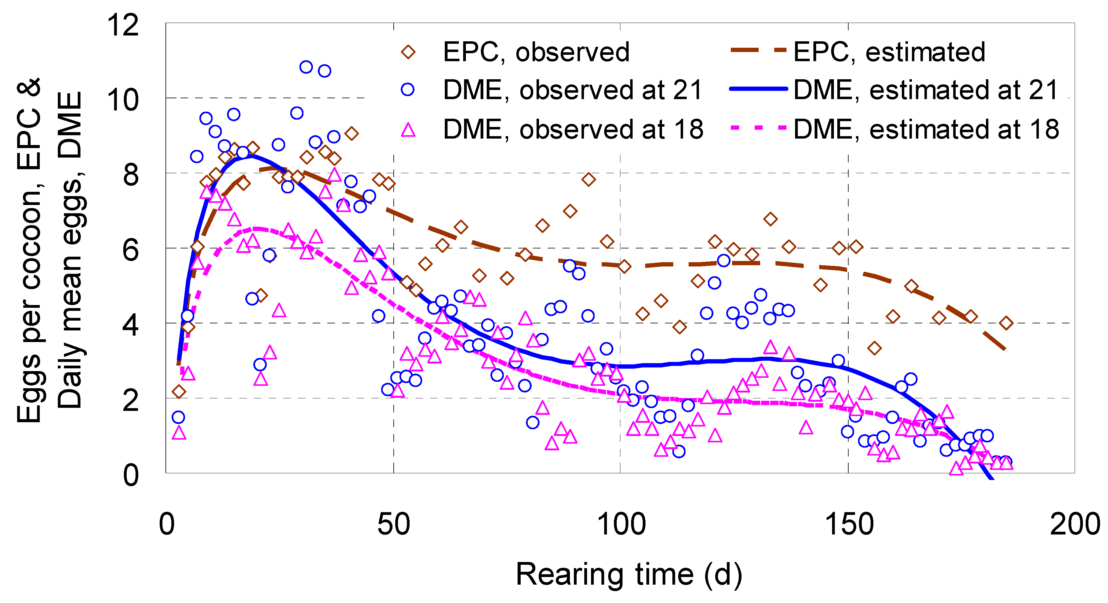
Figure 5 illustrated that
EPC varied with
T1/2,
T,
T2 and
T3 along a cubic curve. The estimate of
EPC was 2.9 eggs on day 3 of the rearing time, increased to the peak 8.1 on day 24, decreased gradually to 5.6 on day 90, nearly leveled off to 5.4 on day 150, and then lowered slowly to 3.3 on day 185. The daily mean of
EPC was apparently in constant change as the rearing time extended.
Daily Mean Eggs, DME
Independent variables retained in the
DME cubic equations were also
T1/2,
T,
T2 and
T3, and the
F-test ratios of their partial regression coefficients were all significant (
P < 0.001), too. They played almost the same role as their building the
EPC model (
Table 2).
The tracks of the
DME cubic curves ascended sharply in their initial stage, reached peaks around day 20, descended gradually for about 70 days, leveled off for about 60 days, went down again and terminated almost on day 185 (
Figure 5). At 18 °C, the estimates on days 20, 70, 90, 150 and 185 were 6.5, 3.1, 2.3, 1.7 and 0.1 eggs; while at 21 °C the estimates were 8.4, 3.7, 2.9, 2.8 and 0 eggs (
Figure 5). Trends of
DME illustrated that about 60% of the filial eggs were laid (though by means of cocoons indirectly, the same below) in the first 70 days, which was as long as nearly 4- or 5-folds of a GT of the worm at the temperatures tested [
10] (
Figure 5).
Cumulative Eggs, CE
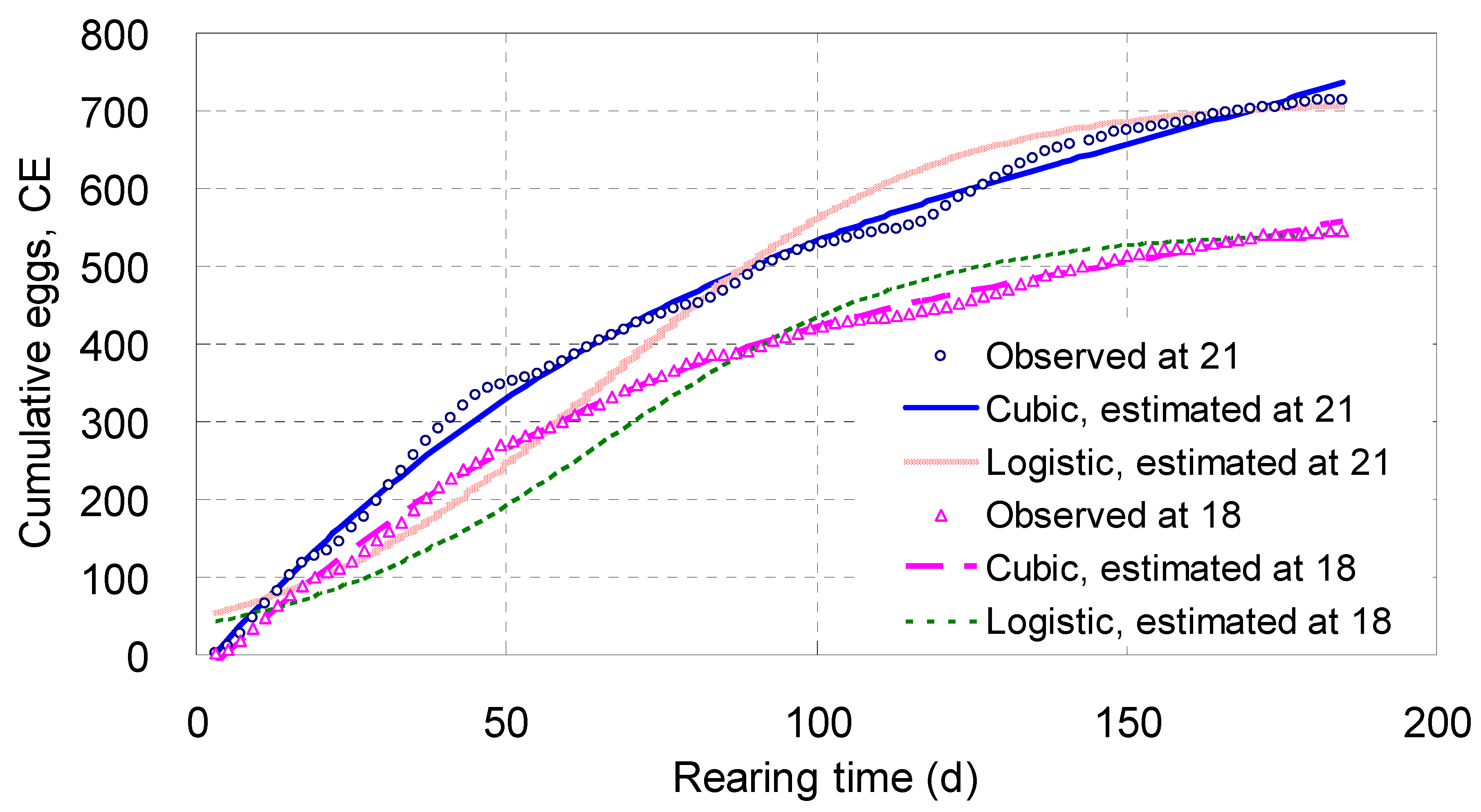
Shown in
Table 2 and
Figure 6,
CE increased steadily with
T,
T2 and
T3 along a cubic curve, and the arch in the midrange of each curve was more strengthened. Living at 18 °C for 185 days, each parent adult laid 545 eggs on average; and at 21 °C the mean number was 714 (
Figure 6).
The
χ2 values of the
CE cubic models were 34.9 and 48.8, meaning their fit probabilities were higher than 0.9999 (
Table 2); whereas the fit probabilities of both the real exponential and real logistic equations for
CE were close to 0 (
Table 1). These comparisons meant the simulating effects of the
CE cubic models were much better than those of the real exponential and real logistic equations for
CE.
Figure 6 illustrated the tracks of the real logistic equations for
CE were systematically and badly deviated from the observed points, and had therefore to be discarded. The tracks of the real exponential equations (not shown) were completely departed from the observed points and thus discarded, too. As a result, only the
CE cubic models were preferred here.
The derivative equation of each cubic model for
CE on
T,
T2 and
T3 was a quadratic one (
Table 2), expressing the average efficiency of the parent adults' laying eggs though the latter were enveloped in cocoons. When both derivative equations were broken down, the intercepts expressed the daily reproductive potential for a parent adult to lay eggs, which were 7.83 at 18 °C and 9.08 at 21 °C on average (
Table 2); the coefficients for the 2
nd term
T represented the reproductive resistance, ranging from -0.084 to -0.090 (
Table 2); those for the 3
rd term
T2 were minute positives (0.000274 and 0.000293), apparently a little compensation to the daily reproductive potential, increasing with the square of ordinal day.
Values of GCE, GAE and ADR as Well as Recognition of R0
Listed in
Table 3, the values of
GCE changed in different substages; numbers of
GAE that appeared in the first three sub-stages were 42.5, 41.3 and 48.5 AE (with an average of 44.1 AE) at 18 °C, and 41.2, 43.5 and 66.0 AE (with an average of 50.2 AE) at 21 °C, much more than those in other substages. Around means of 0.52,
ADR varied from 0.41 to 0.62 at 18 °C, and from 0.40 to 0.60 at 21 °C, owing to uneven numbers of partial
CE in each substage (
Table 3).
Now that
GAE was given in a GT or a life cycle, the value 42.5 AE derived from the first substage could be recognized as the net reproductive rate
R0 (or the net rate of increase per generation [
14]) of the worm at 18 °C; and in parallel the value 41.2 AE as
R0 at 21 °C. When the average of
GAE from the first three sub-stages was chosen as an alternative, the mean values 44.1 and 50.2 AE could also be determined as
R0 at 18 and 21 °C respectively. The rest values of
GAE would be underestimates of
R0 if they were used to do so (
Table 3).
Experiment II: Population Reproduction
When fitted in an exponential function,
Y (= AE representing the laboratory population densities) was closely and positively correlated to
T (
P < 0.001) after the dependent variable was transformed into its common logarithm (
Table 4). The linearized regression equation played only an intermediate or transitive role (acted as a bridge) though the low
χ2 value meant its fit probability was high (
P > 0.9998). However, when the linearized equation was transformed back to a real exponential one, the
χ2 value became very large, proving that its aptness was close to 0 (
Table 4), which was not accorded with the reality and should be discarded.
When fitted in a logistic function,
Y was closely and negatively correlated to
T (
P < 0.001) after the dependent variable was transformed according to its special rule (
Table 4). The
χ2 value of the linearized equation was low, meaning its fit probability was very high (
P ≈ 1.0000). When the linearized equation was transformed back to a real logistic one, the
χ2 value was 6.519, indicating that its fit probability approached 0.4806 (
Table 4), much larger than 0.05, worthy of adoption (
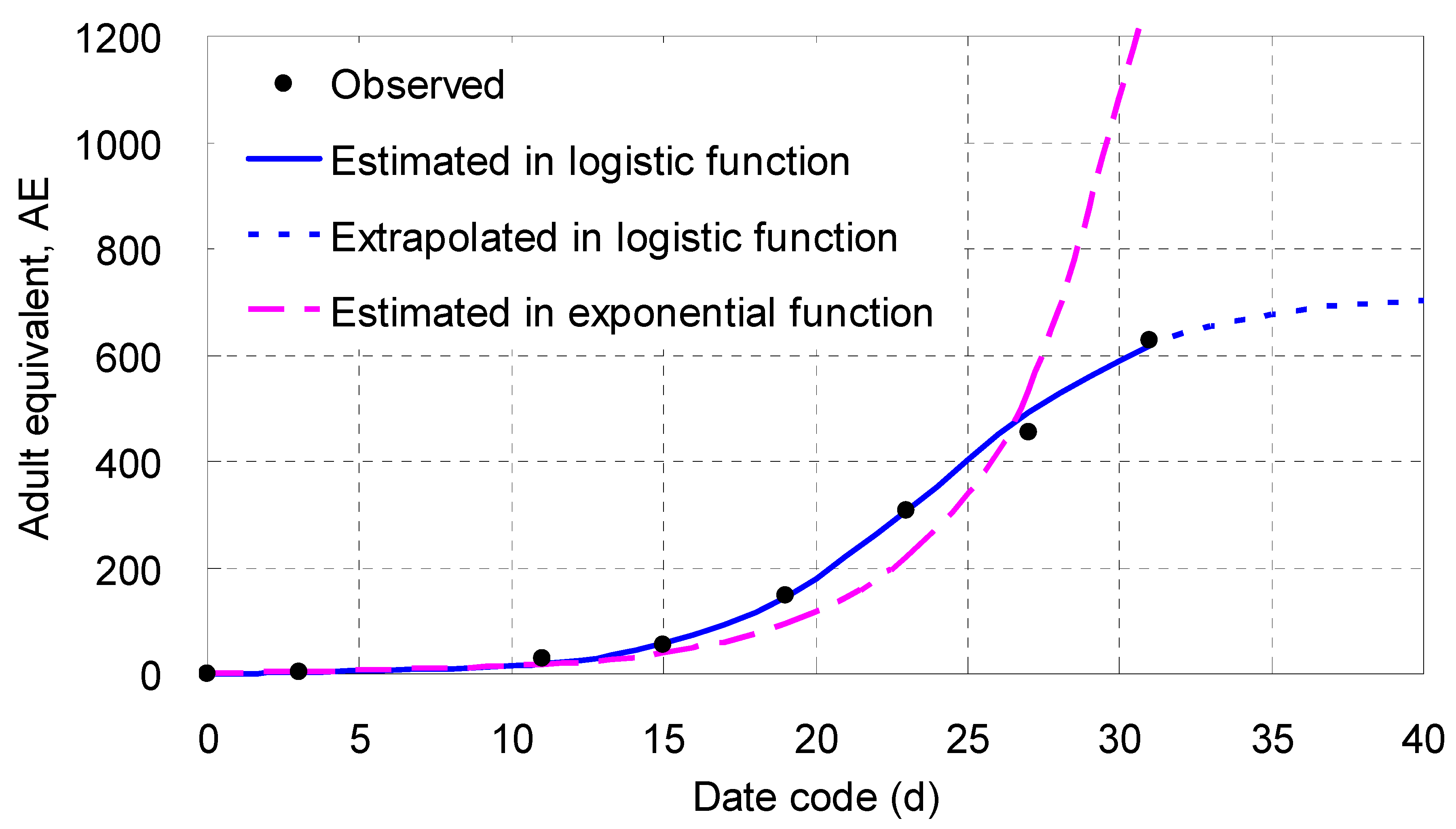
Table 4;
Figure 7).
Figure 7 illustrated that both the logistic and the exponential curves were close to each other on days 1 – 7 (the latter was the midpoint of the 1
st GT); afterwards, the logistic curve extended along the trend of the points observed, rose gradually and then leveled off slowly; whereas the exponential curve was biased from the rest points: declined first, went lower and lower, turned back on day 23, rose up rapidly, and then badly deviated on day 31. The two curves crossed on day 26.4, near the end of the 2
nd GT, when the instantaneous population density was up to 471 AE/9.62 cm
2, or 49 AE/cm
2, acting as if a critical value. The difference between the two curves became larger and larger since then.
Discussion
In Experiment I, the first part of present study, the authors started with measuring fecundity of E. buchholzi in its lifetime. Either observed or theoretical fitted, the shapes of the fecundity curves reflected general trends of individual reproduction of the worm. Because the worm lays eggs indirectly (it lays cocoons containing eggs), we conducted the measurement in three steps, which determined specific procedure and content of Experiment I, distinct from those of Experiment II that started with a population reproduction directly. It was worthwhile conducting both reproductive experiments indoors so as to find evidence to predict population growth trends in the field.
Polynomial Growth Trends in Individual Reproduction
As shown in Experiment I, higher survival rate, much longer life span, and larger daily reproductive potential of the parent adults were detected. Compared with the GT in broad sense, the filial egg stage ranging from days 3 to 185 was as long as a period of time for 10 or 13 full generations to take place at 18 or 21 °C, which proved that E. buchholzi belonged to a type of long-living species.
The derivative equations for the CC quadratic curves allocated coefficients for daily reproductive potential and resistance. Expressed by each intercept, the daily potential was the inherent power for parent adults to reproduce; while the resistance, represented by each slope, was their response to increase of ages because instant number or density of the worm in a dish was extremely low, or in other word, density-independent.
Although the intercepts and slops given by the CC derivative equations were slightly different from those of the DMC linear models, the former provided an adequate support to the latter; both achieved a mutual verification, showing that the daily reproductive potential interacted with the resistance each other, thus formed the actual number, the daily reproductive capacity, of DMC on each day. Compared with the CC quadratic models, the CC logistic equations showed a much lower aptness to points observed, thus ought to be discarded.
Suitable simulations to the varying trends of EPC and DME were attained by applying cubic equations, including the square root of T as one of the independent variables. Both types of cubic curves reflected trends how the number of eggs changed with rearing time.
Based on continuous changes of EPC and DME, two CE cubic equations were built at 18 and 21 °C, which realized a sufficient simulation to actual facts. The derivative equations for the CE cubic models also differentiated the egg growth trend into coefficients of daily reproductive potential and resistance, and even added a tiny supplementary coefficient to the former. Whereas indicated by the huge χ2 values, the real exponential and real logistic equations for CE exhibited extremely small aptness, showing they lost contact with reality and had to be abandoned.
The common trends of the increment curves resulted from the DMC, EPC and DME equations were that points appeared initially in a low position, rose rapidly, fell down slowly, and vanished eventually, and those of integral curves from the CC and CE equations were that their values increased more quickly in early range than those in later one, and leveled off finally. The higher increments or more-convex ranges in early stage were induced by vigorous reproductive capacity, whereas the lower increments or less-convex ranges in later stage were caused by senescence of the parent adults. Just as shown above, resulted from individual reproduction, these trends could be described only by polynomial regression models but neither by exponential nor by logistic equation. Under this situation, as a portion of the whole reproductive process, the population in the first GT should have taken on a polynomial growth rather than others, even though it consisted of only filial eggs that would develop into adults in the future.
Basis and Application of R0
Both eggs and young worms cannot be compared with adults in that their instantaneous reproductive capacities are zeros, totally different from the latter, even though the former may grow up to the latter after completing a generational development. However, based on their development rates in a life cycle, a conversion of eggs and young worms into AE made this comparison possible [
13]. Following the same rule, both a reasonable division of the filial egg stage into many substages, with each equaling to a GT, and a conversion of eggs in each substage into
GAE were performed. Measured in the quantity of subadult,
GAE represented a group of offspring reproduced by a parent adult in a GT, which was convenient to compare with results of previous study on the one hand, and revealed the important term
R0 on the other hand.
Living together with offspring in a smaller wet-sandy dish (1.5 cm in inner diameter) for a life cycle, the worm showed its actual generational fertility [
13] (with the same meaning as current variable
GAE). The values of
GAE derived from the first substage of Experiment I (42.5 AE at 18 °C and 41.2 AE at 21 °C, as indicated above) were close to them, and therefore got verified by an example from population reproduction outside. Furthermore, estimated from the real logistic equation built in Experiment II, the laboratory population density was 43.5 AE (including 1 parent adult) in a wet-sandy dish by the end of the 1
st GT (day 14), approaching the
R0 just obtained from Experiment I. Conducted under different rearing and sampling schemes, the three experiments had given estimates that were statistically similar to the value of
R0.
In broad sense,
R0 is applied to estimate population growth of living things, and calculate economic threshold as well [
22]. Exponential growth of a population is described by the formula,
Nt =
N0ert [
14], in which the power
er may be substituted by the term
R0; if so, the formula became
Nt =
N0R0t, an equivalent expression. If the following numbers were referred, for example,
N0 = 1 (the initial number of parent adult),
R0 = 41.2 (the number of AE by the end of the 1
st GT), and
t = 2 (the number of GT), the equivalent formula could estimate
N2 = 1 × 41.2
2 = 1,697, meaning that the population size of the worm would reach 1,697 AE by the end of the 2
nd GT (day 28) if the ambient resources, especially the rearing area, were unlimited.
Logistic Growth Trends in Population Reproduction
As shown in Experiment II, especially illustrated in
Figure 7, the laboratory population density did not follow exponential but logistic growth when the worm was reared in the wet-sandy dish for a period of time longer than two generations. Compared in terms of AE by the end of the 2
nd GT, the estimate given by the real logistic equation from Experiment II was only 533 AE, much lower than the estimate (1,697 AE) from the hypothetical example given above. The difference between the two estimates was huge indeed, and the strong descending effect demonstrated the laboratory population was density-dependent. This enormous inhibition was actually caused by over-crowding of more offspring born within the limited area inside the wet-sandy dish. Referring to the information reflected in Experiment II, we may deduce that the longer is the duration when the worm is reared in a limited area, the stronger is the inhibition that depresses its population density in the same site.
There arises a question herein: when to apply an exponential function and when a logistic one? According to the experimental study, the suggestion might be applying an exponential function to simulate and describe a population size when it lives in an ecological niche with ambient resources unlimited, or “under favorable conditions” [
14]; otherwise, it may be the first choice applying a logistic one to simulate and estimate a population density if the ambient resources are limited and corresponding model is verified through, just as the example from Experiment II, in which one of the resources, the rearing area, was limited. Resources are often limited in the biosphere, and thus, exponential growth is perhaps not as common as logistic growth in the field of population ecology if the period of observation is longer enough, lasting for 2, 3 or more GT.
More Considerations
By the experimental study, we have found two kinds reproductive potentials, daily and generational; the former is expressed by intercepts of the derivative equations of polynomial growth models for cumulative cocoons and eggs, and the latter is indicated by adult equivalents generated by a parent worm in a full generation time, equaling to R0. Each has its own applying values.
An actual population possesses two attributes in an ecological niche: temporal and spatial, meaning that it exists and develops in a definite time and space. The laboratory population of
E. buchholzi generated by population reproduction in Experiment II was such an actual one. Whereas, the laboratory population of
E. buchholzi generated by individual reproduction in Experiment I had only temporal attribute; its spatial attribute was extremely weakened by artificially removing of the cocoons on each checking day, leaving only a parent adult laying cocoon(s) lonely in a dish. It was never a hypothetical population as cocoon(s) appeared continuously. Once its spatial attribute were supplemented fully in its ecological niche, this kind of temporal population would put its generational reproductive potential into effect rapidly, leading to actually huge populations to feed on their host plant American ginseng! Theoretically, the worm reproduces 7 to 9 generations a year [
11], about 42 AE a generation, and an AE eats away 1.19 mg of fresh ginseng (excluding more tissues contaminated) [
13]. What a devastating economic loss would that cause?!
Modeling is one of the special research methods, and needs to be verified by other theory and/or practice; theoretically, statistical tests can be effective to some extent. It should be admitted that the chi-square goodness-of-fit test included in the residual analysis [
20] is important, which identifies if the fitted regression model is justifiable, especially when data transformation and a back-transformed equation are involved, where the correlation coefficient can only be meaningful to the linearized form, but invalid for the back-transformed equation reflecting the real relationship, as shown in present study. Only are well-constructed real equations or models able to make correct predictions and help solving practical problems.
It will be helpful to solve and explain some similar research problems if the methods used in the experimental study are applied to relevant fields.
Conclusions
On the basis of results and discussions just stated above, the authors concluded that:
1) The DMC linear equations and the CC quadratic equations were succeeded in fitting the trends of cocoon growth; the former described daily changes of cocoons, and the latter expressed their accumulated effects.
2) The EPC cubic equation properly simulated changes of egg numbers in cocoons, so that subsequent calculations and analyses would be continued.
3) The cubic equations of DME and CE were succeeded in fitting the trends of filial egg growth; the former displayed daily increments of eggs, and the latter reflected reproductive outcomes of individual parent adults.
4) Polynomial regression equations as such were shown to be suitable models for individual reproduction of the worm E. buchholzi at 18 and 21 °C, whose daily reproductive potential and resistance were quantified by the derivative equations, and both interacted and formed its reproductive capacity, meaning a quantitative expression of its reproductive behavior.
5) GAE was calculated via a conversion of filial eggs into AE, and the GAE from the first substage functioned as R0 of the worm. As a living material base accumulated by individual reproduction in F1 generation, and taking t (the number of generations) as its index, the R0 would play an essential role in exponential growth of E. buchholzi population size since F2 generation if resources were unlimited.
6) Living together with its offspring in a limited area, the laboratory population of the worm bypassed an exponential and directly followed a logistic growth from F1 to F3 generations.
7) The hypothesis of exponential growth was disproved by population reproduction of E. buchholzi living in a limited area; neither exponential nor logistic growth was seen appearing in the process and result of individual reproduction of E. buchholzi, showing the conventional theory was not applicable in this aspect. And
8) Revealing these statistical relationships helps professionals comprehend individual reproduction of E. buchholzi clearly, understand the logical sequence and the difference between individual and population reproductions better, predict its population dynamics properly, develop its IPM program, and promote a stable and high productivity of American ginseng. The experimental study has expanded theories on bionomics and population ecology of E. buchholzi, and opened a new area for research work in related fields.
Author Contributions
LMZ conceived and designed the experimental study, analyzed, modeled and interpreted the data, and wrote and revised the manuscript. GLM participated in the experiments, collected and collated most data, and drafted part of contents. All the authors read and approved the final manuscript.
Funding
The study was part of the project “Studies of the Integrated Disease and Insect Pest Management on Panax quinquefolium”, funded by both Shaanxi Provincial Science and Technology Department, China (grant #2009JZ006) and Shaanxi University of Technology, China (matching funds for the project).
Availability of Data and Materials
Most data analyzed and modeled during this study are included in this published article. The rest are available from the corresponding author on reasonable request.
Acknowledgments
The authors thank the funders for their financial supporting the project: 1) Shaanxi Provincial Science and Technology Department, China (grant number 2009JZ006); and 2) Shaanxi University of Technology, China (matching funds for the project). The authors are grateful to Prof. William O. Lamp, Entomologist, working at University of Maryland at College Park, USA, for reading and reviewing the manuscript.
Competing Interests
The authors declare that they have no competing interests.
Ethics Approval and Consent to Participate
The study did neither involve human participants nor welfare of animals. The authors did neither use endangered species nor collect animals in protected areas. The worm E. buchholzi is a key pest on American ginseng and has to be controlled. All applicable international, national, and/or institutional guidelines for the care and use of animals were followed.
Authors' Details
College of Bioscience and Engineering / Shaanxi Key-Laboratory of Bioresources, Shaanxi University of Technology, #1 East 1st Ring Road, Hanzhong, Shaanxi 723001, China.
References
- Zhang, T.Y.; Qian, X.C. Key points of integrated control techniques of pests on American ginseng grown in Qin-Ba mountainous areas. Shaanxi Journal of Agricultural Science 1989, 45. [Google Scholar]
- Qian, X.C.; Zhang, T.Y.; Chen, J.F. Occurrence and control of diseases on American ginseng in Qin-Ba mountainous areas. Journal of Chinese Medicinal Materials 1993, 16, 3–5. [Google Scholar]
- Vejdovský, F. Zur Anatomie und Systematik der Enchytraeiden. Sitzungsberichte der Königlich Böhmischen Gesellschaft der Wissenschaften 1878, 1877, 294–304. [Google Scholar]
- Zhao, L.M.; Xie, X.C.; Chen, D.J.; Ma, G.L.; Sun, Y. Microscopic observations on form and structure of the worm Enchytraeus buchholzi (Clitellata: Enchytraeidae). BMC Zoology 2022, 7, 1–15. [Google Scholar] [CrossRef]
- Martin, P.; Reynolds, J.; van Haaren, T. World List of Marine Oligochaeta. Enchytraeus buchholzi Vejdovský, 1878. 2024. Accessed through: World Register of Marine Species at. https://www.marinespecies.org/aphia.php?p=taxdetails&id=137403 (accessed on 25 May 2024).
- Zhao, L.M.; Chen, R.X.; Zhang, B.; Wang, Q.M. Economic benefits of growing American ginseng (Panax quinquefolium) and corresponding protective measures. Gensing Research 2017, 29, 27–32. [Google Scholar] [CrossRef]
- Nielsen, C.O.; Christensen, B. The Enchytraeidae, critical revision and taxonomy of European species. Natura Jutlandica 1963, 10, 1–19. [Google Scholar]
- Zhao, L.M.; Ma, G.L. Evaluation of toxicity of seven pesticides on Enchytraeus bulbosus (Plesiopora: Enchytraeidae). Agrochemicals 2014, 53, 927–928, 936. [Google Scholar] [CrossRef]
- Zhao, L.M.; Wang, Q.M.; Zhang, D.D.; Ma, G.L. Cooperative protection of American ginseng seedlings by applying imidacloprid, fludioxonil and phoxim. Journal of Chinese Medicinal Materials 2015, 38, 1349–1354. [Google Scholar] [CrossRef] [PubMed]
- Ma, G.L.; Zhao, L.M. Threshold temperature and thermal constant for development of Enchytraeus bulbosus (Clitellata: Plesiopora: Enchytraeidae). Acta Agriculturae Boreali-Occidentalis Sinica 2015, 24, 151–155. [Google Scholar] [CrossRef]
- Zhao, L.M.; Zhang, B. Temperature properties within plastic greenhouses for American ginseng growth in Liuba County, Shaanxi, China. Chinese Journal of Agrometeorology 2015, 36, 544–552. [Google Scholar] [CrossRef]
- Ma, G.L. Studies on bionomics of Enchytraeus bulbosus (Clitellata, Enchytraeidae). M.Sc. Thesis, Shaanxi University of Technology, China, 2016. [Google Scholar]
- Zhao, L.M.; Ma, G.L.; Guo, S.F. Feeding amount of the pot-worm (Enchytraeus bulbosus) on American ginseng root and its generational fertility. Journal of Northwest A&F University (Natural Science Edition) 2019, 47, 47–53. [Google Scholar] [CrossRef]
- Elkinton, J.S. Insect population ecology - an African perspective; The International Center of Insect Physiology and Ecology Science Press: Nairobi, Kenya, 1993; pp. 33–40, 77–84. [Google Scholar]
- Rota, E. Italian Enchytraeidae (Oligochaeta). I. Bolletino di Zoologia 1995, 62, 183–231. [Google Scholar] [CrossRef]
- Rota, E.; Healy, B.A. Taxonomic study of some Swedish Enchytraeidae (Oligochaeta), with descriptions of four new species and notes on the genus Fridericia. Journal of Natural History 1999, 33, 29–64. [Google Scholar] [CrossRef]
- Xu, R.M.; Cheng, X.Y. Insect population ecology - basis and frontier; Science Press: Beijing, China, 2005; pp. 188–231. [Google Scholar]
- Li, C.X.; Shao, Y.; Jiang, L.N. Biostatistics, 4th ed.; Science Press: Beijing, China, 2008. [Google Scholar]
- Little, T.M.; Hills, F.J. Agricultural experimentation design and analysis; John Wiley & Sons, Inc.: Hoboken, NJ, USA, 1978. [Google Scholar]
- Kutner, M.H.; Nachtsheim, C.J.; Neter, J.; Li, W. Applied linear statistical models, 5th ed.; McGraw Hill/Irwin: New York, USA, 2005; pp. 100–115, 361–368, 586–590. [Google Scholar]
- Dent, D. Insect pest management, 2nd ed.; CABI Publishing: Oxon, UK, 2000; pp. 49–50. [Google Scholar] [CrossRef]
- Zhao, L.M. Economic-injury level and economic threshold of Schwiebea similis (Acari: Acaridae) on American ginseng. Acta Agriculturae Boreali-Occidentalis Sinica 2018, 27, 108–113. [Google Scholar] [CrossRef]
|
Disclaimer/Publisher’s Note: The statements, opinions and data contained in all publications are solely those of the individual author(s) and contributor(s) and not of MDPI and/or the editor(s). MDPI and/or the editor(s) disclaim responsibility for any injury to people or property resulting from any ideas, methods, instructions or products referred to in the content. |
© 2024 by the authors. Licensee MDPI, Basel, Switzerland. This article is an open access article distributed under the terms and conditions of the Creative Commons Attribution (CC BY) license (http://creativecommons.org/licenses/by/4.0/).