Modelling of Copper Melted Movement in the Process Equipment of the South-Wire – 2000 Line

1. Introduction

Nowadays mathematical modelling is a widely used tool for simulation of metallurgical processes. The theory of the liquid state is not a simple section of the metallurgical processes modern theory. The basis of our research is the physical and chemical phenomena that occur during metallurgical processes of roasting, sintering, melting, refining and alloying, casting, solidification and heat treatment. Remelting and refining copper and its hot rolling both technologically and theoretically belong to the problems of interrelation of liquid and solid states of matter, far from being fully developed. In this respect, the modern continuous casting and rolling line of the American company Southwire, installed and put into operation in 2000 at the Zhezkazgan copper rod plant of Kazakhmys Corporation, partially fills this gap.

Conducting experiments in metallurgy is an expensive and extremely difficult task. The simplest and most efficient way to evaluate furnace processes is numerical modelling. Scientific research conducted in these areas provides solutions to numerous problems involving molten systems. As it is known, approximation of hydrodynamics equations leads to nonlinear systems of equations. Therefore, their solution is accompanied by complex problems [1,2,3,4]. In this connection, we considered various approaches to the construction of splitting schemes for the Navier-Stokes equations in the sense of weak approximation. This makes it possible to construct marching fields of velocity and temperature, which is equivalent to the solution of the Navier-Stokes equations. In addition, the following questions are considered in this work: first, on the nature of the asymptotically solving operator, which translates the initial condition into a solution at arbitrary time; second, on the application of this method to the Dirichlet problem with localized initial conditions. Noteworthy is the fact that the mathematical model makes it possible to obtain a physically clear picture of the equation of viscous fluid motion, which makes it possible to formulate simple conditions for the possibility of realis those or other fields of velocity and temperature in the flow under given initial and boundary conditions.

The aim of the work is to develop unsteady physical and mathematical models of copper melt flow and to construct the velocity profile distribution. The study of the convergence rate of the solutions of the approximating problem to the solutions of the initial hydrodynamics problem allowed us to develop an algorithm for numerical integration of the hydrodynamic equations, which allows us to predict the technological parameters of metal melts filling. The validity and reliability of theoretical research is confirmed by comparing the results with the parameters of copper melted movement in the process equipment of the Southwire-2000 line. On the basis of numerical distribution of melt flow velocities in technological equipment is constructed. The theoretically established optimum temperature of copper melt fluidity agrees well with the flow temperature of the real movement of melts in the process equipment.

2. Materials and Methods

This paper presents the solution of the hydrodynamic equations. Particular attention is paid to the study of the viscosity of melts, since «viscosity is closely related to the physical parameters of the equations of hydrodynamics of melts and, as shown in this work, is a predetermining factor for the final solution of the Navier-Stokes equations» [2].

Fundamental research and applied hydrodynamics questions lead to the solution of the following equations: «Euler equations for an ideal fluid, Oberbeck-Boussinesq equations for a weakly compressible fluid, Navier-Stokes equations for a viscous fluid» [2].

Since the equations of incompressible systems are nonlinear models, the solution of their associated nonlinearity is a complex and relevant problem. To obtain a good degree of convergence of difference problems to the original boundary value problems, a high level of approximation of the hydrodynamics equations is required. We have developed methods for solving the equations of melts hydrodynamics, constructed iterative schemes with different variations of solenoidality fulfilment, and proved convergence of the difference problem to the initial system of equations.

The hydrodynamics equations represent the solution of the following sequential problems, in which the Navier-Stokes equations appear as one of the main links in this chain [3]: I Hamiltonian particle system → II Boltzmann equation → III Navier-Stokes equations → IV turbulence models.

Each successive model is obtained from the previous one by applying equation synergy and a closure process that in some cases leads to the appearance of irreversibility.

One of the variants of the the Navier-Stokes equations solution with the proof of Cauchy problem correctness for the equation with viscous terms is given in [4]. Issues of three-dimensional Navier-Stokes equations approximation using the lower-upper symmetric Gauss-Seidel algorithm are proposed in [5]. Hydrodynamics equations in three-dimensional curvilinear coordinates of stationary and unsteady flows their complex structures are considered by the authors of [6,7,8].

New methods are being searched for. An algorithm for solving the Navier-Stokes equations using the variational method based on the natural decreasing exergy of the flow with thermodynamic properties consideration of the fluid is presented in [9].

The implementation of a numerical algorithm for mathematical modelling of incompressible fluid flows is also investigated. The numerical solution algorithm is based on the Rote method for the Navier-Stokes equations in two-dimensional bounded regions with slip boundary conditions allowing flow through the boundary. Verification of the model into a coupled system of vortex and velocity problems is carried out, which is based on the maximum principle for the vortex equation with given boundary conditions.

3. Results

As it is known, approximation of hydrodynamics equations leads to nonlinear systems of equations. Therefore, their solution is accompanied by complex problems. In this connection, we considered various approaches to the construction of splitting schemes for the Navier-Stokes equations in the sense of weak approximation.

Let us consider the general principle of splitting schemes construction for Navier-Stokes equations. In a bounded region $\Omega \in R^3$, consider the following system of nonlinear stationary equations with given boundary conditions. Consider a temperature model of a heterogeneous melt with given initial and boundary conditions.

Monitoring of the melt motion is the main problem of our research. It is assumed that the external forces acting on the melt in the boundary regime are known and the initial velocity field for unsteady flow is given. The physical and mathematical model of melt motion is designed in a coordinate system in which the field with the melt is constant.

Consider a mathematical model of melt flow in the process equipment:

${\displaystyle \frac{\partial \upsilon }{\partial t}}+(\upsilon \cdot \nabla )\upsilon ={\eta }_0{\displaystyle \frac{{\partial }^2\upsilon }{\partial x_3^2}}+\eta \Delta \upsilon -\nabla \varphi +f(\chi ),$ (1)

${\displaystyle \frac{\partial \varphi }{\partial t}}+{\displaystyle \underset{0}{\overset{H}{\int }}div\upsilon d{x}_3=0,}$ (2)

${\displaystyle \frac{\partial \tau }{\partial t}}+(\upsilon \cdot \nabla )\tau =\lambda {\displaystyle \frac{{\partial }^2\tau }{\partial x_3^2}}+\gamma \Delta \tau ,$ (3)

with initial boundary conditions:

$\upsilon {|}_{t=0}={\upsilon }_0(x),{\left.\varphi \right|}_{t=0}={\varphi }_0(x),{\left.\tau \right|}_{t=0}={\tau }_0(x),$$t\in \left[0,T\right]$,$\upsilon {|}_S=0,{\left.\tau \right|}_S=0,$ (4)

$\upsilon$– velocity, $\tau -$ temperature, $\varphi -$ surface level.

$\upsilon =\left({\upsilon }_1,{\upsilon }_2,-{\displaystyle \underset{0}{\overset{x_3}{\int }}div\upsilon d{x}_3}\right)$, $div\upsilon ={\displaystyle \frac{\partial {\upsilon }_1}{\partial x_1}}+{\displaystyle \frac{\partial {\upsilon }_2}{\partial x_2}},$$\nabla \varphi =\left({\displaystyle \frac{\partial \varphi }{\partial x_1}},{\displaystyle \frac{\partial \varphi }{\partial x_{2,}}}\right)$,

$f\left(\tau \right)-$ linear function.

The area $\Omega \in R^3$ is a cube, ${\rho }^{\epsilon }\to \rho$ is border area of $\Omega$.

We solve the problem (1) - (4) by Rothe method [10,11], the main idea of which is to reduce the initial boundary value problems to boundary value problems of elliptic type. In this aspect, we need to approximate equation (1) by time discretization:

${\displaystyle \frac{{\upsilon }^{n+1}-{\upsilon }^n}{\tau }}+({\upsilon }^n\cdot \nabla ){\upsilon }^{n+1}={\eta }_0{\displaystyle \frac{{\partial }^2{\upsilon }^{n+1}}{\partial x_3^2}}+\eta \Delta {\upsilon }^{n+1}+f({\tau }^n)-\nabla {\varphi }^{n+1},$ (5)

${\displaystyle \frac{{\varphi }^{n+1}-{\varphi }^n}{\omega }}+{\displaystyle \underset{0}{\overset{H}{\int }}div{\upsilon }^{n+1}d{x}_3=0,}$ (6)

${\displaystyle \frac{{\tau }^{n+1}-{\tau }^n}{\omega }}+({\upsilon }^n\cdot \nabla ){\tau }^{n+1}={\gamma }_0{\displaystyle \frac{{\partial }^2{\tau }^{n+1}}{\partial x_3^2}}+\gamma \Delta {\tau }^{n+1}.$ (7)

with the conditions:

${\tau }^0={\tau }_0(x),{\upsilon }^0={\upsilon }_0(x),{\varphi }^0={\varphi }_0(x),{\left.{\sigma }^{n+1}\right|}_S=0,{\left.{\upsilon }^{\mathrm{n}+1}\right|}_S=0,0\le n\omega \le T<\infty .$ (8)

In order to prove that the solution of the difference problem converges to the solution of the original problem, we need to prove the following two statements.

Assertion 1.

If ${\tau }_0(x)\in L_{\infty }(\Omega ),{\upsilon }_0(x)\in L_2(\Omega ),{\varphi }_0\in L_2(\Omega ),$ then the inequalities are true:

$\begin{array}{l}\underset{0\le \mathrm{n}\tau \le \mathrm{T}}{\max }‖{\upsilon }^n‖+{\displaystyle \sum _{m=1}^N\omega }{‖\nabla {\upsilon }^m‖}^2\le c<\infty ,\hfill \end{array}\begin{array}{l}\underset{0\le \mathrm{n}\tau \le \mathrm{T}}{\max }{‖{\tau }^n‖}_{L_{\infty }(\Omega )}+{\displaystyle \sum _{m=1}^N\omega }{‖\nabla {\tau }^m‖}^2\le c<\infty .\hfill \end{array}$Proof. Let multiply the equation (7) by ${({\tau }^{n+1})}^{2k+1}$, we obtain the equation (9). Let multiply the equation (7) by $2\omega {\tau }^{n+1}$, we obtain the equation (10). We integrate the equation (9) by parts:

${‖{\tau }^n‖}_{L_{2k}\left(\Omega \right)}^{2k}\le {‖{\tau }^0‖}_{L_{2k}\left(\Omega \right)}^{2k}.$ (9)

${‖{\tau }^{n+1}‖}^2-{‖{\tau }^n‖}^2+{‖{\tau }^{n+1}-{\tau }^n‖}^2+2\omega {\displaystyle \underset{\Omega }{\int }({\upsilon }^n\cdot \nabla )}{\tau }^{n+1}\cdot {\tau }^{n+1}dx+2\omega \left({\gamma }_0{‖{\displaystyle \frac{\partial {\tau }^{n+1}}{\partial x_3}}‖}^2+\gamma {‖\nabla {\tau }^{n+1}‖}^2\right)=0.$ (10)

By assuming the application of the limit at $k\to \infty$, we have ${‖{\tau }^n‖}_{L_{\infty }(\Omega )}\le {‖{\tau }^0‖}_{L_{\infty }(\Omega )}$.

Therefore, we get:

${\displaystyle \underset{\Omega }{\int }\left({\upsilon }^n\cdot \nabla \right){\tau }^{n+1}\cdot {\tau }^{n+1}dx=0.}$ (11)

Considering equality (11) from (10), we conclude:$\tau {\displaystyle \sum _{n=0}^N({\lambda }_0{‖\frac{\partial {\tau }^{n+1}}{\partial x_2}‖}^2+\gamma {‖\nabla {\tau }^{n+1}‖}^2)}\le c<\infty .$Let multiply the equation (5) by $2\omega {\upsilon }^{n+1}$, the equation (6) by $2\omega {\varphi }^{n+1}$ and integrate the results by parts:

${‖{\upsilon }^{n+1}‖}^2-{‖{\upsilon }^n‖}^2+{‖{\upsilon }^{n+1}-{\upsilon }^n‖}^2+2\omega {\displaystyle \underset{\Omega }{\int }\left({\upsilon }^n\cdot \nabla \right){\upsilon }^{n+1}\cdot {\upsilon }^{n+1}dx+}$$+\left[{\eta }_0{‖{\displaystyle \frac{\partial {\upsilon }^{n+1}}{\partial x_3}}‖}^2+\eta {‖\nabla {\upsilon }^{n+1}‖}^2+\left(\nabla {\varphi }^{n+1},{\upsilon }^{n+1}\right)\right]\cdot 2\omega =2\omega {\displaystyle \underset{\Omega }{\int }f\left({\tau }^n\right)\cdot {\upsilon }^{n+1}dx,}$ (12)

${‖{\varphi }^{n+1}‖}^2-{‖{\varphi }^n‖}^2+{‖{\varphi }^{n+1}-{\varphi }^n‖}^2+2\omega {\displaystyle \underset{\Omega }{\int }}{\displaystyle \underset{\Omega }{\overset{H}{\int }}div{\upsilon }^{n+1}\cdot {\varphi }^{n+1}d{x}_{3}dx=0}$. (13)

Let us add the two equations (12) and (13) and after simple transformations we obtain the proof of Assertion 1:

$\begin{array}{l}\begin{array}{l}\underset{0\le \mathrm{m}\tau \le \mathrm{T}}{\max }\left({‖{\varphi }^{\mathrm{m}}‖}^2+{‖{\upsilon }^m‖}^2\right)+{\displaystyle \sum _{m=1}^N{‖\nabla {\upsilon }^m‖}^2\omega \le c<\infty }.\hfill \end{array}\hfill \end{array}$

Assertion 2.

If problem (1) - (4) has a sufficiently smooth solution, then the rate of convergence of the solution of the difference problem (5) - (8) to the solution of problem (1) - (4) is equal:$\begin{array}{l}\underset{0\le \mathrm{n}\le \mathrm{N}}{\max }‖{\upsilon }^n-\upsilon (n\omega )‖+\omega {\displaystyle \sum _{m=1}^N{‖\nabla {\upsilon }^m-\nabla (\upsilon (m\omega ))‖}^2\le c{(\omega )}^2,}\hfill \end{array}$$\upsilon (n\omega )$– $\upsilon \left(t,x\right)$function value at the point $(\omega ,x)$.

Proof. Substituting ${\upsilon }^n$ into (1) - (4), we obtain that the equations are satisfied up to the right-hand sides, which weakly tend to zero. Hence, $\upsilon (n\omega )$ is a solution of the boundary value problem (1) - (4). Problem (5) - (8) has a single solution, Assertion 1 is fulfilled, as a result we have that ${\upsilon }^n$ converges to $\upsilon (n\omega )$ at $\omega \to 0.$and the rate of convergence is equal to :

$\begin{array}{l}\underset{0\le \mathrm{n}\le \mathrm{N}}{\max }‖{\upsilon }^n-\upsilon (n\omega )‖+\omega {\displaystyle \sum _{m=1}^N{‖\nabla {\upsilon }^m-\nabla (\upsilon (m\omega ))‖}^2\le c{(\omega )}^2.}\hfill \end{array}$

Assertion 2 is proved.

Fundamental aspects of hydrodynamics in conjunction with the comparative simplicity of universal equations, correct formulation of problems, adequacy of models and experiments allowed a mathematically sound and physically objective description of dynamic processes occurring in liquid metals [12,13,14,15].

4. Discussion

Let the metal melt moves along the inclined chute of metallurgical equipment. The physical and mathematical model of this technological process is built under the assumption that the length of the trough is infinite, the metal melt moves along the axis of the trough in such a way that of the three components $u,\upsilon ,w,$of velocity only one $w,$remains. As a result, we obtain a model with isothermal motion of the melt, in which density $\rho$and viscosity $\eta$are constant.

Hence, the metal melt moves along the inclined chute of metallurgical equipment are given in Navier-Stokes equations form:

$-{\displaystyle \frac{1}{\rho }}{\displaystyle \frac{\partial p}{\partial x}}=0,$

$-{\displaystyle \frac{1}{\rho }}{\displaystyle \frac{\partial p}{\partial y}}=0,$ (14)

$w{\displaystyle \frac{\partial w}{\partial z}}=-{\displaystyle \frac{1}{\rho }}{\displaystyle \frac{\partial p}{\partial z}}+\psi \left({\displaystyle \frac{{\partial }^{2}w}{\partial x^2}}+{\displaystyle \frac{{\partial }^{2}w}{\partial y^2}}+{\displaystyle \frac{{\partial }^{2}w}{\partial z^2}}\right),$

${\displaystyle \frac{\partial w}{\partial z}}=0.$

The velocity function $w$depends only on the variables $x,y$besides, while the pressure function depends on the $z$coordinates. The change in pressure is negligible from section to section, keeping the same value in a given section. Such motions are called steady-state motions. Thus, based on (14), we obtain the following equation:

${\displaystyle \frac{dp}{dz}}=\eta \left({\displaystyle \frac{{\partial }^{2}w}{\partial x^2}}+{\displaystyle \frac{{\partial }^{2}w}{\partial y^2}}\right).$ (15)

The right side of (15) depends of $x,y$ coordinates, left side depends of $z$ coordinate. Let us the main statements of hydrodynamics:

${\displaystyle \frac{dp}{dz}}=-{\displaystyle \frac{\Delta p}{\lambda }},$

$\lambda$ is the chute length.

There is a free surface of metal melt in the trough, so the pressure will be equal to atmospheric pressure. The angle of inclination of the trough to the horizontal surface is equal to $\beta ,$in this case there is a volume force, its projection on the axis$Oz$ is equal $F_z=h\sin \beta ={\displaystyle \frac{\Delta p}{\lambda }}.$Then Equation (15) :

$\eta \left({\displaystyle \frac{{\partial }^{2}w}{\partial x^2}}+{\displaystyle \frac{{\partial }^{2}w}{\partial y^2}}\right)+\rho h\sin \beta =0.$ (16)

For this purpose, we define the boundary conditions by the equation of adhesion of the metal melt to the lower chute, also by the equation of no friction on the free surface of the melt. The depth of the flow is equal $h_1,$the width of the flow is equal $h_2.$ As a result, the system (17) of equations represents the boundary conditions of this boundary value problem

$w=0$ at $y=0,$ ${\displaystyle \frac{\partial w}{\partial y}}=0$ at $y=h_1,$ ${\displaystyle \frac{\partial w}{\partial x}}=0$ at $x=h_2.$ (17)

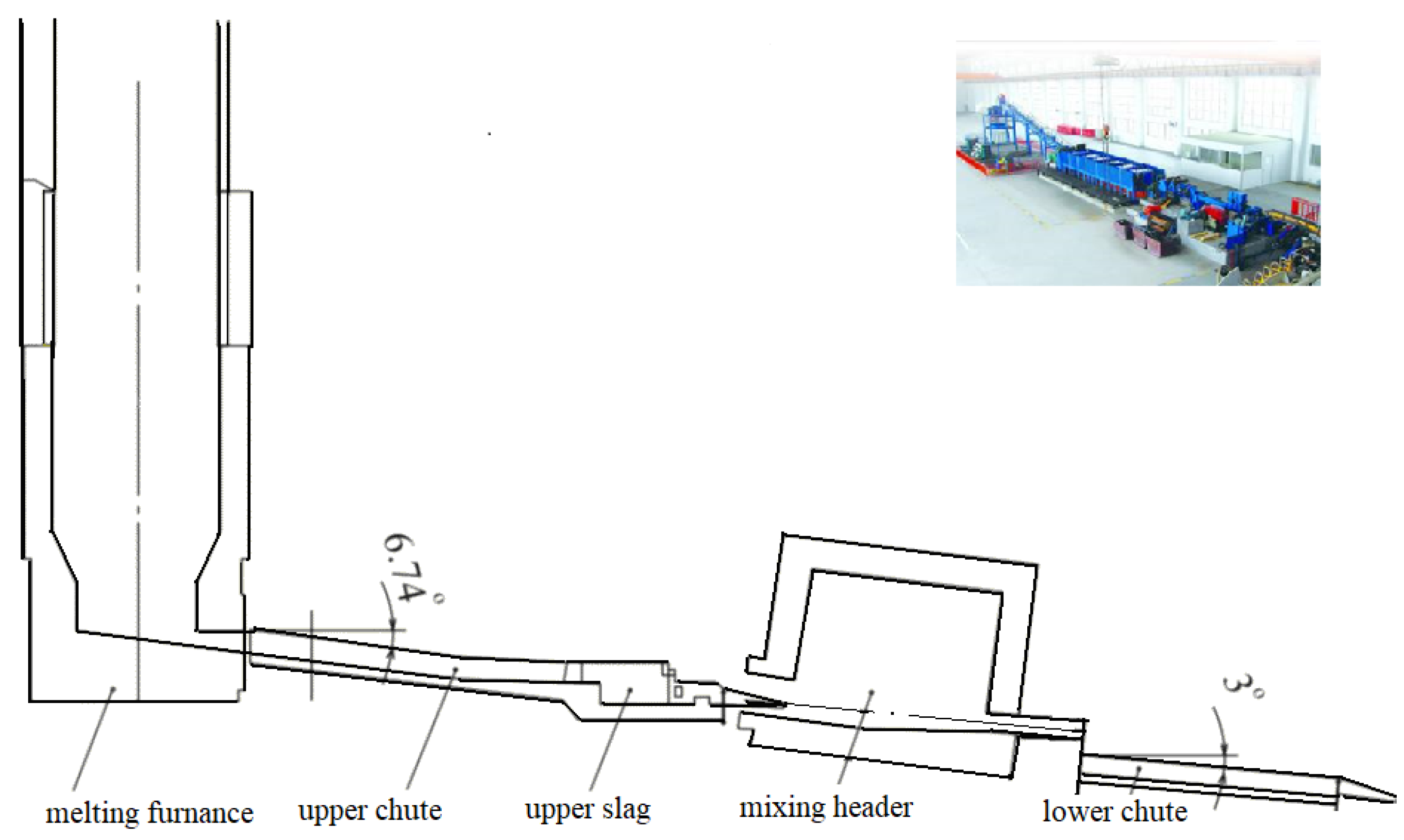
Our proposed physical and mathematical model (16)-(17) is constructed for the SCR - 2000 process equipment in Figure 1.

The calculations are made for the lower chute with an inclination angle of 3º, as shown in Figure 1.

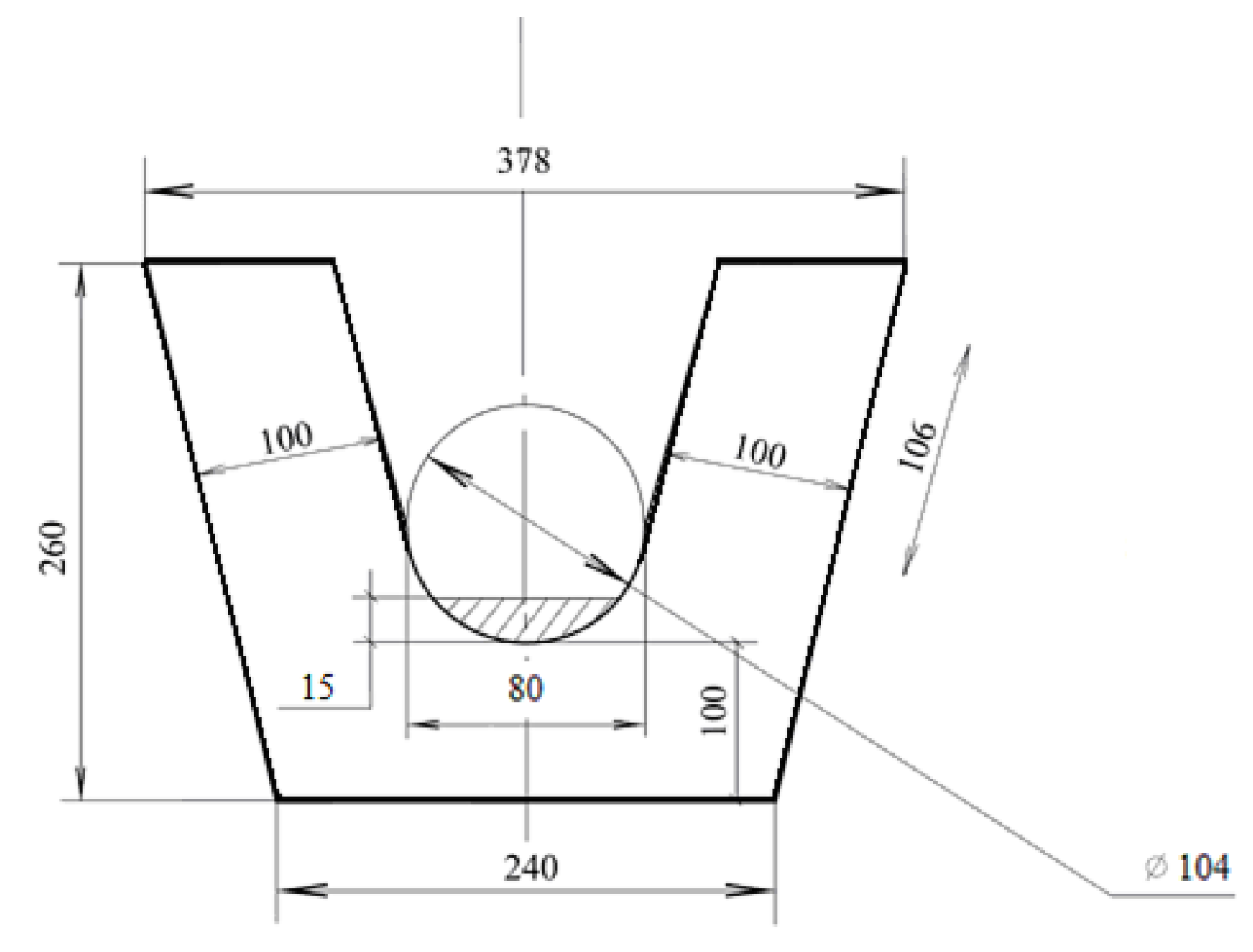
The metal melt level and the cross section of the lower chute are shown in Figure 2.

We calculated the numerical values of the melt flow parameters:

$S={\displaystyle \frac{\left[\lambda r-\sigma \left(r-h\right)\right]}{2}},$

$\lambda$ is arc length, $\sigma$ is chord, $h-$ is segment arrow:

$\sigma =80[\mathrm{mm}],h=16[\mathrm{mm}],\lambda \approx \sqrt{{\sigma }^2+\left(15h^2/3\right)}=\sqrt{{80}^2+\left(15\cdot {16}^2/3\right)}=87,6[\mathrm{mm}].$

$S={\displaystyle \frac{\left[87,6\cdot \frac{104}{2}-80\left(\frac{104}{2}-16\right)\right]}{2}}=1675,2[{\mathrm{mm}}^2].$

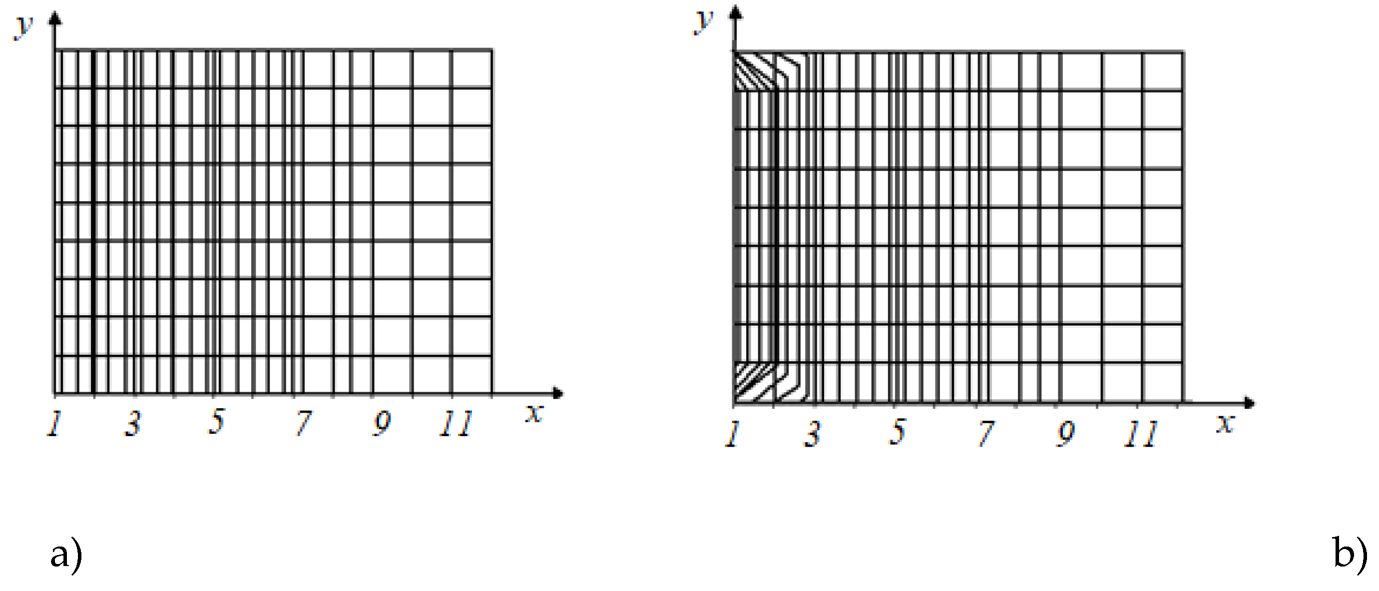
The average flow velocity of the metal melt is calculated by us according to the formula and is equal to ${\upsilon }_{ср}\approx 0,42\left[{\displaystyle \frac{\mathrm{m}}{\mathrm{s}}}\right].$ In the calculations of the numerical scheme $\Delta x=\Delta y=0,02.$ we used constant time step sizes $\Delta t=0,001.$ Calculated profiles of flow velocities $\upsilon$ and $u$ of metallic melt in the inclined trough Figure 2 equipment Figure 1 are shown in Figure 3.

Then the second melt flow velocity $q=3,6\left[{\displaystyle \frac{\mathrm{kg}}{\mathrm{s}}}\right]$is determined.

The adequacy of our calculations proves the effectiveness of the physical and mathematical model and its application to the calculation of the flow of metallic melts at sufficiently small Reynolds numbers.

The physical picture of copper melt flow in the process equipment is as follows: the different layers of melt do not mix with each other when travelling down the trough. The melt represents separate layers that move with different velocities increasing towards the melt surface. «From the moment atoms jump in the direction of the volumetric force, the flow is separated into a bottom layer and a main layer. The atoms of the bottom layer are held near the bottom surface by the interatomic coupling forces, while the atoms of the main layer move along the boundary of the bottom layer under the action of the bulk force. The walls of the trough due to internal friction inhibit the movement of the nearest copper melt layer, and this inhibition is transmitted from one layer to another throughout the melt flow to the surface, where the flow is the fastest» [9].

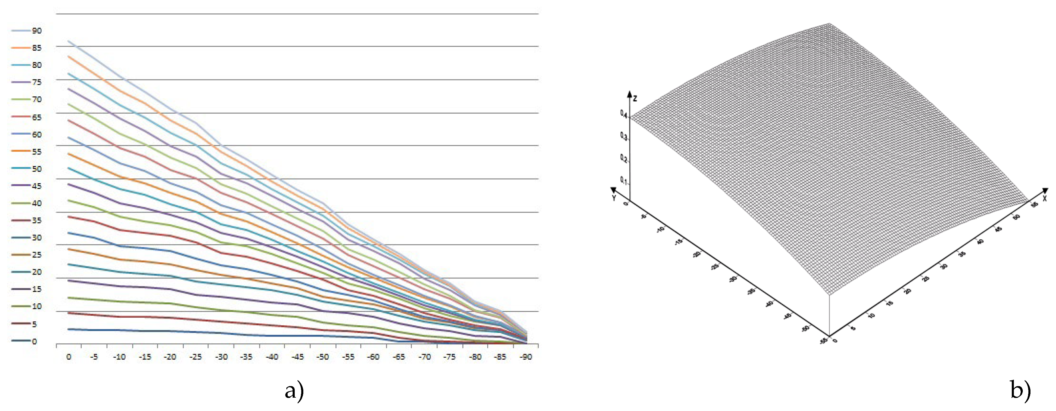
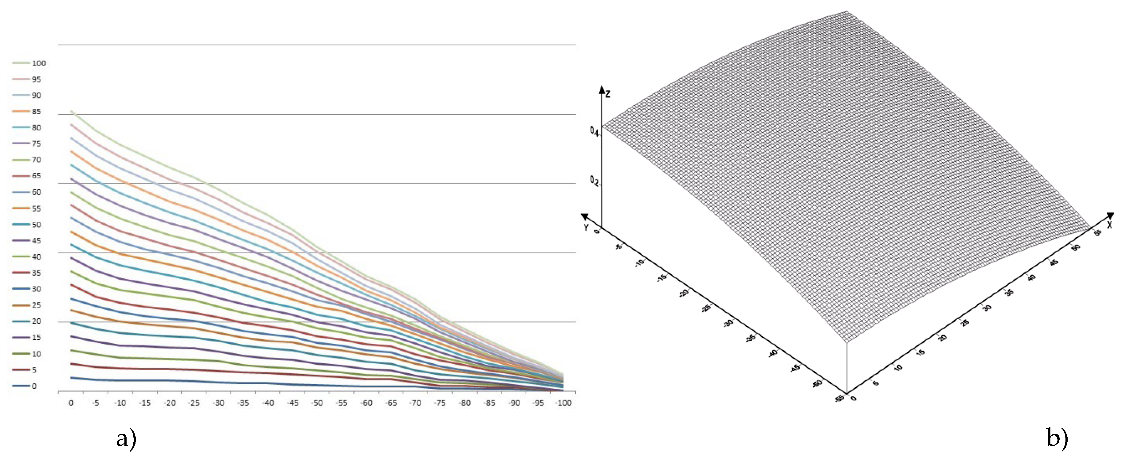
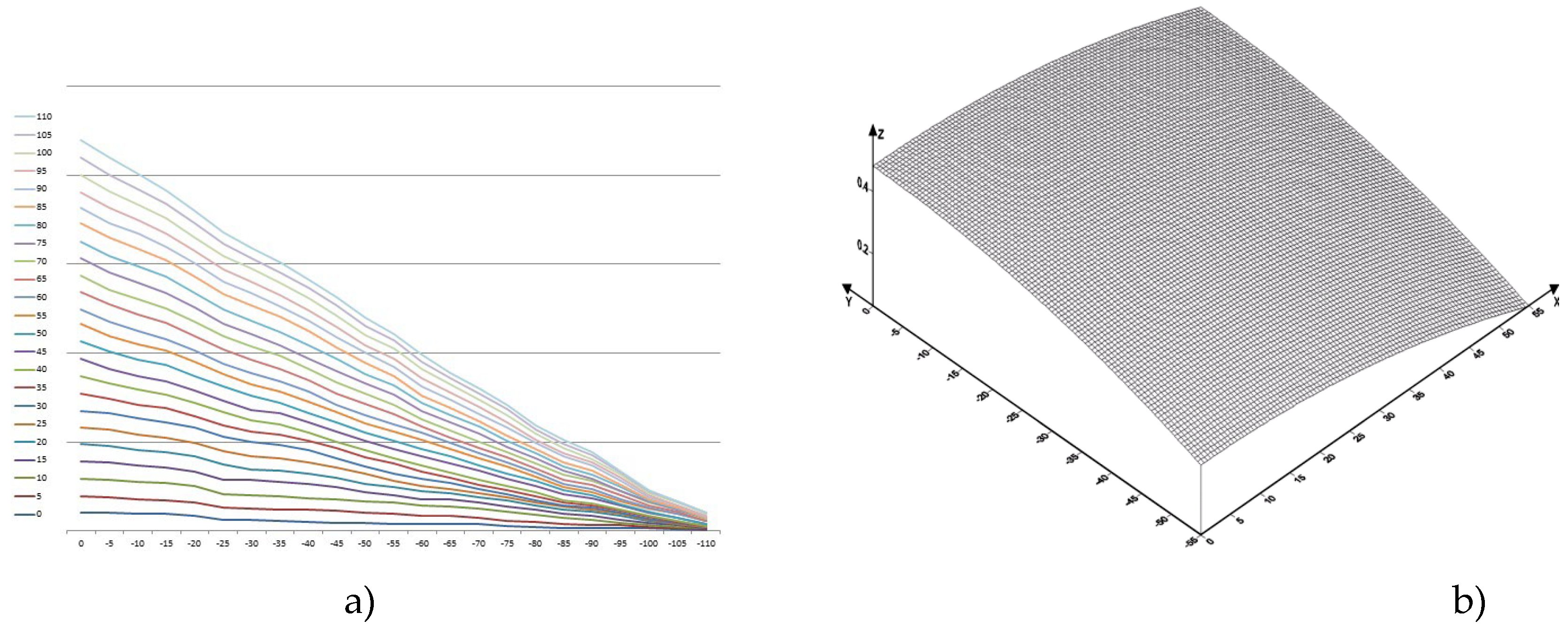
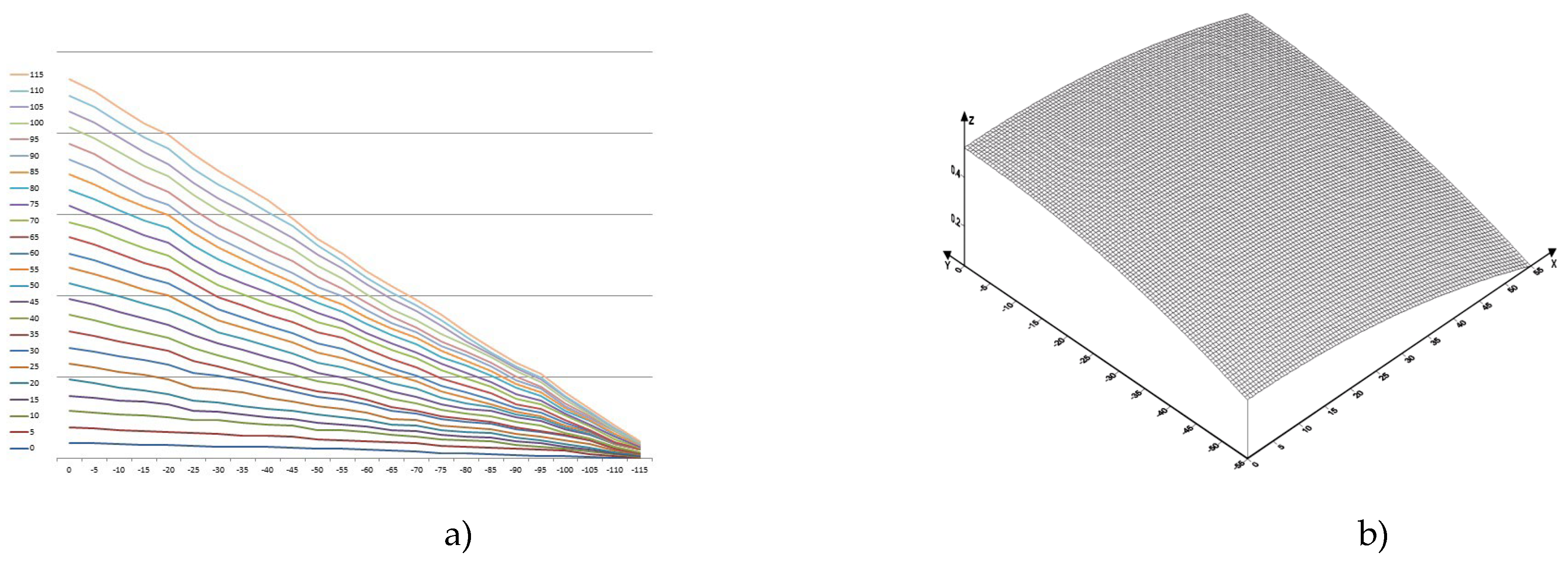
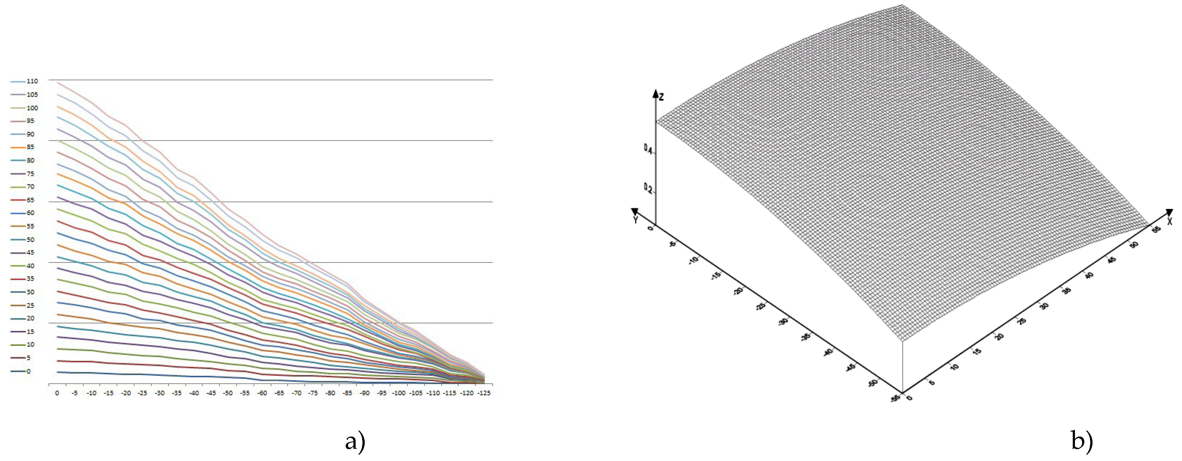
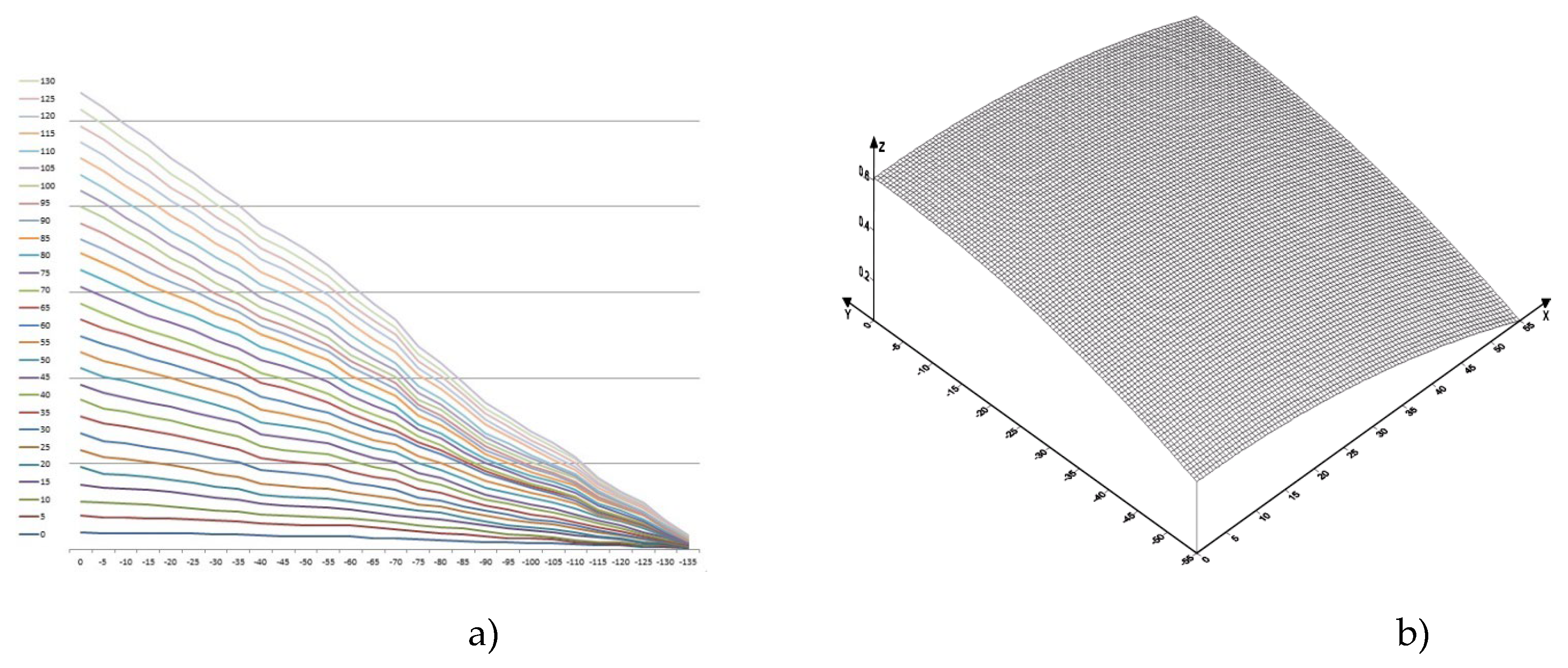
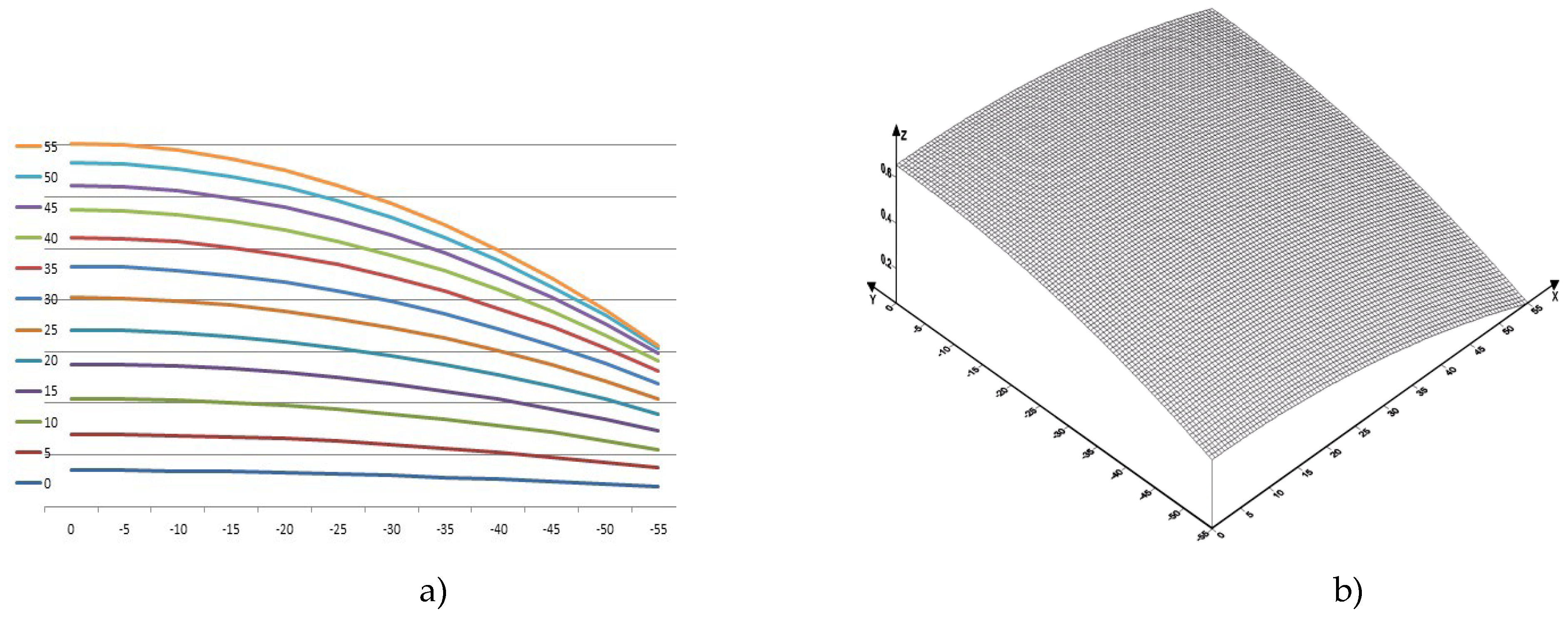
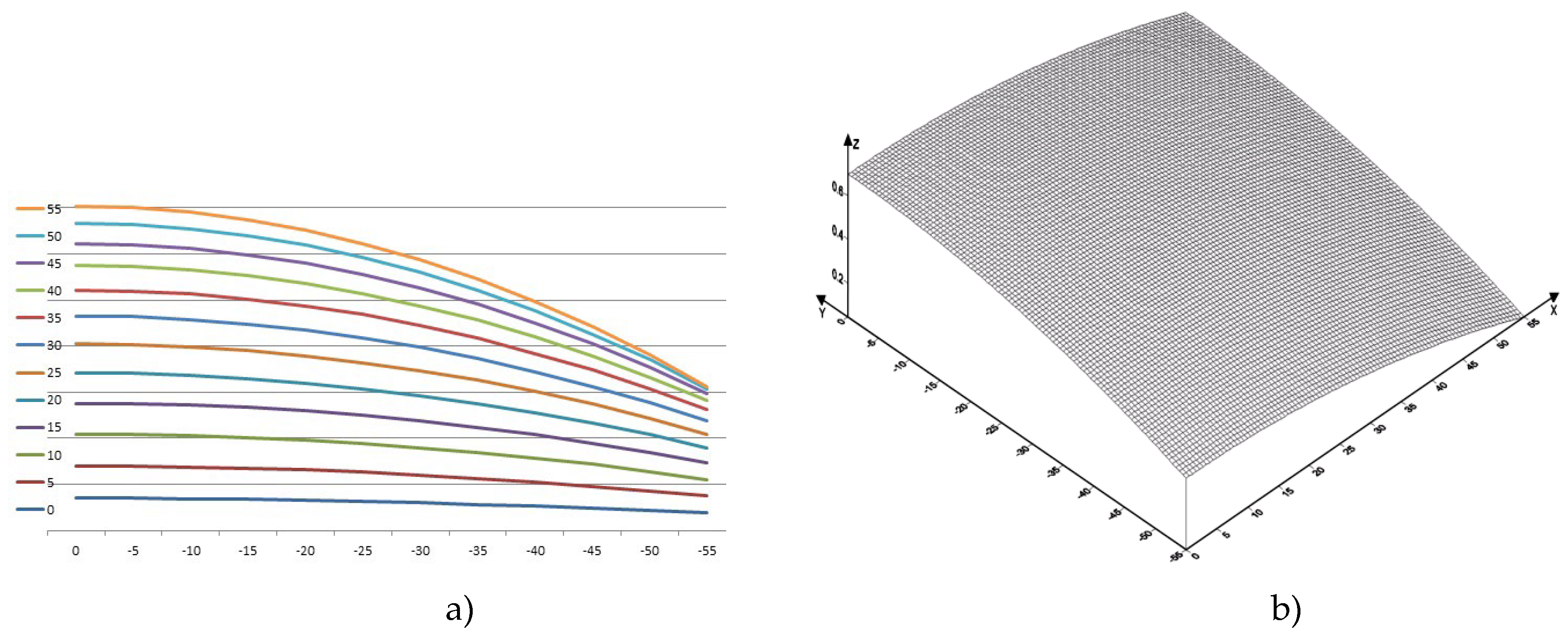
Let us consider the motion of copper melt taking into account shear and bulk viscosities. Profiles of copper flow velocity distribution profiles in the lower trough at temperatures 1357 [K], 1397 [K], 1437 [K], 1477 [K], 1517 [K], 1557 [K], 1597 [K], 1637 [K] in the plane in projections on XOY, as well as in space in the XYZ coordinate system are presented in Figure 4, Figure 5, Figure 6, Figure 7, Figure 8, Figure 9, Figure 10 and Figure 11 and in Table 1, Table 2, Table 3, Table 4, Table 5, Table 6, Table 7 and Table 8. The velocity isolines vary from $0,64\left[{\displaystyle \frac{\mathrm{m}}{\mathrm{s}}}\right]$ to $0,01\left[{\displaystyle \frac{\mathrm{m}}{\mathrm{s}}}\right]$. The mathematical model of melt motion is that the maximum velocity of melt motion is reached at the surface, at the bottom of the trough it is practically equal to zero, which is consistent with the boundary conditions of Equations (14) and (15). Calculations show that the average value of the velocity isoline is approximately equal to the average velocity of the copper melt flow $\upsilon \approx 0,4\left[{\displaystyle \frac{\mathrm{m}}{\mathrm{s}}}\right].$ Let us calculate the number of isolines at the specified temperatures:

T [K] 1357 1397 1437 1477 1517 1557 1597 1637

n is number of isolines 18 21 22 25 27 28 13 11

The maximum value of the isolines is observed at a temperature of 1557 [K]. The distribution of isolines is not dense at lower temperatures, e.g., at 1357 [K], as well as at high temperatures, e.g., at 1597 [K]. The calculations indicate the inhomogeneity of the melt near the melting temperature, which confirms the presence of melt cluster structure. Calculations also indicate inhomogeneity at temperatures of 1597 [K] and above, which is due to thermal loosening of the metallic melt structure and is the cause of mechanical defects in obtaining the intermediate product.

Verification of theoretical results with practical results of copper melted movement in the process equipment of the SOUTHWIRE - 2000 line at «Kazkat» in Zhezkazgan shows the adequacy of the our mathematical model, its objectivity and reliability.

We theoretically calculated the temperature of copper melt flow by numerical methods in the process equipment. Correctness and adequacy of our calculations are confirmed by verification with real temperatures of copper melted movement in the range 1423-1557 [K], which is close to the temperatures in industrial conditions.

5. Conclusions

We have developed a numerical scheme for regularisation of boundary value problems of the equations of motion of incompressible fluid. The complexity of solving these problems lies in the fact that the system of differential equations is non-evolutionary. The equation of motion of incompressible melt does not contain the time derivative of the pressure function. The approximation with the introduction of a small parameter in the original equation and the time derivative of the pressure function allowed us to pass from a non-evolutionary system of equations to an evolutionary one. In this paper, we have used Rothe's method to construct a numerical scheme of copper melt motion. The convergence of the solution of the approximating problem to the original boundary value problem of metallic melt motion was established. Verification of theoretical results with practical ones allowed to develop a mathematical model of melt motion and the numerical integration algorithm of hydrodynamic equations, which will allow to predict technological parameters of casting in order to obtain high-quality products. Validation of the obtained theoretical results with real parameters of copper melted movement in the process equipment of Southwier-2000 line confirms the validity and reliability of our research.

References

- R. Lakshminarayana, K. Dadzie, R. Ocone, M. Borg and J. Reese: Recasting Navier-Stokes equations. Journal of Physics Communications, 3(10), (2019), 13-18. [CrossRef]
- S.Sh. Kazhikenova, S.N. Shaltakov, D. Belomestny and G.S. Shaikhova: Finite difference method implementation for Numerical integration hydrodynamic equations melts. Eurasian Physical Technical Journal, 17(33), (2020), 50-56.
- Kazhikenova, S.Sh. The unique solvability of stationary and non-stationary incompressible melt models in the case of their linearization, Archives of Control Sciences, 31(LXVII), 307-302 (2021). [CrossRef]
- V. Shinde, E. Longatte, F. Baj, Y. Hoarau, M. Braza: A Galerkin-free model reduction approach for the Navier–Stokes equations. Journal of Computational Physics, 2016; 309. [CrossRef]
- A. Dumon, C. Allery, A. Ammar: Proper Generalized Decomposition method for incompressible Navier–Stokes equations with a spectral discretization. Applied Mathematics and Computation, 2013. [CrossRef]
- S. Hijazi, M. Freitag, N. Landwehr: POD-Galerkin reduced order models and physics-informed neural networks for solving inverse problems for the Navier–Stokes equations. Adv. Model. and Simul. in Eng. Sci, 2023. [CrossRef]
- Lorenzi S, Cammi A, Luzzi L, Rozza G. POD-Galerkin method for finite volume approximation of Navier–Stokes and RANS equations. Computer Methods Appl Mech Eng, 2016; 311. [CrossRef]
- Stabile, G. , Rozza G. Finite volume POD-Galerkin stabilised reduced order methods for the parametrised incompressible Navier-Stokes equations. Computers Fluids, 2018; 173. [Google Scholar] [CrossRef]
- E. Sciubba: A variational derivation of the Navier-Stokes equations based on the exergy destruction of the flow. Journal of Mathematical and Physical Sciences, 1991; 25, 61–68.
- Yun-hua Weng, Tao Chen. Xue-song Li, Nan-jing Huang: Rothe method and numerical analysis for a new class of fractional differential hemivariational inequality with an application. Computers & Mathematics with Applications, 2021; 98, 128–138. [CrossRef]
- Krzysztof Bartosz, Mircea Sofonea. The Rothe Method for Variational-Hemivariational Inequalities with Applications to Contact Mechanics. SIAM Journal on Mathematical Analysis, 2016; 48. [CrossRef]
- Xie X, Mohebujjaman M, Rebholz LG, Iliescu T. Data-driven filtered reduced order modeling of fluid flows. SIAM J. Sci. Computing, 2018; 40. [CrossRef]
- N.B. Iskakova, A.T. Assanova and E.A. Bakirova: Numerical method for the solution of linear boundary-value problem for integrodifferential equations based on spline approximations. Ukrains’kyi Matematychnyi Zhurnal, 71(9), (2019), 1176-91, http://umj.imath.[K]iev.ua/index.php/umj/article/view/1508.
- S.L. Skorokhodov and N.P. Kuzmina: Analytical-numerical method for solving an Orr-Sommerfeld type problem for analysis of instability of ocean currents. Zh. Vychisl. Mat. Mat. Fiz, 2018. [CrossRef]
- Ballarin F, Manzoni A, Quarteroni A, Rozza G. Supremizer stabilization of POD-Galerkin approximation of parametrized steady incompressible Navier-Stokes equations. Int J Numer Methods Eng. 2014. [CrossRef]
Figure 1.
- Diagram of the process equipment of the SOUTHWIRE - 2000 line.
Figure 2.
- Section of lower chute (measurements given in [mm]).
Figure 3.
(a) transverse and (b) longitudinal melt flow velocity profiles.
Figure 4.
The isolines at 1357 [K] temperature of a) – velocity, b) – surface.
Figure 5.
The isolines at 1397 [K] temperature of a) – velocity, b) – surface.
Figure 6.
The isolines at 1437 [K] temperature of a) – velocity, b) – surface.
Figure 7.
The isolines at 1477 [K] temperature of a) – velocity, b) – surface.
Figure 8.
The isolines at 1517 [K] temperature of a) – velocity, b) – surface.
Figure 9.
The isolines at 1557 [K] temperature of a) – velocity, b) – surface.
Figure 10.
The isolines at 1597 [K] temperature of a) – velocity, b) – surface.
Figure 11.
The isolines at 1637 [K] temperature of a) – velocity, b) – surface.