Submitted:
24 December 2024
Posted:
25 December 2024
You are already at the latest version
Abstract
The Yanguan Ancient Seawall, located at the Qiantang River estuary, is a nationally protected cultural heritage site and an in-service vital flood defense structure. Construction activities, including vehicle crossings, pose risks of vibration-induced damage. This study developed a three-dimensional finite element model to evaluate the vibration effects of moving vehicles on the Yanguan Ancient Seawall. The model captured the seawall's unique discrete-continuum structural characteristics by representing rubble stones with solid elements and sticky rice mortar with cohesive zone elements. Additionally, a Vehicle-Road Interaction element, capable of modeling vertical and tangential wheel-road contact forces, was implemented via the ABAQUS User Element interface. Field vibration tests validated the proposed methodology, demonstrating its reliability and accuracy. The validated model was applied to predict and analyze vibration responses under varying approach slab inclination angles, which contributes to the preservation of cultural heritage structures by providing scientific evidence to guide vibration protection measures.
Keywords:
Qiantang River ancient seawall
; Numerical simulation
; Vehicle-induced vibrations
; Vibration mitigation
; Finite element modeling
; Cultural heritage preservation
1. Introduction
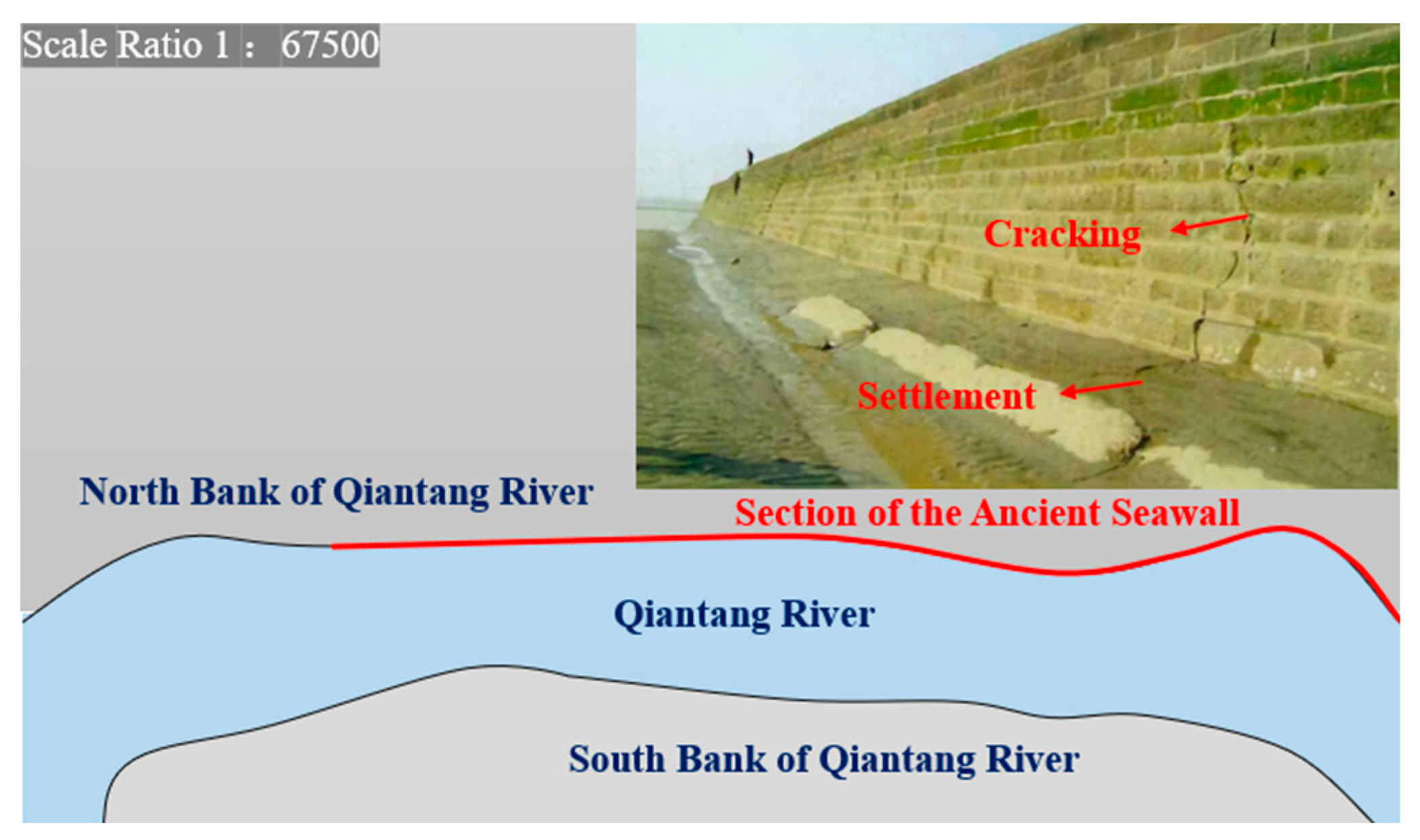
The seawalls along the Qiantang River serve as critical flood defense structures in the estuary region, protecting against tidal surges, typhoons, storm surges, and flooding events. Over time, these ancient seawalls have experienced significant structural degradation due to the combined effects of evolving natural conditions [1,2], intensive human activities [3,4], and the high-energy tidal bores characteristic of the Qiantang River [5]. Such factors have led to breaches in embankments and the destruction of protective aprons, thereby compromising the functional integrity of many seawall sections.
To address these challenges, the Zhejiang Province government in China initiated the “Billion Seawalls Reinforcement Project,” prioritizing the Yanguan ancient seawall segment along the Qiantang River. This large-scale initiative aims to upgrade the Yanguan seawall's flood defense standard from a 100-year to a 300-year return period. The reinforcement process involves several construction activities, including the installation of approach slabs spanning the seawall and vehicle crossings behind structure. However, dynamic loads generated by construction vehicles may induce excessive vibrations in the ancient seawall, posing risks of structural deterioration, such as cracking and severe damage to this nationally protected cultural relic.
Figure 1.
Structural issues in the Yanguan ancient seawall section along the Qiantang River.
Research on the vibration and deformation of historical structures has primarily focused on the effects of seismic and traffic loads on ancient buildings. For instance, Calik et al. [6] evaluated the seismic safety of a masonry mosque with a wooden truss roof, highlighting the significance of natural frequencies and damping ratios under environmental vibrations. Bayraktar et al. [7] assessed the effectiveness of restoration work on a stone masonry spire by comparing its dynamic characteristics before and after restoration. Ali et al. [8] identified structural improvements, such as vertical members and relatively thin horizontal bands, that enhance the seismic performance of rubble masonry houses through shaking table tests. Li et al. [9] investigated the vibration response of ancient buildings caused by subway operations, finding that the dynamic response amplitude induced by subway operations was ten times greater than that caused by road traffic. Kowalska-Koczwara et al. [10] measured the vibration response of St. Nicholas Church and proposed vibration protection measures. However, limited research has been conducted on nationally protected relics like the Qiantang ancient seawall, which serve dual roles as cultural relics and operational flood and tide defense structures. Existing studies primarily address the impact of pile-driving construction on the vibration and deformation of ancient seawalls, leaving a significant gap in understanding vehicle-induced vibrations during reinforcement activities.
The Qiantang ancient seawall is a masonry structure composed of rigid stone blocks bonded locally with sticky rice mortar, classifying it as a gravity retaining wall. While the stone blocks exhibit discrete characteristics, the overall wall structure demonstrates continuum behavior. This unique combination of discrete and continuous characteristics complicates the analysis of the seawall’s deformation and vibration. Conventional methods based solely on continuum or discrete media theories are insufficient for directly predicting its dynamic behavior. For masonry structures with such discrete-continuous characteristics, researchers often employ decoupled modeling approaches to develop finite element models. Page [11] first propose a decoupled finite element model for clay brick masonry. Lotfit et al. [12] introduced the use of zero-thickness interface elements to simulate mortar joints. Building on Lotfit's work, Lourenço et al. [13] combined blocks with half the thickness of their mortar joints and represented them using continuum elements. Andreotti et al. [14] adopted a decoupled modeling approach, using continuum elements for masonry walls and zero-thickness bonding interfaces for mortar, successfully simulating damage mechanisms and failure phenomena at mortar joints.
Despite these advancements, limited studies have investigated the impact of vehicle-induced vibrations on the structural integrity of ancient seawalls. There is currently no precedent for assessing the vibration effects caused by moving vehicles during the reinforcement and upgrade of such structures. Consequently, it is essential to develop an analysis method that incorporates the key characteristics of moving vehicle loads and the discrete-continuous nature of the ancient seawall structure.
In this study, solid elements and cohesive zone elements were employed to discretize the stone blocks and sticky rice mortar of the ancient seawall, respectively. A 3D finite element model reflecting the discrete-continuous structural characteristics of the seawall was developed using the general-purpose finite element software ABAQUS. Additionally, a vehicle-road coupled element capable of considering vertical and tangential wheel-road contact forces was implemented via the ABAQUS User Element (UEL) interface. This approach resulted in a 3D numerical analysis method capable of predicting the vibration effects of moving vehicles on the ancient seawall. The study also evaluated the vibration response levels of the seawall under different inclination angles of the approach slab spanning the seawall crest, providing scientific evidence for the vibration protection of cultural relics.
2. Measured vibrations of the ancient seawall induced by approach slab crossing
In the transverse direction of the ancient seawall, a steel trestle bridge extends into the river for soil excavation. To avoid direct vehicle loading on the ancient seawall crest, an approach slab is installed between the trestle bridge and the road behind the seawall. However, the vibrations induced by vehicles crossing the approach slab propagate to the ancient seawall, potentially compromising its structural stability. This section focuses on measuring the vibration levels of the ancient seawall structure caused by vehicles traversing the approach slab.
As illustrated in Figure 2, two horizontal vibration velocity sensors and one vertical vibration velocity sensor are installed on the surface of the approach slab. Similarly, two horizontal sensors and one vertical sensor are placed on the top of the ancient seawall directly beneath the vertical plane of the approach slab.
A three-axle unloaded truck, with a total weight of 25 tons and an axle load of 10 tons, is selected for the test. It should be noted that the axle load of 10 tons refers to the load distributed across each axle. The vehicle's speed is controlled at 5 km/h, and its travel path aligns with the centerline of the approach slab. The speed of 5 km/h was selected to simulate typical slow-moving construction vehicles, which are common in reinforcement projects.
The time-history curves of the vertical vibration velocity (Z) and horizontal vibration velocities (X and Y) on the approach slab surface under the crossing condition are shown in Figure 3. The results indicate that the vibrations induced by the vehicle crossing are predominantly in the vertical direction, with the vertical vibration velocity significantly exceeding the horizontal components. Specifically, the peak vertical vibration velocity reaches 77.5770 mm/s, which is 17.25 times greater than the peak horizontal vibration velocity in the X direction (4.4985 mm/s) and 21.6 times greater than that in the Y direction (3.5910 mm/s). These ratios highlight the significant disparity between the vertical and horizontal vibration components, emphasizing the need to focus on mitigating vertical vibrations to protect the structural integrity of the seawall.
The time-history curves of the vertical vibration velocity (Z) and horizontal vibration velocities (X and Y) of the ancient seawall structure under the approach slab crossing condition are presented in Figure 4. The results reveal a significant increase in vibration velocities in all three directions, contradicting typical observations where vertical vibrations often dominate in similar scenarios. This anomaly suggests that specific structural or loading conditions may amplify horizontal vibrations. Notably, the peak vibration velocity in the horizontal X direction (1.4800 mm/s) is 30.52 times greater than that in the horizontal Y direction (0.0485 mm/s) and 4.45 times greater than that in the vertical Z direction (0.3324 mm/s). This finding highlights the vulnerability of the seawall to transverse vibrations, which could lead to structural degradation or failure over time if not mitigated.
3. Vehicle-road coupling element considering vertical and tangential wheel-road contact forces
During construction, vehicles crossing the approach slab operate at an inclined angle relative to the ground, resulting in significant tangential forces between the wheels and the road. To accurately model these interactions, a Vehicle-Road Interaction (VRI) element is required, which can simultaneously account for both vertical and tangential wheel-road forces. The derivation of the VRI element's governing equations is primarily based on the theoretical framework proposed by Yang[15].
As shown in Figure 5, the vehicle moves at a constant velocity on a beam. The vehicle is modeled as a multi-rigid-body system, consisting of two rigid mass blocks representing the vehicle body and another rigid mass block for the wheels. These two components are connected by a suspension system, which is modeled using springs and dampers. The mass, stiffness, and damping matrices of the vehicle model are denoted as , , and respectively. The finite element dynamic control equation for the vehicle’s motion can be expressed as:
where, represents the displacement vector of the vehicle, which can be decomposed as, where subscripts and denote the displacements of the vehicle body and wheels, respectively. The load vectorcan be further expressed as:
whereis the contact force vector between the tires and the road surface, is the coordinate transformation matrix, andrepresents external loads other than the contact forces.
3.1. vehicle-road coupling element
Based on the degrees of freedom of the vehicle body and wheels, Equation (1) can be rewritten as:
where, and represent external loads acting on the vehicle body and wheels, respectively. The first row of Equation (3) corresponds to the vibration control equation for the vehicle body, while the second row corresponds to that for the wheels. Since contact forces only act on the wheels, . Expanding the first row of Equation (3) yields:
where:
Letdenote the displacement increment from timeto. Using the Newmark time-step integration method, the acceleration, velocity, and displacement of the vehicle body atcan be expressed as:
where in the equations provided, the superscript denotes variables known at the current time step. The coefficients in the Newmark time-step integration method, determined by the parametersand, are as follows:
Substitute Equations (6)–(8) into Equation (4) yields:
where:
By solving Equation (11), the displacement incrementsatcan be obtained. Substituting this result back into Equations (6)– (8) provides the vehicle's vibration response at.
Substituting Equation (13) into Equations (6)– (8) provides the vehicle's vibration response at:
Substituting Equation (14) into the second row of Equation (3) (the wheel vibration control equation), the wheel-road contact force at can be expressed as:
where, the mass, damping, and stiffness matrices are defined as:
The equivalent load vectors are:
where:
From Equation (15), it is evident that the wheel-road contact forcedepends not only on the wheel vibration response at (, , and) and the external load, but also on the known quantities at time. Assuming the wheel remains in contact with the road, the relationship between the wheel displacementand the road surface displacement at the contact pointis:
where, is a transformation matrix with elements of 1 or 0. Substituting this into Equation (15) establishes the relationship between the contact force and the contact displacement:
where the contact force for the-th wheel/bridge deck at () can then be expressed as:
In summary, the vehicle-road interaction model presented here effectively incorporates both vertical and tangential forces, providing a comprehensive framework for understanding the complex dynamics between the vehicle and the road surface.
3.2. wheel-road contact force
The contact force expressed in Equation (21) directly acts on the road surface, which is discretized into Euler-Bernoulli (E-B) beam elements. Each-th beam element is assumed to experience only the-th contact force. The size of the beam elements must be adjusted so that each element interacts with at most one wheel. The vibration control equation for the-th E-B beam element is expressed as:
where, ,, are the mass, damping, and stiffness matrices of the-th E-B beam element; is the nodal displacement vector of the beam element at time; is the equivalent nodal external load vector at time; is the equivalent nodal load vector contributed by the contact forceat the current time step, defined as:
where, represents the tangential wheel-road contact force, whereis the coefficient of friction. is the Hermite interpolation function for the E-B beam element, which only has non-zero components for vertical degrees of freedom. All other translational and rotational degrees of freedom are set to zero. This assumes that the vertical contact force is distributed as vertical nodal loads without causing horizontal forces or bending moments at the nodes. Therefore, equation (23) can be rewritten as:
where, represents the interpolation function. For E-B beam elements, the nodal degrees of freedom include horizontal displacement, vertical displacement, and rotation. The two interpolation functions related to horizontal displacement are and, where . Thus:
Based on Equation (24), the equivalent nodal load vector can be expressed as:
where the subscriptdenotes interpolation functions determined by the contact point coordinates. The vertical interpolation functionis defined as:
where, represents the local coordinate of the wheel-road contact point within the current E-B beam element, andis the element length. Substituting Equation (21) into Equation (23), Equation (22) can be rewritten as:
where the superscript indicates structural matrices and load vectors influenced by the moving wheel. These are defined as:
Equation (28) represents the vibration control equation of the beam element incorporating the degrees of freedom of the vehicle (hereafter referred to as the VRI element). The contribution of the vehicle to the beam element is reflected in the structural matrices and equivalent load vectors on the right-hand side of Equation (28). As shown in Equations (29), these terms depend on the real-time positionof the wheel. Therefore, the variables marked with * must be updated in real time according to the wheel's position when forming the VRI element.
4. Numerical analysis model of the ancient seawall considering discrete-continuous characteristics
4.1. Contact elements and crack simulation
The ancient seawall is essentially a masonry structure composed of stone blocks. While the individual blocks exhibit discrete characteristics, the overall wall structure demonstrates continuum behavior. To account for these characteristics, a simplified decoupled modeling approach is adopted to establish the finite element analysis model of the ancient seawall. The masonry blocks are modeled individually, while the mortar layers are treated as contact elements acting between solid elements.
As shown in Figure 6, the "traction-separation model" in ABAQUS is used to describe the relationship between normal stress, shear stress, and relative displacement at the contact interface. The parameters of this model include , which represents the nodal separation at complete interface failure; , which denotes the nodal separation at the onset of interface damage; , the tensile strength of the mortar; andthe shear strengths of the mortar, and the shear modulus.
4.2. Finite Element Elements and Constitutive Models
The ancient seawall's stone blocks and contact interfaces are discretized using C3D8R elements for the stone blocks and COH3D8 elements for the cohesive contact interfaces, respectively. The stone block elements employ the Drucker-Prager model, while the constitutive behavior of the interface elements follows the linear damage evolution shown in Figure 6. To simulate the degraded mechanical properties of the interface, initial damage and damage evolution laws are defined in the contact properties. The material properties of the stone blocks and cohesive contact models are detailed in Table 1, Table 2 and Table 3. This combination of constitutive models ensures that both the discrete behavior of the blocks and the continuum behavior of the mortar layers are accurately represented.
4.3. Model development and mesh generation
The schematic diagram of the ancient seawall model is shown in Figure 7. The model features a trapezoidal cross-section in the transverse direction, with bottom width of the model is 3.84 m, the top width is 1.44 m, and the height is 5.44 m. The model extends 5.7 m along the longitudinal direction of the seawall that encapsulates five masonry cycles of the prototype, which ensures that the model captures the representative structural behavior of the seawall.
The stone blocks in the model are simulated using stretcher and header bonding. Each block is rectangular with a cross-sectional size of 380 mm × 320 mm. However, the model includes 18 different block lengths, which are detailed in Table 4, to reflect the variability in block dimensions observed in the prototype. Figure 8 illustrates the structural mesh of the ancient seawall and the cohesive zone model, which provides a detailed representation of the contact behavior between the blocks and mortar layers.
5. Simulation and validation of the approach slab crossing condition
5.1. Establishment of the approach slab crossing model
(1) Soil model behind the ancient seawall
As illustrated in Figure 9, a soil model measuring 5.7 m in length, 12 m in width, and 5.44 m in height is constructed. This model primarily focuses on studying the impact of the approach slab crossing on the structure of the ancient seawall, excluding the effects of the road behind the embankment. To simplify the analysis, only the properties of the fill soil are considered, as detailed in Table 5. The material property parameters for the soil model are presented in Table 6.
(2) Approach slab model
The approach slab is divided into four components: longitudinal beams, crossbeams, the plate surface, and bedding stones. The modeling and element divisions for each component are illustrated in Figures 10(a)–(d). The material property parameters for the longitudinal beams, crossbeams, steel plate, and bedding stones within the ABAQUS model are presented in Table 7.
(3) Overall Model
The individual components are assembled to form the complete approach slab structure, integrating with the subsurface soil and the ancient seawall, as shown in Figure 11. To accurately simulate the actual constraints between the seawall and the approach slab, the following boundary conditions are imposed: the bottom surfaces of the soil and ancient seawall are constrained in all six degrees of freedom; the lateral surfaces of both the soil and the seawall are constrained similarly; two degrees of freedom are constrained on the side surface of the bedding stone; one degree of freedom is constrained at the back surface of the soil; and all six degrees of freedom are constrained at the outer end of the approach slab.
5.2. Simulation of the approach slab crossing and comparison with measured results
By integrating the VRI elements into the approach slab crossing model, a simulation analysis is performed under a load condition of 10 t per axle and a vehicle speed of 5 km/h. Vibration velocities at the slab surface and the seawall top are extracted and compared with the on-site measured results. The vertical vibration velocity (Z) of the slab surface and the horizontal vibration velocity (X) at the seawall top are identified as the dominant directions of vibration. The simulation results for these two directions are compared with the measured results in Figure 12 and Figure 13. The comparison reveals that the trends and peak values of the ABAQUS simulation results closely align with the on-site measurements. This alignment demonstrates the feasibility and accuracy of the approach slab crossing model in capturing the dynamic behavior of the system under vehicular loading conditions.
6. Analysis of vibration levels under different approach slab angles
To account for actual site conditions, the vehicle configuration is maintained with an axle load of 10 t and a speed of 5 km/h. The approach slab angle is varied across four scenarios (3°, 4°, 5°, and 6°) to analyze the vibration response of the ancient seawall structure at different angles. The peak vibration velocities on the slab surface and seawall top under each condition are summarized in Table 8. It can be observed that, as the approach slab angle increases, the peak vibration velocity gradually rises until the angle reaches 6°, at which point the peak vibration velocity begins to decline. Vehicle-induced vibrations primarily cause vibrations in the slab surface along the horizontal X direction and vertical Z direction, with the vertical Z direction being the dominant vibration direction. The vibration peak velocity in the Z direction is significantly higher than that in the horizontal X and Y directions. On the seawall top, the horizontal X direction dominates the vibration response, with its peak vibration velocity exceeding those in the vertical Z and horizontal Y directions. This highlights the importance of horizontal vibrations in the dynamic behavior of the seawall.
The simulation of a 3° slab angle, combined with a vehicle axle load of 10 t and a speed of 5 km/h, is simulated to analyze the vibration velocity trends, as depicted in Figure 14. The results reveal that the slab surface vibration velocity peaks at the center of the plate, while the vibration velocity on the seawall top attains its maximum at approximately 3 seconds after the vehicle begins crossing the slab. This peak is attributed to the second and third axles of the vehicle successively move onto the slab, based on the vehicle’s speed and axle spacing. Following these initial peaks, the subsequent vibration velocities diminish, indicating that the impact of the vehicle-induced vibrations decreases over time. Furthermore, the overall vibration pattern observed at the seawall top is consistent with the behavior recorded on the slab surface, highlighting a strong correlation between the two structural components in their dynamic responses.
7. Conclusions
This study presents a three-dimensional numerical analysis method to assess the vibration effects induced by moving vehicles on the Yanguan ancient seawall during its upgrading and reconstruction as part of the Qiantang River seawall reinforcement project. The analysis specifically focuses on the approach slab crossing condition, a critical construction scenario. The methodology was validated against field-measured vibration data collected during the construction process. The primary conclusions of this study are as follows:
(1) A VRI element, capable of accounting for both vertical and tangential wheel-road contact forces, was successfully developed using the UEL interface in ABAQUS. This element was integrated into a three-dimensional finite element model of the ancient seawall. The model discretized rubble stones and sticky rice mortar using solid elements and cohesive zone elements, respectively, effectively capturing the discrete-continuum structural characteristics of the seawall's composition.
(2) A three-dimensional finite element model of the approach slab crossing condition was constructed and validated through a comparison with field-measured vibration results. The numerical simulation results closely aligned with the measured data, successfully replicating the observed trends and peak vibration values. This validation demonstrates the model's reliability in predicting the structural vibrations of the ancient seawall under construction-induced loads.
(3) The validated numerical model was used to simulate and predict the vibration responses of the ancient seawall under various parameters, including different axle loads, vehicle speeds, and approach slab angles. These simulations provided critical insights into vibration behavior and served as a basis for ensuring the structural safety of the seawall during construction. Furthermore, the findings also contribute valuable scientific evidence for heritage conservation, supporting the safe restoration and preservation of this historically significant structure.
References
- Pan C, Zeng J, Tang Z, et al. A study of sediment characteristics and riverbed erosion/deposition in Qiantang estuary [J]. Hydro-Science and Engineering, 2013(1): 1-7. (in Chinese).
- Yu X, Li L, Wu X. Numerical simulation and analysis on tidal inundation of northern plain in Qiantang River estuary under ultra-violent typhoon [J]. Yangtze River, 2010, 41(8): 14-17+50. (in Chinese).
- Zou Z, Shen Y. Influence of the reclamation project at Qiantang estuary on the hydrodynamics and water environment in Hangzhou bay [J]. Port & Waterway Engineering, 2017(1): 26-33. (in Chinese).
- Zheng Y, Chen Z, Zhang K, et al. Field test on earth pressure of ancient seawall with different backfills for Qiantang River [J]. Rock and Soil Mechanics, 2014, 35(6): 1623-1628. (in Chinese).
- Chen L, Pan C. Research on river bed regulation in strong tidal reaches of Qiantang river [J]. The Ocean Engineering, 2008(2): 96-101+111. (in Chinese).
- Calik I, Bayraktar A, Türker T, et al. Ambient vibration based-simplified frequency formulas for historical masonry stone mosques with timber truss roofs[J]. Journal of architectural conservation, 2020, 26(3): 247-264. [CrossRef]
- Bayraktar A, Calik I, Türker T, et al. Restoration effects on experimental dynamic characteristics of masonry stone minarets[J]. Materials and structures, 2018, 51(6): 141. [CrossRef]
- Ali Q, Khan A N, Ashraf M, et al. Seismic performance of stone masonry buildings used in the himalayan belt[J]. Earthquake spectra, 2013, 29(4): 1159-1181. [CrossRef]
- Li K, Liu W, Liu W, et al. Tests and analysis of metro-induced vibration effects on surrounding historic buildings[C]. Key technologies of railway engineering - high speed railway, heavy haul railway and urban rail transit. Beijing: china railway publishing house, 2010: 921-926.
- Kowalska-Koczwara A, Stypula K. Protection of historic buildings against environmental pollution of vibrations[C]. 1st international conference on the sustainable energy and environment development (seed 2016), Cedex A: 10. E D P Sciences, 2016: 00043. [CrossRef]
- Page A, W. Finite element model for masonry[J]. Journal of the structural division, 1978, 104(8): 1267-1285. [CrossRef]
- Lotfi H R, Shing P B. Interface model applied to fracture of masonry structures[J]. Journal of structural engineering, 1994, 120(1): 63-80. [CrossRef]
- Lourenço P B, Rots J G. Multisurface interface model for analysis of masonry structures[J]. Journal of engineering mechanics, 1997, 123(7): 660-668. [CrossRef]
- Andreotti G, Graziotti F, magenes G. Detailed micro-modelling of the direct shear tests of brick masonry specimens: the role of dilatancy[J]. Engineering structures, 2018, 168: 929-949. [CrossRef]
- Yang Y, Wu Y. A versatile element for analyzing vehicle–bridge interaction response[J]. Engineering structures, 2001, 23(5): 452-469. [CrossRef]
Figure 2.
Schematic diagram of measurement points for vibration monitoring during approach slab crossing.
Figure 2.
Schematic diagram of measurement points for vibration monitoring during approach slab crossing.
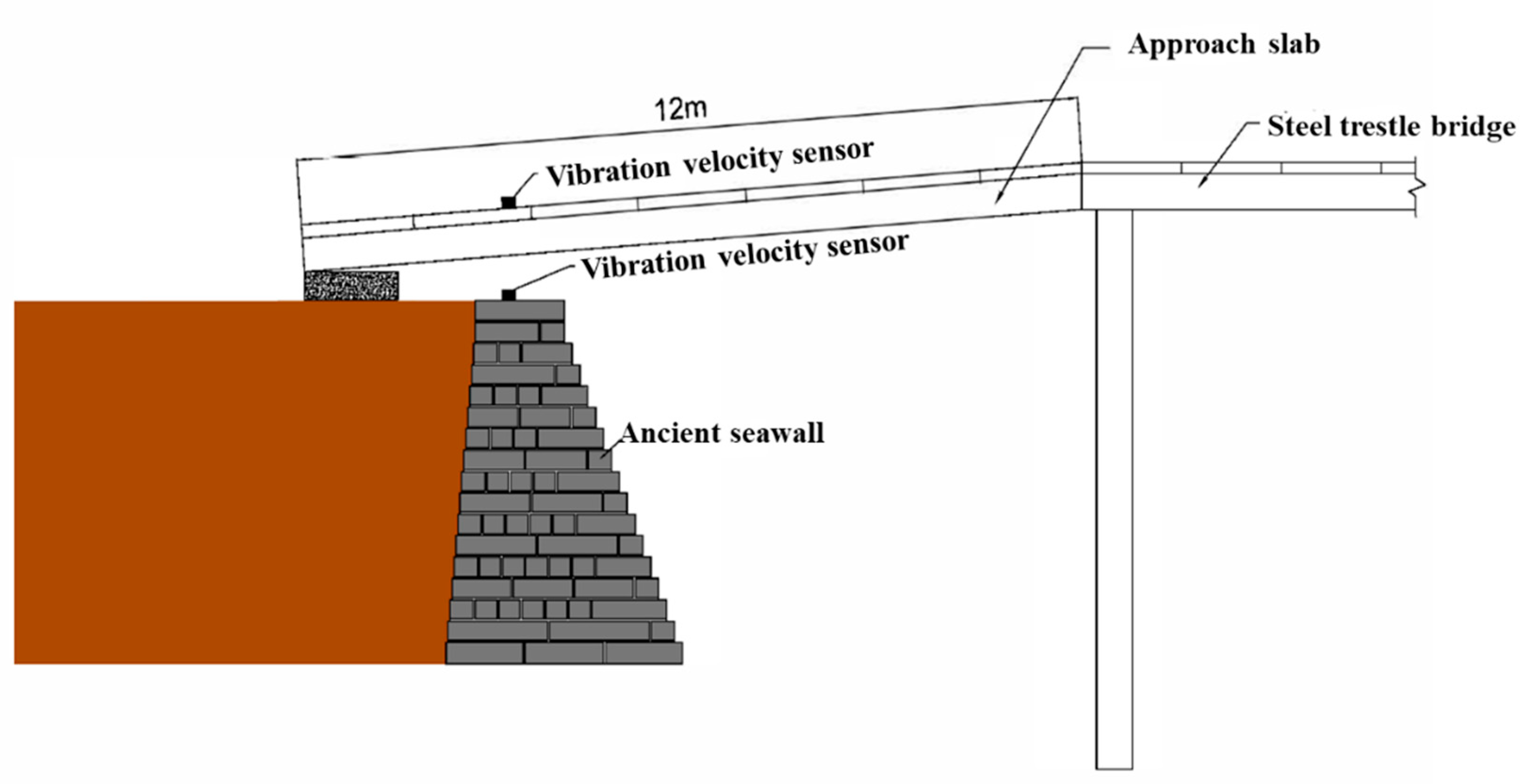
Figure 3.
Time-history curves of approach slab surface vibration under the crossing condition: (a) Horizontal direction X; (b) Horizontal direction Y; (c) Vertical direction Z.
Figure 3.
Time-history curves of approach slab surface vibration under the crossing condition: (a) Horizontal direction X; (b) Horizontal direction Y; (c) Vertical direction Z.
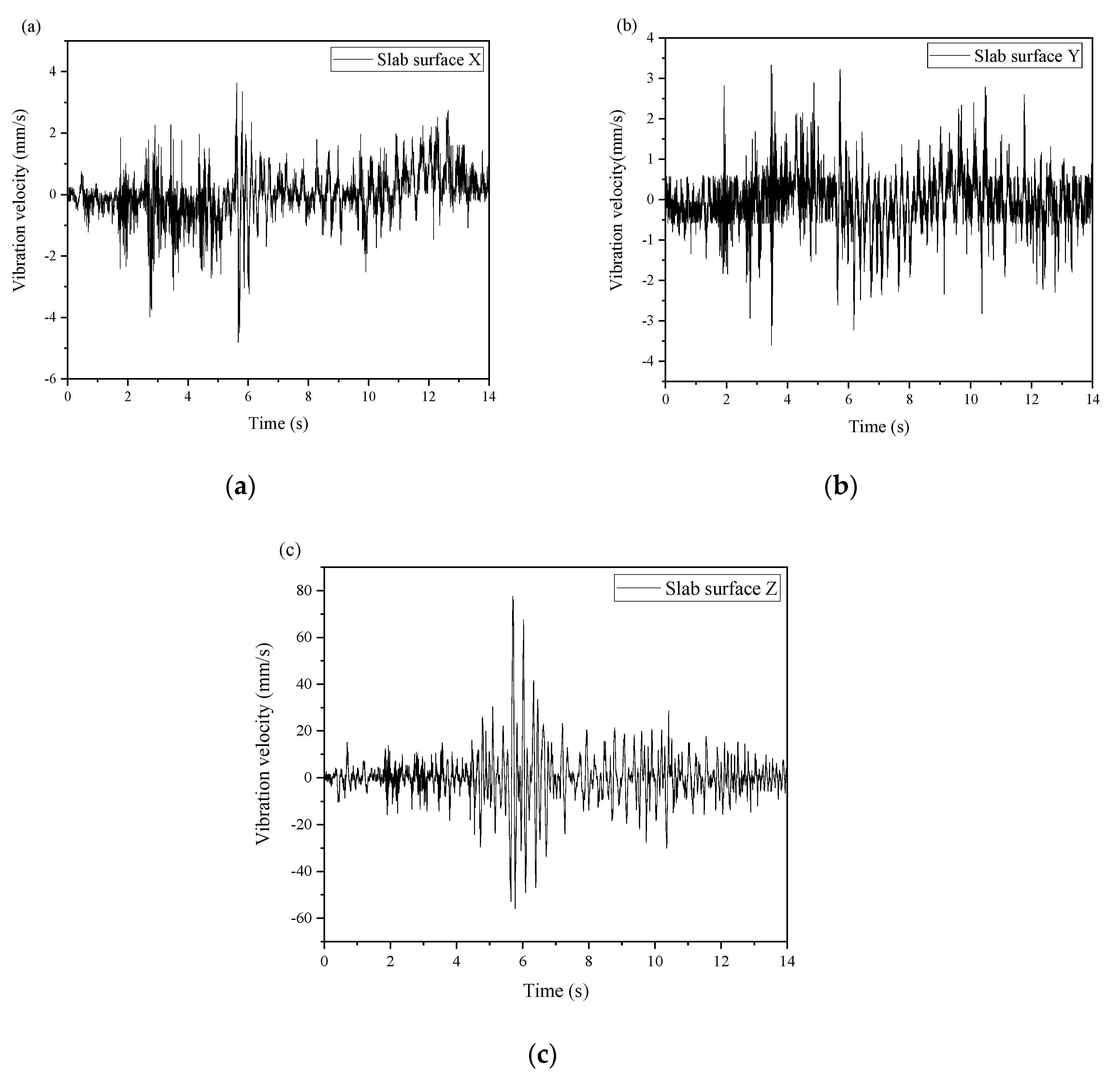
Figure 4.
Time-history curves of forced vibration of the ancient seawall top under the approach slab crossing condition: (a) Horizontal direction X; (b) Horizontal direction Y; (c) Vertical direction Z.
Figure 4.
Time-history curves of forced vibration of the ancient seawall top under the approach slab crossing condition: (a) Horizontal direction X; (b) Horizontal direction Y; (c) Vertical direction Z.
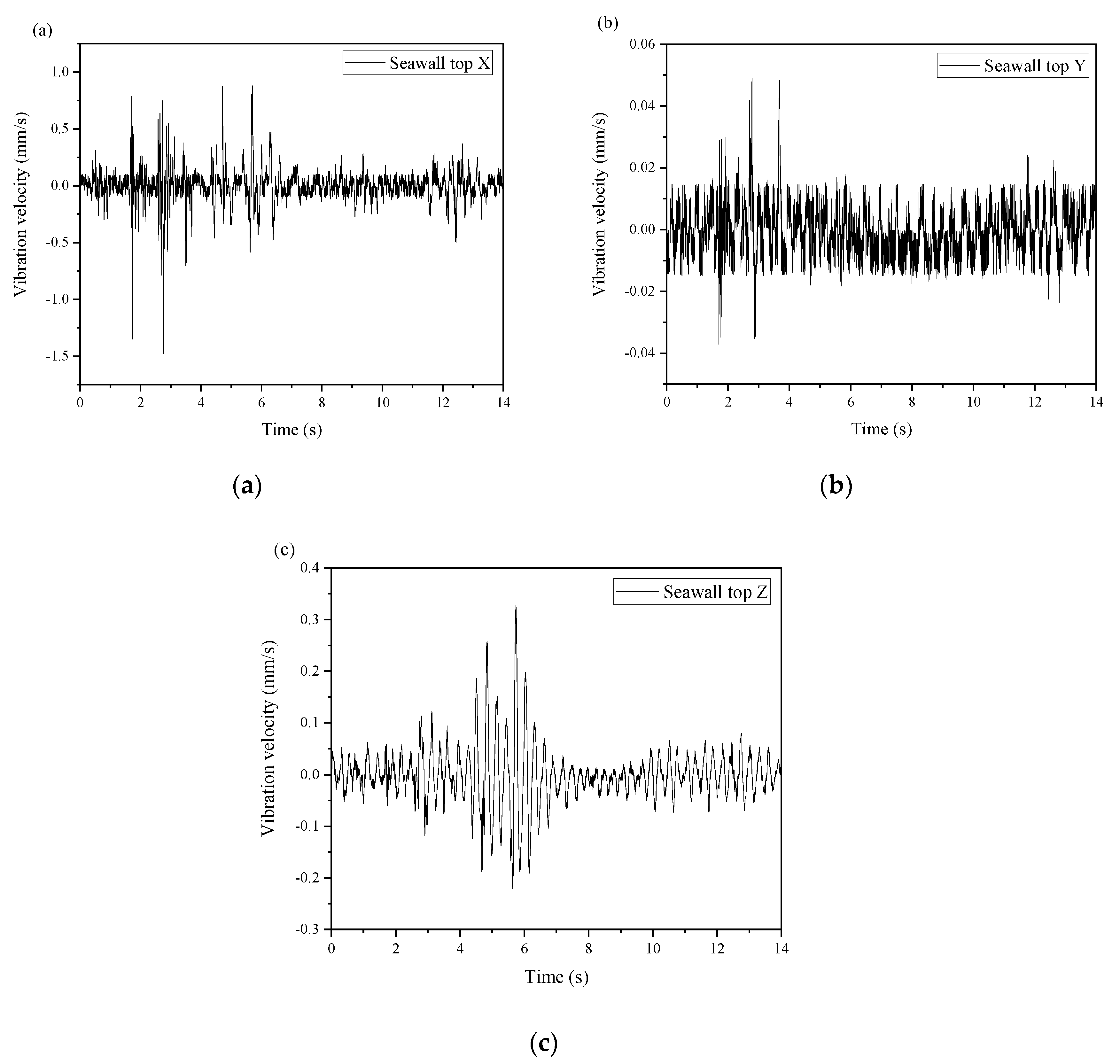
Figure 5.
Schematic of the vehicle-road coupling unit.
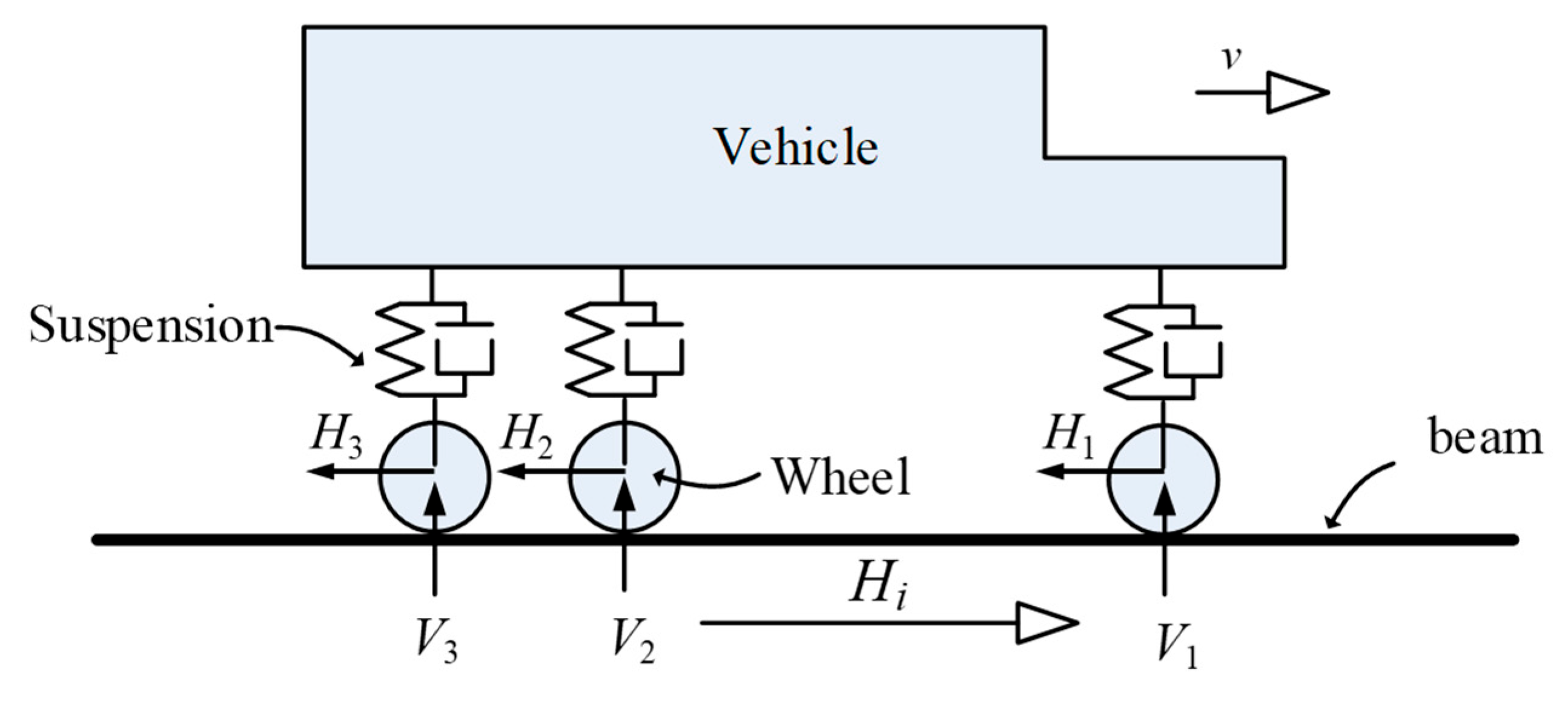
Figure 6.
Linear damage evolution in the traction-separation model.

Figure 7.
Schematic diagram of the model of the ancient seawall. (a) 3D illustration of the model dimensions, showing a longitudinal extension of 5.7 m. (b) Cross-sectional view of the model, showing a base width of 3.84 m, a top width of 1.44 m, and a height of 5.44 m.
Figure 7.
Schematic diagram of the model of the ancient seawall. (a) 3D illustration of the model dimensions, showing a longitudinal extension of 5.7 m. (b) Cross-sectional view of the model, showing a base width of 3.84 m, a top width of 1.44 m, and a height of 5.44 m.

Figure 8.
(a) Structural gridding of the ancient seawall; (b) Modelling of cohesive zones in the ancient seawall.
Figure 8.
(a) Structural gridding of the ancient seawall; (b) Modelling of cohesive zones in the ancient seawall.
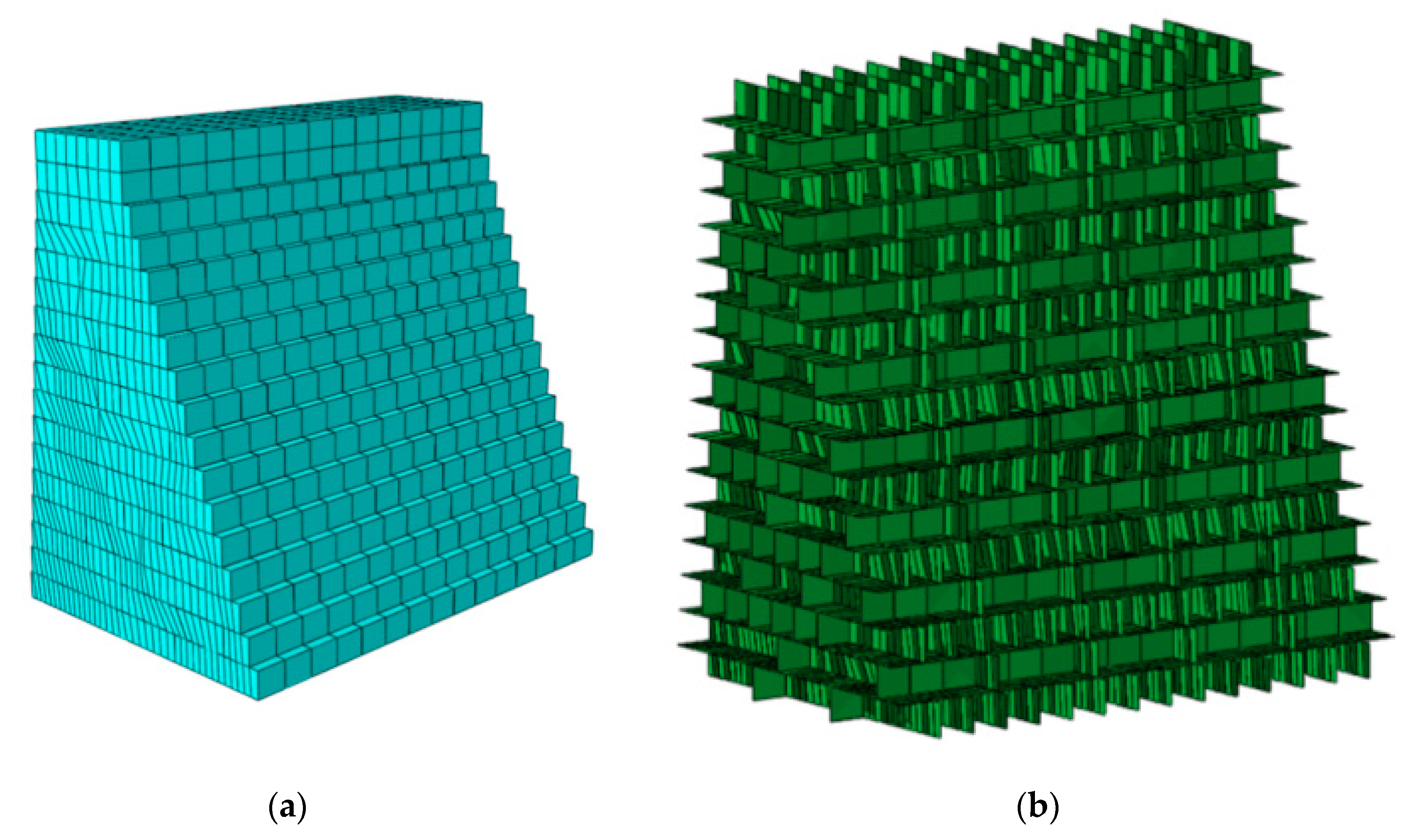
Figure 9.
Soil modeling behind the embankment.
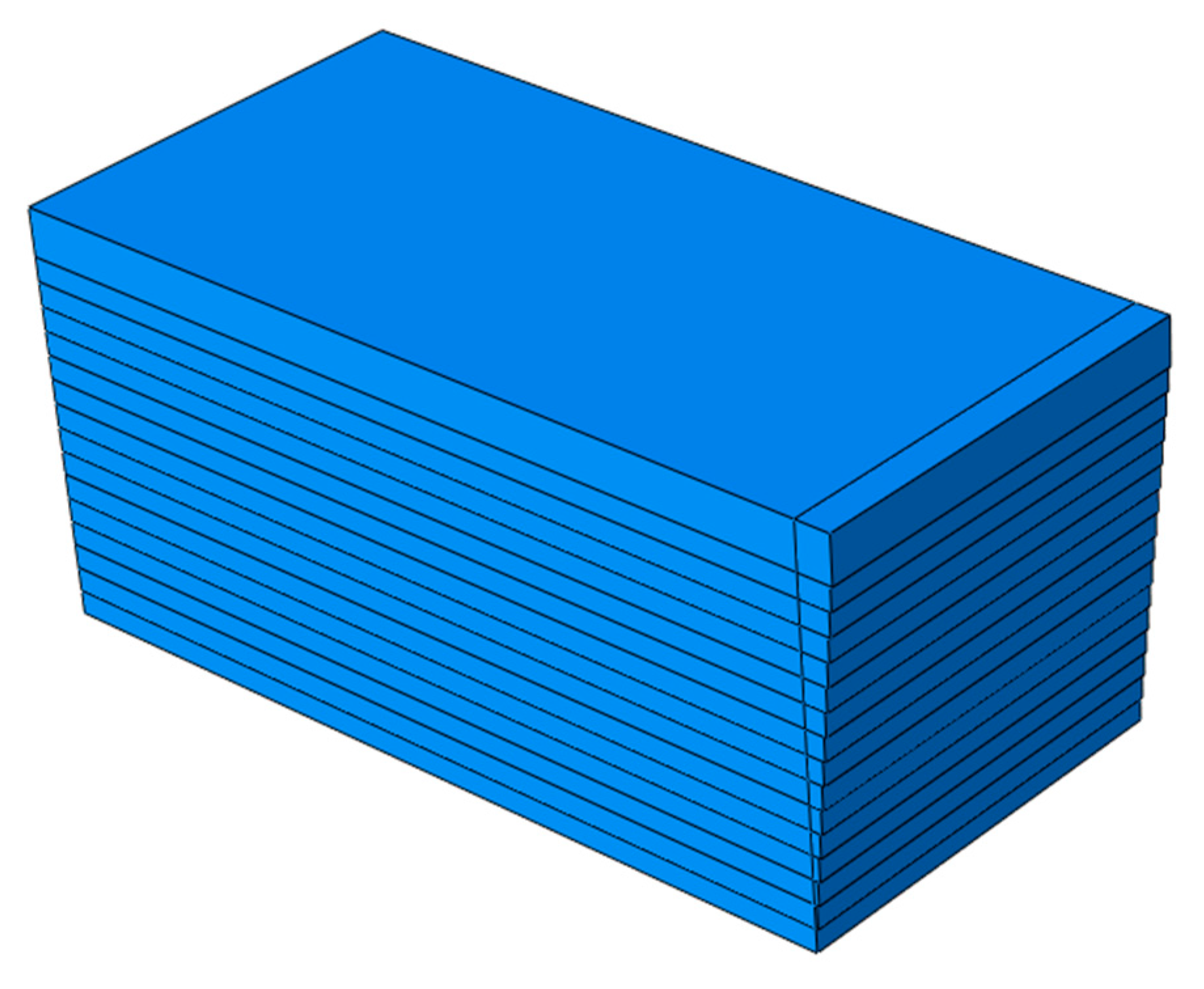
Figure 10.
(a) Longitudinal beam model; (b) Crossbeam model; (c) Plate model; (d) Bedding stone model; (e) Longitudinal beam meshing; (f) Crossbeam meshing; (g) Plate meshing; (h) Bedding stone meshing.
Figure 10.
(a) Longitudinal beam model; (b) Crossbeam model; (c) Plate model; (d) Bedding stone model; (e) Longitudinal beam meshing; (f) Crossbeam meshing; (g) Plate meshing; (h) Bedding stone meshing.
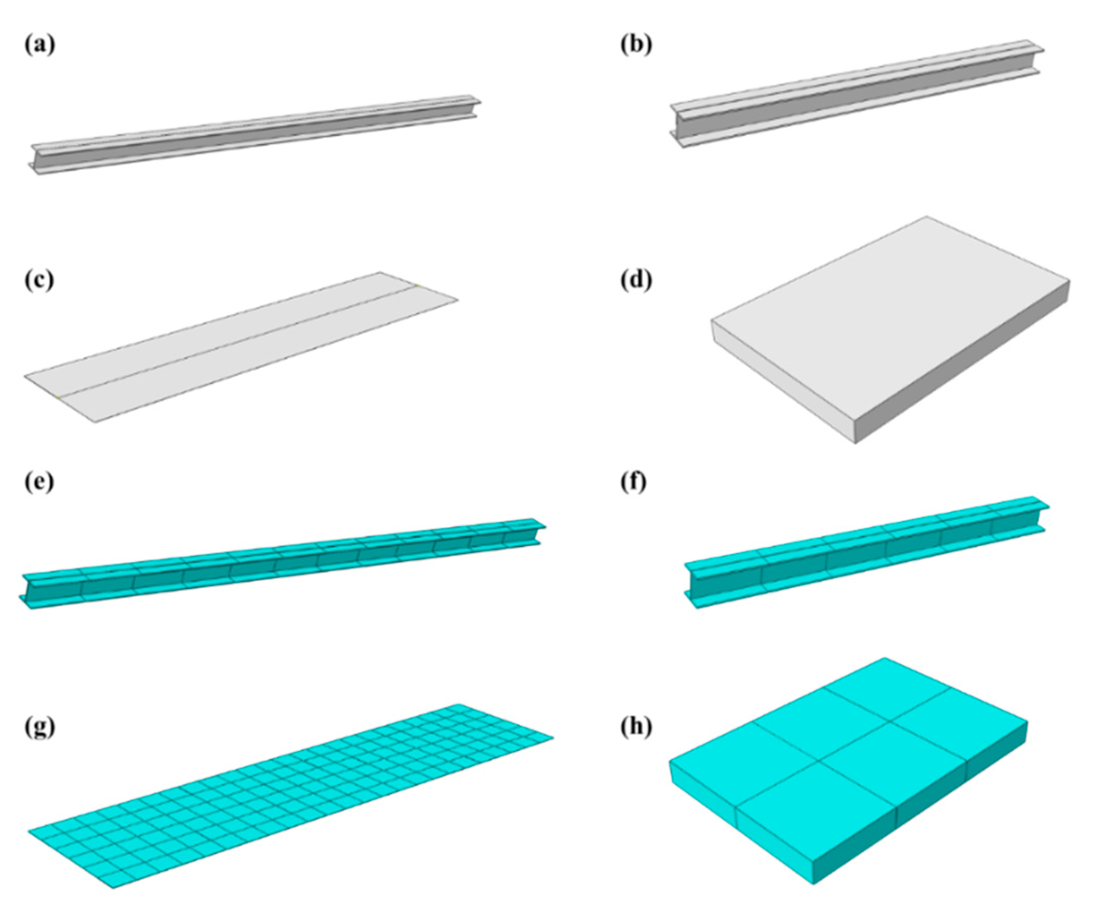
Figure 11.
Boundary condition settings for the approach slab crossing model.
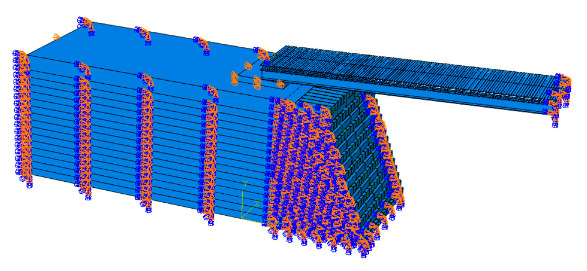
Figure 12.
Comparison of slab surface vibration simulation results with measured results (vertical direction Z).
Figure 12.
Comparison of slab surface vibration simulation results with measured results (vertical direction Z).
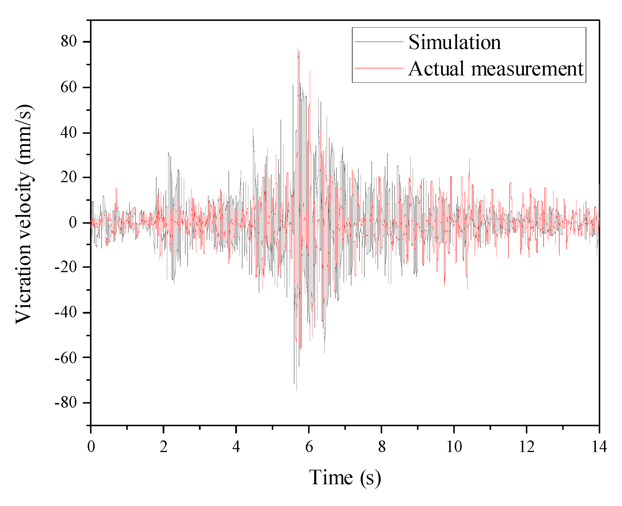
Figure 13.
Comparison of simulation results and measured results of vibration on seawall top (horizontal direction X).
Figure 13.
Comparison of simulation results and measured results of vibration on seawall top (horizontal direction X).
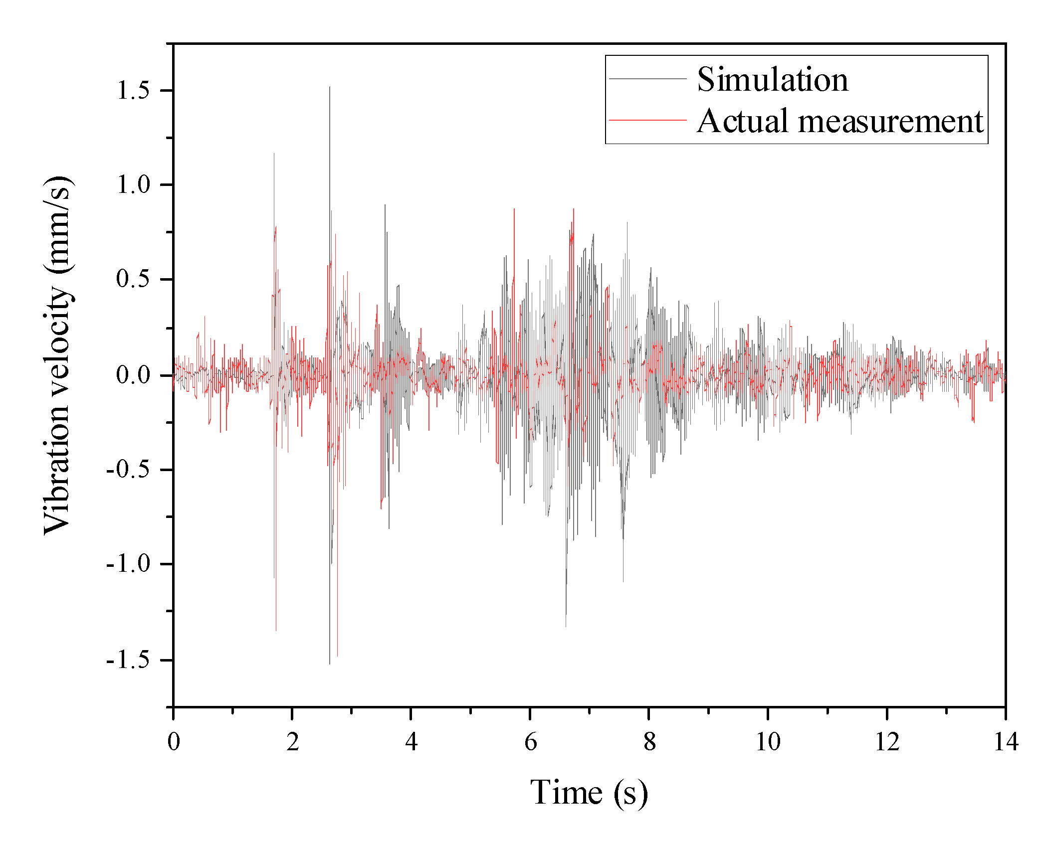
Figure 14.
Simulation results for a 10 t axle load, 5 km/h vehicle speed, and a 3° approach slab angle: (a) vibration velocity of the slab surface; (b) vibration velocity at the seawall top; (c) mortar strain at the seawall top.
Figure 14.
Simulation results for a 10 t axle load, 5 km/h vehicle speed, and a 3° approach slab angle: (a) vibration velocity of the slab surface; (b) vibration velocity at the seawall top; (c) mortar strain at the seawall top.
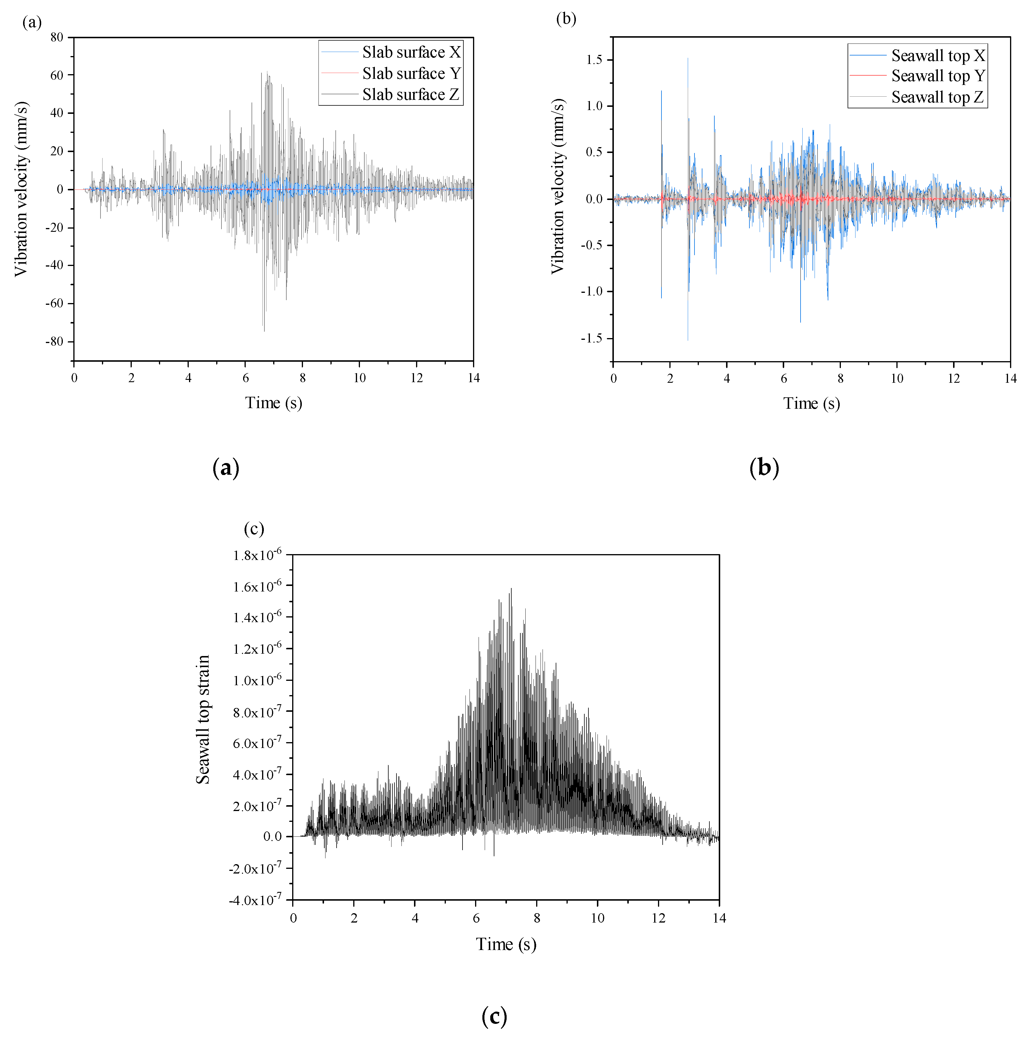

Table 1.
Material properties of the block layer in the ancient seawall structure.
| Density | Young’s Modulus | Poisson’s Ratio | Friction angle | Flow stress ratio | Dilation angle |
|---|---|---|---|---|---|
| 32.6 MPa | 0.2 | 53.47° | 1 | 16.72° |
Table 2.
Parameters of the plastic hardening material model for the stone blocks.
| Yield stress (MPa) | Absolute plastic strain |
|---|---|
| 62.28 | 0 |
| 78.78 | 0.0005 |
| 95.99 | 0.001 |
| 113.07 | 0.0015 |
| 130.3 | 0.002 |
| 145.87 | 0.0025 |
Table 3.
Material properties of the mortar layer for cohesive contact interfaces.
| Property | Value |
|---|---|
| Density | 1030 kg/m3 |
| 2.22×10⁹ Pa | |
| 9.1×10⁸ Pa | |
| 9.1×10⁸ Pa | |
| 3×10⁵ Pa | |
| Surface: 2.31×10⁵ Pa Middle: 2.47×10⁵ Pa Bottom: 2.57×10⁵ Pa |
|
| Normal fracture energy | 469 J/m2 |
| Shear fracture energy | 1210 J/m2 |
Table 4.
Length specifications of boulders in the ancient seawall model.
| Block type | Length (mm) | Block type | Length (mm) |
|---|---|---|---|
| (1) | 1440 | (10) | 1170 |
| (2) | 1060 | (11) | 980 |
| (3) | 840 | (12) | 1330 |
| (4) | 1380 | (13) | 920 |
| (5) | 780 | (14) | 993 |
| (6) | 850 | (15) | 1240 |
| (7) | 1100 | (16) | 1650 |
| (8) | 1010 | (17) | 1280 |
| (9) | 1040 | (18) | 1140 |
Table 5.
Physical and mechanical properties of the soil layer behind the embankment.
| Soil layer | Moisture content (%) | /m3) | Pore ratio) | Liquid limit | Plastic limit | |
|---|---|---|---|---|---|---|
| Fill soil | 26.9 | 18.8 | 2.71 | 0.786 | 30.6% | 19.0% |
Table 6.
Material property parameters of the soil model behind the embankment.
| Rayleigh Damping Parameters(Rev/min) | ) | Elastic modulus | Poisson's Ratio | |
|---|---|---|---|---|
| Fill soil | Alpha: 0.04 Beta: 6.96×10⁻⁵ |
1880 | Young’s Modulus:210 MPa Poisson's Ratio:0.25 |
0.2 |
Table 7.
Material property parameters for the components of the approach slab model.
| ) | Parameters | |
|---|---|---|
| Longitudinal beam | 7850 |
Poisson's Ratio: 0.3 |
| Crossbeam | 7850 |
Poisson's Ratio:0.3 |
| Steel plate | 7850 |
Poisson's Ratio:0.3 Coefficient of friction with wheels: 0.2 |
| Bedding stone | 2000 |
Poisson's Ratio: 0.2 |
Table 8.
Peak vibration velocities for an axle load of 10 t, vehicle speed of 5 km/h, and varying approach slab angles.
Table 8.
Peak vibration velocities for an axle load of 10 t, vehicle speed of 5 km/h, and varying approach slab angles.
| Condition | Vibration direction | ||
|---|---|---|---|
| Slab surface | Seawall top | ||
| Slab angle 3° | X | 13.1983 | 1.5203 |
| Y | 0.9616 | 0.1538 | |
| Z | 74.4949 | 1.1980 | |
| Slab angle 4° | X | 22.6205 | 1.7103 |
| Y | 1.7248 | 0.2960 | |
| Z | 81.0554 | 1.3477 | |
| Slab angle 5° | X | 36.4729 | 1.9003 |
| Y | 2.8869 | 0.3348 | |
| Z | 88.4512 | 1.4974 | |
| Slab angle 6° | X | 13.9938 | 1.0642 |
| Y | 0.5448 | 0.1414 | |
| Z | 80.8559 | 0.8386 | |
Disclaimer/Publisher’s Note: The statements, opinions and data contained in all publications are solely those of the individual author(s) and contributor(s) and not of MDPI and/or the editor(s). MDPI and/or the editor(s) disclaim responsibility for any injury to people or property resulting from any ideas, methods, instructions or products referred to in the content. |
© 2025 by the authors. Licensee MDPI, Basel, Switzerland. This article is an open access article distributed under the terms and conditions of the Creative Commons Attribution (CC BY) license (https://creativecommons.org/licenses/by/4.0/).
Copyright: This open access article is published under a Creative Commons CC BY 4.0 license, which permit the free download, distribution, and reuse, provided that the author and preprint are cited in any reuse.


