
Submitted:
23 December 2024
Posted:
24 December 2024
You are already at the latest version
Abstract
Efficient nitrogen management is crucial for improving corn productivity while minimizing environmental impacts. This study evaluates the response of corn to nitrogen fertilization using three key metrics: Yield, Nitrogen Harvest Index (NHI), and Agronomic Nitrogen Use Efficiency (ANUE). The experiment was conducted over three years (2021-2023) across 84 sites in Quebec, Canada, with five nitrogen treatments applied post-emergence (0, 50, 100, 150, 200 kg N/ha) and initial nitrogen applied at seeding (30 to 60 kg/ha). In addition, various soil health indicators, including physical, chemical, and biochemical properties, were monitored to understand their interaction with nitrogen use efficiency. Machine learning techniques, such as Augmented Extreme Learning Machine (AELM) and Particle Swarm Optimization (PSO), were employed to optimize nitrogen recommendations by identifying the most relevant features for predicting yield and nitrogen use efficiency (NUE). The results highlight that integrating soil health indicators such as enzyme activities (β-glucosidase [BG] and N-acetyl-β-D-glucosaminidase [NAG]) and soil proteins into nitrogen management models improves prediction accuracy, leading to enhanced productivity and environmental sustainability. These findings suggest that advanced data-driven approaches can significantly contribute to more precise and sustainable nitrogen fertilization strategies.
Keywords:
Augmented Extreme Learning Machine (AELM)
; Feature Selection
; Particle Swarm Optimization (PSO)
; Nitrogen Use Efficiency (NUE)
; Soil Health Indicators
; Corn Yield
1. Introduction
Efficient agricultural management practices are essential to ensure both high productivity and environmental sustainability, particularly in the context of nitrogen fertilization for crops such as corn. Corn (Zea mays L.), an important crop in Quebec, in terms of cultivated area and farm revenues. In 2020, 459,100 hectares were planted with corn (grain corn and silage corn). Nitrogen application rates are up to 240 kg/ha, significantly higher than the recommended maximum rate of 170 kg/ha [1]. This over-application of nitrogen has both economic and environmental consequences, necessitating more efficient nitrogen management strategies. Approximately 50% of the nitrogen applied is in the form of urea, which has a nitrous oxide (N₂O) emission factor of 1.1% of the applied amount [2]. This practice has a significant environmental impact, with a potential contribution of up to 100,000 tons of CO₂ equivalent emissions from corn fields in Quebec [2]. However, this estimate may be conservative, as nitrogen fertilization significantly increases N₂O emissions, especially when application rates exceed crop requirements, due to the exponential—rather than linear—relationship between nitrogen inputs and emissions [3,4].
The environmental consequences of excessive nitrogen fertilization extend beyond greenhouse gas emissions. Nitrogen losses occur through various pathways, including ammonia volatilization, denitrification, and nitrate leaching, leading to significant air and water pollution and soil degradation [5,6,7]. These losses are often not directly associated to a proportional increase in crop yield, highlighting the inefficiency of over-fertilization [5]. Recent studies have demonstrated that optimal nitrogen fertilization techniques, such as site-specific nutrient management, have reduced nitrogen application rates by 30-60% without sacrificing crop yields while substantially decreasing environmental impacts [8,9].
Although advancements in nitrogen management exist, there exists a pressing need to adequately incorporate soil health metrics into fertilization models. Indeed, despite significant advances in fertilization technologies, current nitrogen recommendation models often fail to account for the influence of soil health on crop response to fertilization. Soil health, which includes physical, chemical, biochemical, and microbiological properties, plays a critical role in determining how effectively nitrogen is utilized by crops [10]. Key indicators of soil health, such as soil organic matter, microbial biomass, and soil respiration, respond rapidly to changes in soil management practices and are essential for optimizing nitrogen use efficiency [11,12]. For example, biologically healthy soils have provided higher corn yields per unit of fertilizer applied [13].
In this context, many nitrogen response metrics are used to evaluate how crops react to nitrogen fertilization, each with their own advantages and limitations [14,15,16,17,18,19,20,21,22,23]. Yield is one of the most widely used metrics, offering a direct measure of crop productivity by indicating the amount of grain produced per unit area. However, yield alone fails to account for the efficiency of nitrogen use, particularly the difference between fertilized and unfertilized plots. This limits our capacity to assess the true effect of nitrogen inputs on crop performance. In contrast, Agronomic Nitrogen Use Efficiency (ANUE) takes into consideration the additional grain yield produced per unit of nitrogen applied, providing a more accurate assessment of how effectively nitrogen contributes to increased productivity [15]. By comparing the results from both fertilized and unfertilized plots, ANUE offers a more nuanced and complementary perspective on the benefits of nitrogen application. Other metrics, such as Nitrogen Harvest Index (NHI), provide insight into nitrogen partitioning within the plant, showing the proportion of total plant nitrogen allocated to the grain at harvest [16]. Beyond these metrics, a few have been proposed to address different aspects of nitrogen efficiency. The Apparent Nitrogen Recovery Efficiency (NRE), for instance, evaluates how much of the applied nitrogen is taken up by the plant, offering insights into nitrogen uptake efficiency across the whole plant [15]. The Physiological Nitrogen Use Efficiency (PNUE) measures how effectively nitrogen taken up by the plant is converted into grain, helping to assess nitrogen's physiological use within the crop [15]. Another important measure is the Economic Optimal Nitrogen Rate (EONR), which calculates the amount of nitrogen required for maximum economic returns by balancing fertilization costs and crop yield [20]. All these metrics/metrics, while useful under certain conditions, may not be fully suited to the specific conditions of this study, which focuses on nitrogen's effects on grain yield, nitrogen allocation, and overall nitrogen use efficiency. Therefore, Yield, NHI, and ANUE were selected as the most appropriate metrics to capture these aspects in our experimental setup.
Integrating soil health indicators into nitrogen management models can significantly improve fertilization practices by balancing crop productivity with environmental sustainability. Conservation agriculture practices, such as no-till systems and diverse crop rotations, increase potentially mineralizable nitrogen, which is key to improving corn Yield and nitrogen use efficiency (NUE) [24]. Furthermore, incorporating soil health indicators like soil respiration and mineralizable nitrogen indicators into nitrogen recommendations can optimize both economic returns and environmental outcomes [25].
The objective of this study is to explore the interaction between soil health indicators and nitrogen fertilization in corn by applying advanced feature selection techniques. Feature selection, a key concept in machine learning (ML), helps identify the most relevant variables for predicting crop performance and nitrogen use efficiency. Feature selection has long been a fundamental topic in ML research. In this context, a feature represents a metric that conveys pertinent and distinguishing details about a data item [26]. Identifying the appropriate features represents an essential stage in the development of a ML model, and this step can significantly improve the accuracy of the model, rationalize its complexity, and increase its interpretability. A comprehensive set of features may include attributes that are redundant, irrelevant, weakly relevant but not redundant, and strongly relevant [27]. Thus, the process of feature selection not only optimizes model performance, but also simplifies the model, making it more accessible and easier to understand.
Though ML methods such as Augmented Extreme Learning Machine (AELM) and Particle Swarm Optimization (PSO), we aim to refine models that predict corn Yield and NUE based on a comprehensive set of soil health and environmental variables. In doing so, we aim to develop accurate and environmentally friendly recommendations. Moreover, this research has the potential to contribute to the broader effort of sustainable agricultural management in the face of climate change and resource depletion.
2. Materials and Methods
2.1. Study Area and Experimental Design
The experiment was conducted between 2021 and 2023 across a total of 84 sites in major grain corn-producing regions of Quebec, Canada: Montérégie, Outaouais, Laurentides, Lanaudière, Centre-du-Québec, Estrie, and Capitale Nationale (Figure 1). Each site was subjected to a nitrogen fertilization trial, with five side dressing nitrogen treatments applied: 0, 50, 100, 150, and 200 kg N/ha. Additionally, 30 to 60 kg N/ha were uniformly applied at seeding across all experimental units. The experimental layout followed a randomized complete block design with three blocks per site, resulting in a total of 15 experimental units per site.
To account for climatic variables, cumulative precipitation and Corn Heat Units (CHU) were recorded weekly and aggregated monthly from May to October for each site. An initial site characterization was performed in June prior to the beginning of the experiment. For cost efficiency, this characterization was conducted once per block by randomly sampling soil from each block at a depth of 0 to 20 cm (Table 1).
Physical indicators included the percentages of clay, silt, and sand used to determine soil texture, which was categorized into texture groups (G1, G2, and G3 corresponding to fine, medium, and coarse texture, respectively) according to CRAAQ [1]. Bulk density was also measured at three depths: 0–15 cm, 15–30 cm, and 30–45 cm. Chemical indicators included pH, organic matter content, and nutrient concentrations (P, K, Mg, Ca, and Al), all measured once per block in June. Soil nitrate (NO₃⁻) concentrations were measured for each block during the post-emergence stage, prior to the nitrogen application (between V5 and V7 stages). Subsequently, nitrate concentrations were assessed for each treatment at the tasseling stage and at harvest. The type of tillage at each site was also recorded as Conventional Plowing, Reduced Tillage or Direct Drilling (Table 1).
Biochemical indicators included ACE soil proteins, enzyme activities associated with the nitrogen and carbon cycles (N-acetyl-β-D-glucosaminidase (NAG), β-Glucosidase (BG)), potential of total microbial activity (fluorescein diacetate activity, FDA), and microbial respiration (RM). They were measured at harvest for each experimental unit and at the initial characterization phase, prior to nitrogen application, with samples taken once per block (Table 1).
To evaluate crop response to nitrogen fertilization, three key metrics were calculated (Table 1): Yield, Nitrogen Harvest Index (NHI), and Agronomic Nitrogen Use Efficiency (ANUE).
- Yield was measured as the dry grain mass at 14.5% moisture content (kg/ha) harvested from each plot. This serves as a direct indicator of crop productivity and the overall effectiveness of nitrogen fertilization. Yield is one of the most used metrics in agricultural studies as it provides a straightforward measure of the output in relation to the input.
- N Harvest Index (NHI) was calculated as the ratio of nitrogen content in the grain (Ng) to the total nitrogen content in the aerial biomass (Na) at harvest. This index offers insights into the efficiency with which the plant allocates nitrogen to grain production, which is particularly important for crops like corn where the grain is the primary product. A higher NHI indicates that a larger proportion of the nitrogen taken up by the plant is stored in the grain, reflecting better nitrogen use for reproductive purposes [16] and calculated as follows.
- Agronomic Nitrogen Use Efficiency (ANUE) was calculated using the following formula:where YF is the grain yield from the fertilized plots, YUF is the grain yield from the control (unfertilized) plots, and NRate is the amount of nitrogen applied in the fertilized plots [15]. This metric measures the additional grain yield obtained per unit of nitrogen applied, providing a useful metric for assessing both the agronomic efficiency and the economic efficiency of nitrogen use. ANUE highlights how much extra yield is produced because of nitrogen fertilization, which is critical in determining the optimal fertilizer application rate.
These metrics provide a detailed assessment of both the productivity (via Yield) and the nitrogen-use efficiency (via NHI and ANUE) of corn under different fertilization treatments. This multidimensional evaluation allows for a more comprehensive understanding of the impact of nitrogen on crop performance, considering not only the total output but also how efficiently nitrogen is being utilized by the plant.
2.2. Augmented Extreme Learning Machine (AELM)
Extreme Learning Machine (ELM) [28] is an algorithm for single-hidden layer feedforward neural networks (SLFFNNs). ELM is known for its ability to learn extremely fast compared to traditional gradient-based learning algorithms. ELM's design principle is based on separating the learning process into two distinct steps: random initialization of hidden neurons and a closed-form solution for output weights. This approach eliminates the need for iterative tuning of parameters, making the learning process highly efficient. Indeed, ELM randomly assigns the input weights and biases, and then analytically determines the output weights, making the learning process extremely fast.
A conceptual framework of ELM is provided in Figure 2. Based on this figure, by defining the number of input variables (NIV) and the number of hidden neurons (NHN), the NHN × NIV input weights matrix and the NHN × 1 bias matrix of hidden neurons dimensions are randomly produced. Using these two matrices, along activation function, a NIV × NHN matrix is generated. Finally, the output weight is calculated analytically using this latter matrix and the matrix of the target samples. To be more precise, the mathematical formulation of the ELM is described in the next paragraph.
Imagine a SLFFNN that has NIV input features, a single output neuron, and NHN hidden neurons. The input matrix X dimensions NS×NIV with NS representing the number of samples is transformed to the hidden layer by means of a randomly initialized bias matrix of hidden neurons (BHN) with dimensions of 1×NHN and an input weight matrix (InW) with dimensions NIV×NHN.
In this context, BHN represents a bias vector of dimensions NHN that is also randomly allocated, and M denotes the hidden layer output matrix with dimensions NIV×NHN.
The output weights O, which link the hidden layer to the output layer, have dimensions NHN×1. Instead of being learned via backpropagation in conventional feedforward Neural Network (FFNN), these weights are calculated analytically by solving the following linear system:
Here, Y is the target output matrix with dimensions N×1.
To find the solution for M, one usually employs the Moore-Penrose pseudoinverse of M, symbolized as M+. This approach yields the least-squares solution to the previously mentioned linear system.
The Moore-Penrose pseudoinverse (MPPI) finds the best-fit solution to a linear system by minimizing the sum of the squared differences (errors) between the observed and predicted values. It works by extending the concept of an inverse matrix to non-square or singular matrices. The MPPI can handle cases where the matrix does not have a regular inverse, providing the least-squares solution that minimizes the error. The pseudoinverse M+ is calculated as follows:
ELM offers numerous advantages, making it a powerful tool for various ML applications. One of its key benefits is that it avoids becoming stuck in local minima, ensuring a more reliable convergence to a global optimum compared to traditional neural networks [29]. This is particularly advantageous in complex problem spaces where local minima can impede the learning process. ELM also provides excellent controllability [30], allowing users to easily adjust parameters to optimize performance for specific tasks. Its fast-learning rate is another significant advantage [31,32], as ELM can complete training much quicker than conventional methods, making it suitable for real-time applications. Furthermore, ELM boasts high accuracy in its predictions, enabling it to perform well across a wide range of datasets and problem types. Its high generalization capability ensures that the model performs well not only on training data but also on unseen data, reducing the risk of overfitting [33]. The learning process of ELM requires only a single iteration [34], simplifying the training procedure and reducing computational complexity. This aspect, combined with the need for low user intervention [35,36], makes ELM a user-friendly option that does not demand extensive tuning or expert knowledge to achieve good performance. Lastly, ELM is known for its robustness [37], maintaining stability and effectiveness even in the presence of noise or outliers in the data. These advantages collectively make ELM an appealing choice for many ML practitioners. However, there is a drawback to this method that can negatively affect its performance.
Based on the provided details, the two matrices, Input Weights and Biases of Hidden Neurons (BHN), are initialized randomly. In the case of an ELM with at least one input feature (NIV = 1), 66% of the parameters are assigned randomly [34]. This random assignment can cause issues, necessitating a more refined method. To tackle this problem, this study introduces a repetitive approach called the Augmented Version of the ELM (AELM). This new method aims to enhance the reliability and performance of the ELM by addressing the randomness in parameter initialization. Given the extremely rapid training time of the ELM, the classical ELM is executed repeatedly in an iterative process. The final model is selected based on its best performance on unseen data.
2.3. Particle Swarm Optimization (PSO)
The Particle Swarm Optimization (PSO) algorithm [38] is a population-based, stochastic optimization technique [39]. It is modeled after the social behaviors of animals, such as fish schools and bird flocks [40]. In their quest for food, these swarms follow a cooperative strategy where individuals continuously modify their search patterns based on interactions with other swarm members and personal experience. The fundamental principle of the PSO algorithm is inspired by artificial life theory and uses swarm intelligence to explore vast solution spaces effectively during the optimization process.
To examine the behavior of artificial systems with lifelike characteristics within PSO as a swarm-based algorithm, the following fundamental principles have been considered for effective computer simulation [41,42]:
- Adaptability: The swarm should be capable of modifying its behavior when such changes are warranted.
- Diverse Response: To maximize resource acquisition, the swarm should avoid restricting its search path to a limited area.
- Proximity: The swarm should efficiently perform time-based calculations and navigate simple spaces.
- Quality Recognition: The swarm should be able to detect and respond to quality variations in the environment.
- Stability: The swarm should maintain consistent behavior despite minor environmental changes.
It is important to note that the principles of Adaptability and Stability are two sides of the same coin. In response to environmental changes, the PSO algorithm updates particle positions and velocities. This ensures that PSO meets the principles of proximity and quality. Additionally, PSO swarms have unrestricted movement, enabling them to continually search for optimal solutions within the solution space. Particles in the PSO algorithm maintain a stable trajectory while adapting to environmental changes. As a result, PSO-based particle swarms adhere to all five specified principles.
In the PSO as a swarm-based search technique [43,44], each member of the group is referred to as a particle. This particle represents a potential solution to the optimization problem at hand, and it has the capability to remember both the optimal velocity of the swarm and its own position within the search space. In each generation, the updated position of every particle is computed by altering the velocity along each dimension. This adjustment is achieved by integrating the information from all the particles in the swarm. Particles continuously adjust their states within the D-dimensional search space until they reach an optimal or balanced condition, or until computational limits are exceeded. The objective function serves to link all the dimensions within the problem space.
Consider N as the size of the swarm. Each particle's position and velocity are represented by Xi=(xi1, xi2, …, xiD) and Vi=(vi1, vi2, …, viD), respectively. The best position found by the entire swarm is indicated as Pg =(pg1, pg2, · , pgD). On the other hand, the best position found by each individual particle, or the particle's optimal position, is denoted as Pi = (pi1, pi2, ··, piD). These positions are referred to as pbest (personal best) for Pi and gbest (global best) for Pg. The following formula determines the optimal position for everyone:
The velocity and position vectors are updated as follows:
Here, t represents the iteration number (ranging from 1 to the maximum iteration number -1), and i indicates the particle number (ranging from 1 to N). The term rand signifies a random value in the interval [0, 1), while c1 and c2 are referred to as personal and global learning coefficients, respectively. Pg and Pi are known as “gbest” and “pbest”, respectively, and w denotes the inertia weight. Equation 8 consists of three components. The first component represents the influence of the particle's previous velocity. The second component is based on the particle's own experience and knowledge. The third component is influenced by the experiences of other particles in the swarm, as well as the current particle's experience. This algorithm has a significant advantage over other minimization strategies because the large number of swarming particles helps the method resist the local minimum problem [45]. More detailed information about the PSO can be found in the literature studies [46,47].
2.4. AELMPSO-based Feature Selection Approach
In general, feature selection is utilized to identify the most impactful relevant variables for constructing models. The primary motivations for employing feature selection are (1) simplifying models to make them easier for researchers and users to interpret [48], (2) mitigating the curse of dimensionality, (3) reducing CPU usage, and (4) minimizing overfitting to improve generalizability [49].
In this study, to estimate Yield, NHI, and ANUE, 38 distinct independent variables were selected (see in Table 1). The optimal sub-features from 1 to 38 were calculated using the binomial coefficient C, Eq. (10) which represents the number of ways to choose M elements from a set of N elements without regard to the order of selection.
The “!” (factorial) denotes the product of all positive integers up to a given number so that the N!, M!, and (N-M)! are the factorial of N, M, and N-M, respectively.
Utilizing the previously mentioned equation, Table 2 displays the number of distinct sub-features for feature sets ranging from 1 to 38. Evidently, a total of 5.49756E+11 sub-features must be evaluated to identify the optimal subsets for feature counts between 1 and 38. Consequently, the use of feature selection techniques is necessary to efficiently navigate and identify the best sub-features from this vast number of possible combinations. To determine the optimal combinations of these features, the best subsets ranging from one to 38 features are selected using the developed AELMPSO-based feature selection method.
In this subsection, the details of the developed AELMPSO techniques for feature selection in predicting ANUE and Yield in corn are presented. Figure 3 reveals the flowchart of the developed AELMPSO for feature selection. The modeling process begins by loading the training and testing datasets. The number of samples for estimating Yield, NHI and ANUE are 1171, 1142, and 934, respectively. Eighty percent of all samples were selected for model calibration (training dataset), while the remaining 20% were reserved for model validation (testing dataset) [33]. Additionally, k-fold cross-validation is utilized to prevent overfitting and assess the generalizability of the proposed models. The value of k is set to 5. In this method, all samples were randomly divided into five groups. For each iteration of the modeling process, four groups were used for training, while the remaining group was used for testing. This procedure is repeated five times, ensuring that each sample serves as a test sample at least once.
The next step was to define the parameters for PSO and AELM, the two techniques used to identify the optimal feature combinations. For the PSO evolutionary algorithm, the parameters that need to be set before modeling included: inertia weight, population size, number of iterations, and global and personal learning coefficients (c1 and c2 in Equation 8). These parameters were set as follows: inertia weight at 0.9, population size at 200, number of iterations at 100, and both learning coefficients (c1 and c2 in Eq. 8) at 2.05. These values were determined using the grid search approach. Grid search is a systematic approach for hyperparameter optimization in machine learning. It involves specifying a set of hyperparameters and a range of values for each one, then evaluating the performance of the model for each combination of these values. The goal is to identify the combination of hyperparameters that results in the best performance according to predefined metrics, such as accuracy or mean squared error.
Furthermore, the AELM parameters included the activation function, the number of hidden neurons, and the number of iterations. The activation function chosen for this study was the Sigmoid function, which has displayed superior performance in the literature [32,50,51]. Its performance was also compared with other functions, such as: the tangent hyperbolic, radial basis function, triangular function, hard limit, and sine function; it was found to be more effective. The number of iterations for the AELM was set to 1000, determined through a trial-and-error process. The number of hidden neurons was calculated based on the following equation [52,53]:
where NHNmax is the maximum number of allowable hidden neurons, NTrS the number of training samples, and NIV the number of input variables.
After defining the parameters, the main training loop began, iterating from NF to MaxNF, where NF represents the number of features. In this study, NF is set to 38, so the process was repeated 38 times. The following explanations pertain to a single iteration. The first step involved the random initialization of the velocity and position of the particles based on the predefined population size. Following this, the best personal and global particles were selected, as the cost function values from this step, which were randomly initialized, are better than the initial cost function set to infinity. After the initialization process in the PSO, the main evolutionary optimization steps of the algorithm begin. For the cost function calculation within the algorithm, the AELM was called upon. As previously mentioned, the AELM also involved an iteration process, denoted by AELMIt. In the first step of the AELM, the input weights and biases of the hidden neurons were randomly initialized. Considering these two matrices and the activation function, the hidden layer output matrix was calculated. Subsequently, the Moore-Penrose pseudoinverse of this newly generated matrix, along with the output variable matrix, was used to calculate the output weight matrix. The performance of the model was then evaluated. This process was repeated until the maximum iteration count defined for AELM (MaxAELMIt) was reached. Then, the best results of the AELM were reported as the cost function for this iteration.
In the next step of the evolutionary optimization of the PSO, the fitness of the current iteration was compared with the existing personal best (pBest). If the current fitness was lower, the personal best was updated; otherwise, the current personal best remained unchanged. Based on the new pBest, the global best (gBest) was also recalculated. Next, the velocities and corresponding positions of the particles were updated. This process continued for all iterations specified by the iteration number for the PSO (i.e., MaxIt). Once this iterative process was complete, the feature selection process for identifying the best sub-feature set with NF features was concluded. Subsequently, the entire process was repeated for each value of NF until MaxNF was reached.
2.5. Quantitative metrics for model assessment
The statistical metrics used in this study included the coefficient of determination (R²), Nash-Sutcliffe Efficiency (NSE), Percentage BIAS (PBIAS), and Normalized Root Mean Square Error (NRMSE). The R² metric measures the proportion of the variance in the dependent variable that is predictable from the independent variables. An R² value closer to 1 indicates a better fit of the model to the data. NSE assesses the predictive power of machine learning models. It ranges from -∞ to 1, with values closer to 1 indicating better predictive performance. Negative values suggest that the mean observed value is a better predictor than the model. PBIAS measures the average tendency of the simulated data to be larger or smaller than their observed counterparts. It is expressed as a percentage. A PBIAS of 0 indicates an ideal model, with negative values indicating overestimation and positive values indicating underestimation. RMSE provides a measure of the average magnitude of the errors between predicted and observed values without considering their direction. It clarifies the precision of the model, with lower values indicating better model performance. NRMSE is the RMSE normalized by the average of the observed data, allowing for comparison across different datasets or models. Lower values indicate better model performance and allow for easier interpretation of model accuracy in relation to the observed data. These metrics collectively provide a comprehensive evaluation of the model's performance [54-56], capturing various aspects of accuracy, precision, bias, and efficiency. By using these diverse metrics, the study ensured a robust assessment of the model predictive capabilities, thereby facilitating a thorough understanding of its strengths and limitations. The mathematical definitions of these metrics are as follows, and their descriptive performance is provided in Table 3 [57].
3. Results
3.1. Descriptive Statistics
The dataset displayed a broad range of variability and skewness across inputs, highlighting several key characteristics relevant to model performance. Notably, certain variables such as P_M3, FDA, and Harvest_NO3 exhibited significant right-skewness and high kurtosis, indicating the presence of extreme values that may impact the stability and accuracy of predictive models. Yield, one of the primary outputs, showed moderate variability and a slight left skew, with values tending towards the lower end of the range. In contrast, NHI had a low mean and limited variability, suggesting consistent nitrogen allocation efficiency across samples. ANUE, meanwhile, exhibits moderate variability and high kurtosis with a right-skewed distribution, implying potential outliers and a concentration of values at the higher end.
Among the input variables, factors like FDA and Init_FDA stood out for their high variability and right-skewed distributions, possibly indicating the influence of extreme values on measurements of soil biochemical activity. On the other hand, variables such as RM, PRT and BD_0_15 displayed low means and standard deviations, indicating stability across samples. These descriptive patterns provide insights for the ensuing feature selection process, helping to identify which variables may significantly influence model outcomes.
Given the detailed nature of the descriptive statistics, both the table of descriptive statistics (Supplementary Table S1) and the correlation matrices (Supplementary Figure S1) for each output variable (Yield, NHI, and ANUE) are included in the supplementary material. The generally low correlations observed suggest minimal linear associations, which supports the decision to apply advanced modeling techniques to capture meaningful patterns within this diverse dataset.
3.2. Feature Selection Results
Increasing the number of input variables, or features, in a ML model introduces several potential risks that might impact both performance and efficiency. The most significant risk is overfitting, where the model learns the noise, random fluctuations in the training data, and underlying patterns. This tends to occur when the model is too complex relative to the informativeness and amount of training data, leading it to capture spurious relationships that do not generalize well to new data. Additionally, more input variables increase model complexity, potentially resulting in longer training times and requiring more computational resources, which is particularly challenging with large datasets or limited computational resources. Another risk is diminishing returns; as more variables are added, the incremental gain in performance can decrease, and after a certain point, additional features may contribute little to improving performance and might even degrade it due to increased noise and complexity. Not all features are equally informative, and some might be redundant, introducing unnecessary complexity into the model and increasing the time to identify and remove such redundancies. Furthermore, more features can complicate the interpretability of the model, as models with fewer input variables are generally easier to explain and understand. After evaluating the input combinations with higher features, a maximum of eight features for each output variable was considered to mitigate these risks.
Figure 4 reveals the results of the feature selection for models using three to eight features (feature definitions are presented in Table 1). For Yield, the inputs for M4 to M8 include input values 1 (N_Rate) and 37 (Rain_September), indicating these inputs might be significant for the output. Moreover, the input 36 (Rain_August) is consistently included from M7 to M8, suggesting its potential importance as the model complexity increases.
For NHI, the complexity also increases from M3 to M8, with each model using more inputs. Additionally, Inputs 29 (CHU_July), 30 (CHU_August), and 34 (Rain_June) are consistently present from M3 to M8, indicating their importance for NHI. Besides, Inputs 20 (Init_NAG) and 36 (Rain_August) are included from M4 to M8, showing their significance as well. Importantly, Init_NAG is not typically included in recommendations, yet its consistent inclusion in higher-performing models underscores its potential utility. Moreover, Input 28 (CHU_June) appears from M6 to M8, suggesting it becomes relevant as the models become more complex.
For ANUE, Inputs 1 (N_Rate), 11 (Init_NO3), and 26 (Init_PRT) are consistently present across all models, indicating their crucial role for ANUE. Moreover, Input 3 (Tillage) is added from M4 to M8, showing its importance as well. In addition, Inputs 7 (K_M3), 16 (BD_30_45), and 18 (Init_BG) are included in M5 to M8, suggesting their increasing relevance with model complexity. Particularly, Init_BG, another variable not traditionally considered in recommendations, is consistently associated with models that show superior performance. Furthermore, Input 33 (Rain_May) is only present in M8, indicating it might be less critical compared to others but still relevant for the most complex model.
3.3. AELM-based modeling
Figure 5 presents the performance evaluation of the AELM-based models in predicting Yield, NHI, and ANUE, for models using the three to eight features selected. In all figures, the outermost circle represents the statistical metrics for Yield, the middle circle for NHI, and the innermost circle for ANUE. The statistical metrics for models M3 to M8, which utilize the AELM approach to estimate Yield, NHI, and ANUE, provide an insightful overview of their performance during both the training and testing stages. By examining these metrics—R2, NRMSE, NSE, and PBIAS— the efficiency of each model can be understood, and the most dependable and accurate models in their estimations can be determined.
3.3.1. Results Analysis: AELM-Based Yield Estimation
Model M3 (Figure 5) shows a satisfactory performance during both the training and testing phases, albeit leaning towards the lower end of the satisfactory range. The R2 values of 0.63 during training and 0.55 during testing place it within the Satisfactory category, indicating that it explains just over half of the variance in Yield. However, its NRMSE values (0.17 for training and 0.19 for testing) suggest that the residuals are moderate, falling into the satisfactory range during testing but just reaching acceptable limits during training. The NSE values (0.39 for training and 0.29 for testing) indicate unsatisfactory performance, as they are below 0.4, especially during testing. The PBIAS values (-0.00 for training and -2.71 for testing) are close to zero, indicating minimal bias. In summary, M3 demonstrates limited predictive power, particularly in testing, suggesting potential overfitting or insufficient input features.
Model M4 (Figure 5) performs better than M3 across all metrics. Its R2 values (0.75 for training and 0.67 for testing) fall into the Good range, showing a significant ability to explain the variance in Yield. The NRMSE values (0.14 for training and 0.17 for testing) are better than those of M3, indicating lower normalized residual errors and, hence, better accuracy. The NSE values (0.57 for training and 0.44 for testing) suggest satisfactory performance during testing and good performance during training. With PBIAS values of -0.00 for training and -0.46 for testing, M4 shows minimal bias, further affirming its reliability. Overall, M4 is a strong model with good generalization capability.
Model M5 (Figure 5) exhibits very similar characteristics to M4, showing slight improvements in some areas. Its R2 values (0.76 for training and 0.69 for testing) are higher, placing it solidly in the Good category and indicating a robust capacity to capture variance in Yield. The NRMSE values (0.14 for training and 0.16 for testing) are marginally better than those of M4, suggesting slightly higher precision. The NSE values (0.58 for training and 0.47 for testing) demonstrate consistent good performance, particularly during training. However, the PBIAS values (-0.00 for training and -0.89 for testing) are slightly worse compared to M4, indicating a minor increase in bias during testing. Despite this, M5 remains a reliable model with strong generalization, marginally outperforming M4.
Model M6 (Figure 5) maintains high performance, although it shows a slight drop compared to M4 and M5. The R2 values (0.72 for training and 0.68 for testing) are within the Good range, like the previous models. Its NRMSE values (0.15 for training and 0.17 for testing) are slightly higher than those of M5, suggesting a minor increase in error. The NSE values (0.52 for training and 0.45 for testing) indicate satisfactory to good performance. The PBIAS values (-0.00 for training and -0.75 for testing) remain very low, demonstrating minimal bias. Although slightly less precise than M5, M6 still performs reliably with minimal bias and good generalization.
Model M7 (Figure 5) shows a slight decline in performance compared to M5 and M6. The R2 values (0.72 for training and 0.66 for testing) remain in the Good range but are on the lower end. Its NRMSE values (0.15 for training and 0.17 for testing) indicate satisfactory performance but slightly higher errors compared to M6. The NSE values (0.52 for training and 0.42 for testing) suggest satisfactory performance during testing. Notably, the PBIAS values (0.01 for training and -0.66 for testing) are higher than those of M6, indicating a marginal increase in bias. Despite this, M7 still demonstrates decent performance but with slightly reduced accuracy and increased bias compared to M5 and M6.
Model M8 (Figure 5) shows a notable decline compared to M4, M5, and M6. The R2 values (0.67 for training and 0.63 for testing) are still in the Good range but lower than the previous models. The NRMSE values (0.16 for training and 0.18 for testing) are higher, indicating increased errors. The NSE values (0.45 for training and 0.39 for testing) fall into the satisfactory range but are the lowest among the Good models. The PBIAS values (-0.00 for training and -0.71 for testing) indicate minimal bias. While the M8 still performs adequately, it is the least precise among the models with Good ratings.
To sum up, M4 and M5 stand out as the most promising. M6 and M7 also perform well but show marginally higher errors and biases. M3, while satisfactory, lags in predictive power, particularly in testing. M8 is the least precise among the Good models. Each model's input features contribute differently to its performance, indicating that a careful selection of inputs is crucial for optimizing model accuracy and reliability.
3.3.2. Results Analysis: AELM-Based NHI Estimation
Model M3 (Figure 5) exhibits outstanding performance during both the training and testing phases. The R2 values of 0.93 during both training and testing place it within the Very Good category, indicating that it explains a substantial portion of the variance in NHI. Its NRMSE values (0.12 for training and 0.12 for testing) are low, suggesting high accuracy. The NSE values (0.87 for training and 0.87 for testing) further reinforce the model's robustness, categorizing it as Very Good. The PBIAS values (-0.00 for training and 1.18 for testing) indicate minimal bias. In summary, M3 demonstrates excellent predictive power and accuracy, making it a highly reliable model for estimating NHI.
Model M4 (Figure 5) also shows excellent performance, with slightly lower accuracy compared to M3. Its R2 values (0.92 for training and 0.93 for testing) fall within the Very Good range, showing that it effectively explains the variance in NHI. The NRMSE values (0.13 for training and 0.12 for testing) are slightly higher than those of M3 but still indicate high precision. The NSE values (0.85 for training and 0.86 for testing) suggest very good performance. The PBIAS values (-0.00 for training and 1.36 for testing) are minimal, indicating low bias. Overall, M4 is a strong model with high generalization capability, slightly less precise than M3, but still highly reliable.
Model M5 (Figure 5) performs very similarly to M3, with slight improvements in some areas. Its R2 values (0.93 for training and 0.93 for testing) are high, indicating a robust variance explanation. The NRMSE values (0.12 for training and 0.12 for testing) are comparable to those of M3, suggesting high accuracy. The NSE values (0.86 for training and 0.87 for testing) demonstrate consistently very good performance. The PBIAS values (0.02 for training and 1.35 for testing) are slightly higher, indicating a minor increase in bias during testing. Despite this, M5 remains a highly reliable model with strong generalization, marginally outperforming M4.
Model M6 (Figure 5) maintains high performance, closely following M5. The R2 values (0.93 for training and 0.93 for testing) are within the Very Good range. Its NRMSE values (0.12 for training and 0.12 for testing) suggest high precision, similar to the other top-performing models. The NSE values (0.87 for training and 0.87 for testing) indicate consistently very good performance. The PBIAS values (-0.00 for training and 1.47 for testing) are slightly higher, demonstrating minimal bias. Although slightly less precise than M5, M6 still performs reliably with minimal bias and strong generalization.
Model M7 (Figure 5) shows a slight decline in performance compared to M5 and M6. The R2 values (0.93 for training and 0.93 for testing) remain in the Very Good range. Its NRMSE values (0.13 for training and 0.12 for testing) indicate high precision but slightly higher errors compared to M6. The NSE values (0.86 for training and 0.87 for testing) suggest very good performance during testing. The PBIAS values (0.00 for training and 1.46 for testing) are minimal, indicating low bias. Despite this, M7 demonstrates excellent performance but with slightly reduced accuracy and increased bias compared to M5 and M6.
Model M8 (Figure 5) shows a notable performance, comparable to the best models. The R2 values (0.93 for training and 0.94 for testing) are high, indicating excellent variance explanation. The NRMSE values (0.13 for training and 0.12 for testing) are slightly higher than those of M5, suggesting high accuracy. The NSE values (0.86 for training and 0.87 for testing) fall into the very good range, indicating strong performance. The PBIAS values (0.00 for training and 1.30 for testing) are minimal, indicating low bias. While M8 performs excellently, it is on par with the best models but with a slightly higher bias.
To wrap up, Models M3, M5, and M8 stand out as the most reliable and precise, with M5 having a slight edge over M4 and M6. M7 also performs well but shows marginally higher errors and biases. Each model demonstrates excellent predictive power, indicating that the selection of inputs significantly contributes to the optimization of model accuracy and reliability.
3.3.3. Results Analysis: AELM-Based ANUE Estimation
Model M3 (Figure 5) shows a mixed performance during the training and testing phases. The R2 values of 0.50 during training and 0.31 during testing indicate that it explains around half of the variance in ANUE during training but much less during testing. Its NRMSE values (0.79 for training and 0.95 for testing) suggest that the model errors are relatively high, especially during testing, reflecting unsatisfactory accuracy. The NSE values (0.25 for training and -0.01 for testing) indicate unsatisfactory performance, particularly during testing, where the negative NSE value suggests the model's predictions are worse than the mean of the observed data. The PBIAS values (0.00 for training and 0.34 for testing) show minimal bias during training but a slight underestimation during testing. Overall, M3 demonstrates limited predictive capability, especially in testing, indicating potential issues with model complexity or input sufficiency.
Model M4 (Figure 5) exhibits slightly better performance compared to M3. Its R2 values (0.50 for training and 0.36 for testing) show a marginal improvement in the explained variance during testing. The NRMSE values (0.79 for training and 0.91 for testing) indicate a slight reduction in error compared to M3. The NSE values (0.25 for training and 0.07 for testing) suggest some improvement, moving into a slightly positive range during testing, which is better than M3's negative NSE. The PBIAS values (0.00 for training and 0.07 for testing) indicate minimal bias, showing a slight underestimation during testing but better control over bias compared to M3. Overall, M4 provides a slight improvement in predictive accuracy and bias control compared to M3.
Model M5 (Figure 5) shows noticeable improvement over M3 and M4. Its R2 values (0.57 for training and 0.43 for testing) indicate better variance explanation during both phases. The NRMSE values (0.75 for training and 0.88 for testing) are lower than those of M3 and M4, suggesting better accuracy. The NSE values (0.33 for training and 0.12 for testing) show improvement, particularly during testing. However, PBIAS values (-0.01 for training and -0.14 for testing) indicate a slight overestimation bias during both phases. Despite the bias, M5 demonstrates better overall performance, making it more reliable than M3 and M4.
Model M6 (Figure 5) maintains high performance, like M5, but with a slight drop in some areas. The R2 values (0.56 for training and 0.36 for testing) are slightly lower compared to M5, indicating less variance explanation during testing. The NRMSE values (0.76 for training and 0.90 for testing) suggest a slight increase in error. The NSE values (0.32 for training and 0.09 for testing) indicate a slight drop in predictive accuracy during testing. The PBIAS values (-0.02 for training and -0.09 for testing) show a minimal overestimation bias. Although slightly less precise than M5, M6 still provides promising performance with good generalization.
Model M7 (Figure 5) shows mixed performance compared to M5 and M6. The R2 values (0.54 for training and 0.43 for testing) are comparable to M5 but slightly lower than M6 during training. Its NRMSE values (0.77 for training and 0.87 for testing) indicate slightly higher errors during training but comparable performance during testing. The NSE values (0.29 for training and 0.14 for testing) are slightly lower during training but higher during testing compared to M6. The PBIAS values (-0.01 for training and -0.14 for testing) indicate a slight overestimation bias. Despite this, M7 performs decently, with accuracy and bias control comparable to M5.
Model M8 (Figure 5) shows performance like M5 and M7. The R2 values (0.50 for training and 0.39 for testing) are slightly lower than M7, indicating less variance explanation. The NRMSE values (0.79 for training and 0.88 for testing) suggest higher errors compared to M5 and M7. The NSE values (0.25 for training and 0.13 for testing) show similar predictive accuracy to M5. The PBIAS values (0.00 for training and 0.13 for testing) indicate minimal bias. While M8 performs adequately, it is less precise than M5 and M7.
In conclusion, Models M5 and M7 stand out as the most reliable and accurate, with M5 having a slight edge. M6 and M8 also perform well but show marginally higher errors and biases. M3, while satisfactory, shows limited predictive power, particularly in testing. Each model input features contribute differently to its performance, indicating that a careful selection of inputs is crucial for optimizing model accuracy and reliability.
3.3.4. Relative Error Analysis in Yield Estimation
Figure 6 shows the relative error across all models in estimating Yield. In the 0-5% relative error range, all models demonstrate their strongest performance. Overall, the analysis shows that Model M8 generally has a higher percentage of samples in the lower error ranges (0-5%), indicating good accuracy for a significant portion of predictions. However, it also has higher percentages in the higher error ranges (>40%), suggesting some variability in performance. Models M4 and M5 also demonstrate strong performance in lower error ranges, with relatively fewer samples in higher error ranges, indicating more consistent accuracy.
3.3.5. Relative Error Analysis in NHI Estimation
Figure 7 shows the relative error across all models in estimating NHI. In the 0-5% relative error range, Models M3, M4, M5, and M8 have similar performance, each with around 33% of their samples falling into this category. Overall, the analysis shows that Models M3, M4, M5, and M8 generally have a high percentage of samples in the lower error ranges (0-5%), indicating good accuracy for a significant portion of predictions. However, Model M8 shows some variability with higher percentages in the higher error ranges (>40%). Models M4 and M5 also demonstrate strong performance in the lower error ranges, with relatively fewer samples in higher error ranges, indicating more consistent accuracy. Models M6 and M7 exhibit balanced performance across different error ranges, with fewer extreme inaccuracies.
3.3.6. Relative Error Analysis in ANUE Estimation
Figure 8 compares six models (M3 to M8) based on the percentage of samples falling within various relative error ranges for ANUE. In summary, all six models (M3 to M8) exhibit a high percentage of samples with relative errors greater than 40%, ranging from 52.57% to 55.14%. This suggests that these models struggle with accuracy for a significant portion of their predictions. The consistently high error rates across all models indicate a need for further investigation and refinement to improve their predictive performance and reduce the occurrence of large errors.
4. Advantages, Limitations, and Future Improvements
4.1. Advantages
The methods applied in this study, particularly the AELM and the PSO, offer several notable advantages. Firstly, the AELM method is highly efficient, significantly reducing the training time compared to traditional gradient-based learning algorithms. This efficiency is achieved by randomly initializing the input weights and biases and then solving the output weights analytically, bypassing the need for iterative tuning. This aspect makes AELM particularly suitable for real-time applications where quick training is essential. Moreover, the AELM method overcomes the limitation of random initialization of input weights and biases by incorporating an iterative approach. This reduces the variability in performance and ensures more consistent and robust models, fully leveraging the data's potential.
Additionally, the AELM demonstrates excellent generalization capabilities, which helps in maintaining high accuracy not only on the training data but also on unseen test data. This reduces the risk of overfitting, ensuring that the models are robust and reliable across various datasets. The PSO algorithm further complements this by effectively navigating large solution spaces and avoiding local minima, thanks to its swarm intelligence-based approach. This results in a more global optimum solution, enhancing the overall performance of the model.
The integration of AELM with PSO for feature selection (AELMPSO) provides another layer of optimization, ensuring that the most relevant features are selected, thereby simplifying the models and improving their interpretability and performance. This method helps in reducing the curse of dimensionality and minimizes computational requirements, making it a practical approach for handling large datasets.
Our results indicate that soil health indicators, such as enzyme activities at side dress (β-glucosidase [BG – In18] and N-acetyl-β-D-glucosaminidase [NAG – In20]) and soil proteins, hold significant potential for enhancing nitrogen response predictions. These soil health indicators, currently excluded from nitrogen recommendations models, could provide valuable insights to improve both yield outcomes and environmental sustainability in nitrogen management.
4.2. Limitations
Despite these advantages, the proposed methods do have certain limitations. One significant limitation is the AELM's performance in predicting ANUE. The analysis showed that the models struggled with accuracy for ANUE, with high relative errors and low NSE values, indicating unsatisfactory performance. Additionally, while the AELM performed reasonably well in predicting Yield, there is still room for improvement to enhance its predictive accuracy and reliability.
Another limitation is the computational complexity associated with the PSO algorithm in the introduced AELMPSO feature selection method, especially with large populations and high-dimensional search spaces. The need for tuning various parameters, such as inertia weight, population size, and learning coefficients, adds to the complexity and requires careful balancing to ensure optimal performance.
4.3. Future Improvements
To address these limitations and further enhance the performance and reliability of the applied methods, several future improvements can be considered. One potential improvement is to incorporate more sophisticated initialization techniques for the AELM's input weights and biases. Methods such as Autoencoder as a deep learning technique and metaheuristic algorithms initialization can help reduce the dependency on random initialization, leading to more consistent and robust model performance.
Additionally, hybrid optimization approaches that combine PSO with other optimization techniques could be explored. For instance, integrating PSO with Genetic Algorithms (GA) [58,59] could provide a more comprehensive search strategy, balancing exploration and exploitation more effectively and potentially improving convergence rates.
Last, expanding the scope of feature selection methods by incorporating advanced techniques such as mutual information-based selection, regularization methods, or embedded methods within the AELMPSO framework could further refine the feature selection process. This would not only improve model accuracy and interpretability but also reduce computational overhead.
By addressing these areas, the robustness, efficiency, and applicability of the AELM and PSO methods can be significantly enhanced, paving the way for their broader adoption in various complex machine learning tasks.
5. Conclusion
This study investigated feature selection using the Adaptive Extreme Learning Machine Particle Swarm Optimization (AELMPSO) and modeled three corn nitrogen response metrics (Yield, NHI, and ANUE) using AELM. Six models with three to eight features (M3 to M8) were chosen based on AELMPSO for all outputs, and their accuracy and reliability were evaluated.
Feature selection through AELMPSO identified different sets of inputs for each output. For Yield, the inputs varied across models, with Model M8 utilizing the maximum features and Model M3 the minimum. A similar pattern was observed for NHI, while for ANUE, all models showed consistency in the selection of the first few inputs.
In AELM-based modeling for Yield, Models M4 and M5 demonstrated the highest reliability and precision, consistently performing well during both training and testing phases. Models M6 and M7 also performed well but showed slightly higher errors and biases. Model M3 had limited predictive power, indicating potential overfitting or insufficient input features. Model M8, while adequate, was the least precise among the Good models.
For NHI, Models M3, M5, and M8 stood out as the most reliable and precise, with M5 having a slight edge. These models explained a substantial portion of the variance in NHI and demonstrated high accuracy. Models M4 and M6 maintained high performance, closely following the top models, while Model M7 exhibited excellent performance with low errors and biases.
In modeling ANUE, Models M5 and M7 were the most reliable and accurate, showing better variance explanation and lower errors compared to others. Models M6 and M8 also performed well but had marginally higher errors and biases. Models M3 and M4 demonstrated limited predictive capability, especially in testing, indicating potential issues with model complexity or input sufficiency.
This study highlights the importance of careful feature selection and model evaluation in achieving accurate and reliable predictions. Models M4 and M5 consistently showed strong performance across different outputs, making them the most dependable choices. However, the high error rates observed in ANUE across all models suggest further investigation and refinement are needed to enhance predictive capabilities. Future research could focus on optimizing the feature selection process and exploring advanced modeling techniques to improve accuracy and reliability.
This study underscores the potential of soil health indicators, including enzyme activities (BG and NAG) and soil proteins, as valuable tools for predicting crop responses to nitrogen. These findings suggest that integrating such biological indicators into nitrogen models could open new pathways to improve the sustainability and accuracy of fertilization practices in corn.
Supplementary Materials
The following supporting information can be downloaded at the website of this paper posted on Preprints.org., Table S1: Descriptive statistics of the inputs and outputs; Figure S1: Heatmap of Correlation Between Inputs and Outputs.
Author Contributions
Conceptualization, G.D. and J.D-R.; methodology, J.B.; software, I.E.; validation, J.D-R., H.B., G.D. and A.R.; formal analysis, J.B. and I.E.; investigation, J.B.; resources, G.D. and J.D-R.; data curation, J.B.; writing—original draft preparation, J.B. and I.E.; writing—review and editing, J.B., I.E., G.D., A.R., H.B., and J.D-R.; supervision, J.D-R.; project administration, J.D-R. and G.D.; funding acquisition, J.D-R. and G.D. All authors have read and agreed to the published version of the manuscript.
Funding
This research was funded by the Ministère de l'Agriculture, des Pêcheries et de l'Alimentation du Québec (MAPAQ) through the InnovAction Program, project number IA121702.
Data Availability Statement
Dataset available on request from the authors.
Acknowledgments
The authors would like to express their gratitude to the administrative and laboratory teams at Université Laval for their invaluable support throughout this study. We also extend our thanks to the technical field teams at PleineTerre Inc. for their assistance in data collection and site management, which greatly contributed to the success of this research.
Conflicts of Interest
The authors declare no conflicts of interest.
References
- CRAAQ. Guide de référence en fertilisation, 2e édition; Centre de référence en agriculture et agroalimentaire du Québec: 2010.
- Hergoualc'h, K.; Akiyama, H.; Bernoux, M.; Chirinda, N.; Prado, A.d.; Kasimir, Å.; MacDonald, J.D.; Ogle, S.M.; Regina, K.; Weerden, T.J.v.d. N2O emissions from managed soils, and CO2 emissions from lime and urea application. 2019.
- Shcherbak, I.; Millar, N.; Robertson, G.P. Global metaanalysis of the nonlinear response of soil nitrous oxide (N <sub>2</sub> O) emissions to fertilizer nitrogen. Proc. Natl. Acad. Sci. U.S.A. 2014, 111, 9199-9204. [CrossRef] [PubMed]
- Philibert, A.; Loyce, C.; Makowski, D. Quantifying Uncertainties in N2O Emission Due to N Fertilizer Applicat ion in Cultivated Areas. PLoS ONE 2012, 7, e50950. [CrossRef]
- Ju, X.-T.; Xing, G.-X.; Chen, X.-P.; Zhang, S.-L.; Zhang, L.-J.; Liu, X.-J.; Cui, Z.-L.; Yin, B.; Christie, P.; Zhu, Z.-L.; et al. Reducing environmental risk by improving N management in intensive Chi nese agricultural systems. Proc. Natl. Acad. Sci. U.S.A. 2009, 106, 3041-3046. [CrossRef] [PubMed]
- Zhang, X.; Wang, Q.; Xu, J.; Gilliam, F.S.; Tremblay, N.; Li, C. In Situ Nitrogen Mineralization, Nitrification, and Ammonia Volatiliza tion in Maize Field Fertilized with Urea in Huanghuaihai Region of Nor thern China. PLoS ONE 2015, 10, e0115649. [CrossRef]
- Sen, S.; Setter, T.L.; Smith, M.E. MAIZE ROOT MORPHOLOGY AND NITROGEN USE EFFICIENCY- A REVIEW. Agricultural Reviews 2012, 33, 16-26.
- Zhang, J.; He, P. Field-Specific Fertilizer Recommendations for Better Nitrogen Use in M aize. Better Crops 2018, 102, 12-14. [CrossRef]
- Kafle, J.; Bhandari, L.; Neupane, S.; Aryal, S. A Review on Impact of Different Nitrogen Management Techniques on Maiz e (Zea mays L.) Crop Performance. AgroEnviron. Sustain. 2023, 1, 192-198. [CrossRef]
- Cardoso, E.J.B.N.; Vasconcellos, R.L.F.; Bini, D.; Miyauchi, M.Y.H.; Santos, C.A.d.; Alves, P.R.L.; Paula, A.M.d.; Nakatani, A.S.; Pereira, J.d.M.; Nogueira, M.A. Soil health: looking for suitable indicators. What should be considere d to assess the effects of use and management on soil health? Sci. agric. (Piracicaba, Braz.) 2013, 70, 274-289. [CrossRef]
- Griffiths, B.S.; Faber, J.; Bloem, J. Applying Soil Health Indicators to Encourage Sustainable Soil Use: The Transition from Scientific Study to Practical Application. Sustainability 2018, 10, 3021. [CrossRef]
- Dahal, S.; Franklin, D.H.; Subedi, A.; Cabrera, M.L.; Ney, L.; Fatzinger, B.; Mahmud, K. Interrelationships of Chemical, Physical and Biological Soil Health In dicators in Beef-Pastures of Southern Piedmont, Georgia. Sustainability 2021, 13, 4844. [CrossRef]
- Wade, J.; Culman, S.W.; Logan, J.A.R.; Poffenbarger, H.; Demyan, M.S.; Grove, J.H.; Mallarino, A.P.; McGrath, J.M.; Ruark, M.; West, J.R. Improved soil biological health increases corn grain yield in N fertilized systems across the Corn Belt. Scientific Reports 2020, 10. [CrossRef] [PubMed]
- Congreves, K.A.; Otchere, O.; Ferland, D.; Farzadfar, S.; Williams, S.; Arcand, M.M. Nitrogen Use Efficiency Definitions of Today and Tomorrow. Frontiers in Plant Science 2021, 12. [CrossRef] [PubMed]
- Craswell, E.T.; Godwin, D.C. The efficiency of nitrogen fertilizers applied to cereals grown in different climates. 1984.
- Fageria, N. Nitrogen harvest index and its association with crop yields. Journal of plant nutrition 2014, 37, 795-810. [CrossRef]
- Good, A.G.; Shrawat, A.K.; Muench, D.G. Can less yield more? Is reducing nutrient input into the environment compatible with maintaining crop production? Trends in plant science 2004, 9, 597-605. [CrossRef] [PubMed]
- Moll, R.; Kamprath, E.; Jackson, W. Analysis and interpretation of factors which contribute to efficiency of nitrogen utilization 1. Agronomy journal 1982, 74, 562-564. [CrossRef]
- Parent, L.E.; Deslauriers, G. Simulating Maize Response to Split-Nitrogen Fertilization Using Easy-to-Collect Local Features. Nitrogen 2023, 4, 331-349. [CrossRef]
- Ransom, C.J.; Kitchen, N.R.; Camberato, J.J.; Carter, P.R.; Ferguson, R.B.; Fernández, F.G.; Franzen, D.W.; Laboski, C.A.M.; Myers, D.B.; Nafziger, E.D.; et al. Combining corn N recommendation tools for an improved economical optimal nitrogen rate estimation. Soil Science Society of America Journal 2023, 87, 902-917. [CrossRef]
- Siddiqi, M.Y.; Glass, A.D. Utilization index: a modified approach to the estimation and comparison of nutrient utilization efficiency in plants. Journal of plant nutrition 1981, 4, 289-302. [CrossRef]
- Steenbjerg, F.; Jakobsen, S.T. Plant nutrition and yield curves. Soil Science 1963, 95, 69-88. [CrossRef]
- Xu, X.; He, P.; Pampolino, M.F.; Qiu, S.; Zhao, S.; Zhou, W. Spatial Variation of Yield Response and Fertilizer Requirements on Regional Scale for Irrigated Rice in China. Scientific Reports 2019. [CrossRef]
- Mahal, N.K.; Castellano, M.J.; Miguez, F.E. Conservation Agriculture Practices Increase Potentially Mineralizable Nitrogen: A Meta-Analysis. Soil Science Soc of Amer J 2018, 82, 1270-1278. [CrossRef]
- Franzluebbers, A.J.; Shoemaker, R.; Cline, J.; Lipscomb, B.; Stafford, C.; Farmaha, B.S.; Waring, R.; Lowder, N.; Thomason, W.E.; Poore, M.H. Adjusting the N fertilizer factor based on soil health as indicated by soil-test biological activity. Agricultural & Env Letters 2022, 7. [CrossRef]
- Kelleher, J.D.; Mac Namee, B.; D'arcy, A. Fundamentals of machine learning for predictive data analytics: algorithms, worked examples, and case studies; MIT press: 2020.
- Theng, D.; Bhoyar, K.K. Feature selection techniques for machine learning: a survey of more than two decades of research. Knowledge and Information Systems 2024, 66, 1575-1637. [CrossRef]
- Huang, G.-B.; Zhu, Q.-Y.; Siew, C.-K. Extreme learning machine: theory and applications. Neurocomputing 2006, 70, 489-501. [CrossRef]
- Bonakdari, H.; Ebtehaj, I.; Ladouceur, J.D. Machine Learning in Earth, Environmental and Planetary Sciences: Theoretical and Practical Applications; Elsevier: 2023.
- Azimi, H.; Bonakdari, H.; Ebtehaj, I. Sensitivity analysis of the factors affecting the discharge capacity of side weirs in trapezoidal channels using extreme learning machines. Flow Measurement and Instrumentation 2017, 54, 216-223. [CrossRef]
- Safari, M.J.S.; Ebtehaj, I.; Bonakdari, H.; Es-haghi, M.S. Sediment transport modeling in rigid boundary open channels using generalize structure of group method of data handling. Journal of Hydrology 2019, 577, 123951. [CrossRef]
- Ebtehaj, I.; Bonakdari, H. A reliable hybrid outlier robust non-tuned rapid machine learning model for multi-step ahead flood forecasting in Quebec, Canada. Journal of Hydrology 2022, 614, 128592, doi:. [CrossRef]
- Ebtehaj, I.; Bonakdari, H.; Safari, M.J.S.; Gharabaghi, B.; Zaji, A.H.; Madavar, H.R.; Khozani, Z.S.; Es-haghi, M.S.; Shishegaran, A.; Mehr, A.D. Combination of sensitivity and uncertainty analyses for sediment transport modeling in sewer pipes. International Journal of Sediment Research 2020, 35, 157-170. [CrossRef]
- Ebtehaj, I.; Soltani, K.; Amiri, A.; Faramarzi, M.; Madramootoo, C.A.; Bonakdari, H. Prognostication of shortwave radiation using an improved No-Tuned fast machine learning. Sustainability 2021, 13, 8009. [CrossRef]
- Ebtehaj, I.; Bonakdari, H.; Moradi, F.; Gharabaghi, B.; Khozani, Z.S. An integrated framework of extreme learning machines for predicting scour at pile groups in clear water condition. Coastal Engineering 2018, 135, 1-15. [CrossRef]
- Razmi, M.; Saneie, M.; Basirat, S. Estimating discharge coefficient of side weirs in trapezoidal and rectangular flumes using outlier robust extreme learning machine. Applied Water Science 2022, 12, 176. [CrossRef]
- Lotfi, K.; Bonakdari, H.; Ebtehaj, I.; Mjalli, F.S.; Zeynoddin, M.; Delatolla, R.; Gharabaghi, B. Predicting wastewater treatment plant quality parameters using a novel hybrid linear-nonlinear methodology. Journal of environmental management 2019, 240, 463-474. [CrossRef]
- Kennedy, J.; Eberhart, R. Particle swarm optimization. In Proceedings of the Proceedings of ICNN'95-international conference on neural networks, 1995; pp. 1942-1948.
- Mahdavi-Meymand, A.; Sulisz, W. Development of particle swarm clustered optimization method for applications in applied sciences. Progress in Earth and Planetary Science 2023, 10, 17. [CrossRef]
- Sihag, P.; Esmaeilbeiki, F.; Singh, B.; Ebtehaj, I.; Bonakdari, H. Modeling unsaturated hydraulic conductivity by hybrid soft computing techniques. Soft Computing 2019, 23, 12897-12910. [CrossRef]
- Singh, A.K.; Kumar, A. An improved dynamic weighted particle swarm optimization (IDW-PSO) for continuous optimization problem. International Journal of System Assurance Engineering and Management 2023, 14, 404-418. [CrossRef]
- Guler, E. CITE-PSO: Cross-ISP Traffic Engineering Enhanced by Particle Swarm Optimization in Blockchain Enabled SDONs. IEEE Access 2024, 12, 27611-27632. [CrossRef]
- Tang, H.; Sun, W.; Yu, H.; Lin, A.; Xue, M.; Song, Y. A novel hybrid algorithm based on PSO and FOA for target searching in unknown environments. Applied Intelligence 2019, 49, 2603-2622. [CrossRef]
- Gholami, A.; Fenjan, S.A.; Bonakdari, H.; Rostami, S.; Ebtehaj, I.; Kazemian-Kale-Kale, A. Geometry simulation of stable channel bank profile using evolutionary PSO algorithm implementation in an ANFIS model. In Proceedings of the AIP Conference Proceedings, 2023.
- Ebtehaj, I.; Bonakdari, H.; Es-haghi, M.S. Design of a hybrid ANFIS–PSO model to estimate sediment transport in open channels. Iranian Journal of Science and Technology, Transactions of Civil Engineering 2019, 43, 851-857. [CrossRef]
- Mirjalili, S.; Song Dong, J.; Lewis, A.; Sadiq, A.S. Particle swarm optimization: theory, literature review, and application in airfoil design. Nature-inspired optimizers: theories, literature reviews and applications 2020, 167-184.
- Freitas, D.; Lopes, L.G.; Morgado-Dias, F. Particle swarm optimisation: a historical review up to the current developments. Entropy 2020, 22, 362. [CrossRef] [PubMed]
- Hastie, T.; James, G.; Witten, D.; Tibshirani, R. An introduction to statistical learning Springer. New York 2013.
- Bermingham, M.L.; Pong-Wong, R.; Spiliopoulou, A.; Hayward, C.; Rudan, I.; Campbell, H.; Wright, A.F.; Wilson, J.F.; Agakov, F.; Navarro, P.; et al. Application of high-dimensional feature selection: evaluation for genomic prediction in man. Scientific Reports 2015, 5, 10312. [CrossRef] [PubMed]
- Yaseen, Z.M.; Deo, R.C.; Ebtehaj, I.; Bonakdari, H. Hybrid data intelligent models and applications for water level prediction. In Handbook of research on predictive modeling and optimization methods in science and engineering; IGI Global: 2018; pp. 121-139.
- Ebtehaj, I.; Bonakdari, H.; Gharabaghi, B.; Khelifi, M. Time-Series-Based Air Temperature Forecasting Based on the Outlier Robust Extreme Learning Machine. Environmental Sciences Proceedings 2023, 25, 51.
- Amiri, A.; Soltani, K.; Ebtehaj, I.; Bonakdari, H. A novel machine learning tool for current and future flood susceptibility mapping by integrating remote sensing and geographic information systems. Journal of Hydrology 2024, 632, 130936. [CrossRef]
- Salimi, A.; Noori, A.; Ebtehaj, I.; Ghobrial, T.; Bonakdari, H. Advancing Spatial Drought Forecasts by Integrating an Improved Outlier Robust Extreme Learning Machine with Gridded Data: A Case Study of the Lower Mainland Basin, British Columbia, Canada. Sustainability 2024, 16, 3461. [CrossRef]
- Akbarian, M.; Saghafian, B.; Golian, S. Monthly streamflow forecasting by machine learning methods using dynamic weather prediction model outputs over Iran. Journal of Hydrology 2023, 620, 129480. [CrossRef]
- Okhravi, S.; Alemi, M.; Afzalimehr, H.; Schügerl, R.; Velísková, Y. Flow resistance at lowland and mountainous rivers. Journal of Hydrology and Hydromechanics 2023, 71, 464-474. [CrossRef]
- Paca, V.H.d.M.; de Souza, E.B.; Queiroz, J.C.B.; Espinoza-Dávalos, G.E. Assessment of precipitation and evapotranspiration in an urban area using remote sensing products (CHIRP, CMORPH, and SSEBop): the case of the metropolitan region of Belem, Amazon. Water 2023, 15, 3498. [CrossRef]
- Grégoire, G.; Fortin, J.; Ebtehaj, I.; Bonakdari, H. Forecasting pesticide use on golf courses by integration of deep learning and decision tree techniques. Agriculture 2023, 13, 1163. [CrossRef]
- Gharabaghi, B.; Bonakdari, H.; Ebtehaj, I. Hybrid evolutionary algorithm based on PSOGA for ANFIS designing in prediction of no-deposition bed load sediment transport in sewer pipe. In Proceedings of the Intelligent Computing: Proceedings of the 2018 Computing Conference, Volume 2, 2019; pp. 106-118.
- Deng, Y.; Zhang, D.; Zhang, D.; Wu, J.; Liu, Y. A hybrid ensemble machine learning model for discharge coefficient prediction of side orifices with different shapes. Flow Measurement and Instrumentation 2023, 91, 102372. [CrossRef]
Figure 1.
Geographical location of the experimental sites in southern Quebec, Canada.

Figure 2.
Conceptual framework of the ELM.
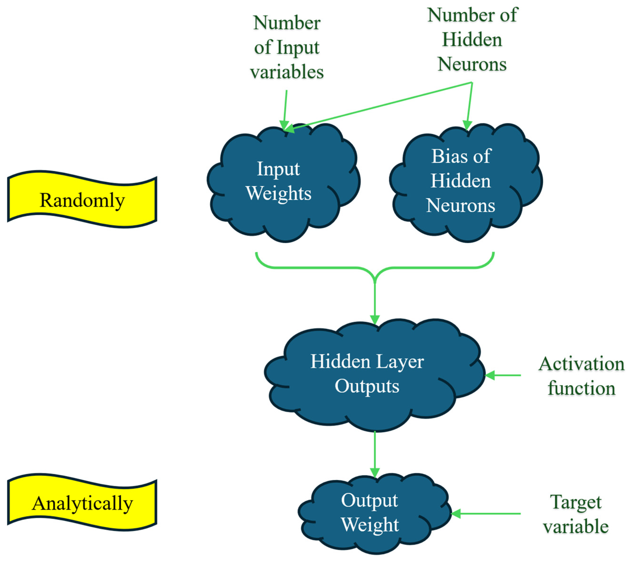
Figure 3.
Flowchart of the developed AELMPSO for feature selection.
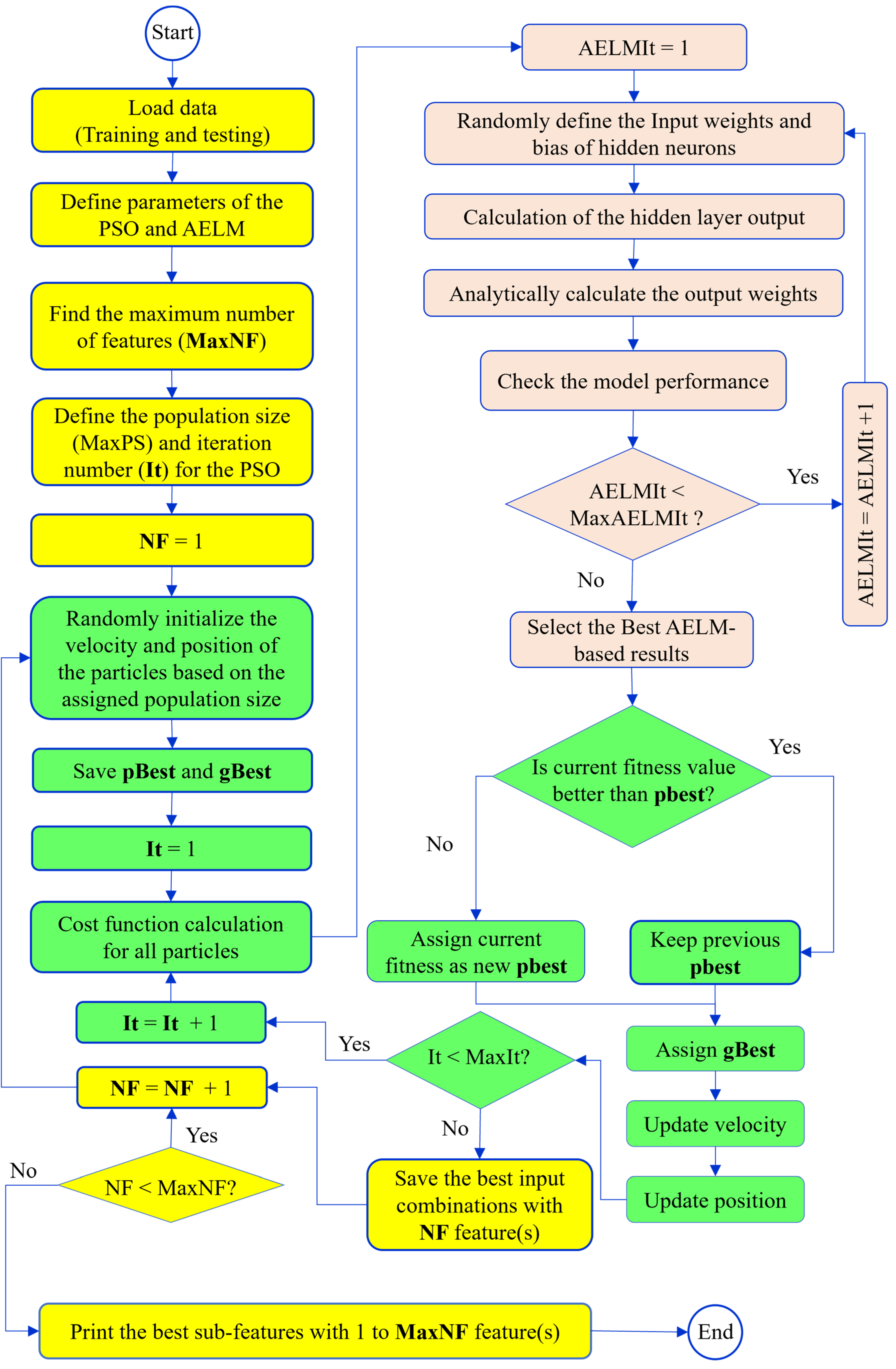
Figure 4.
Results of the feature selection
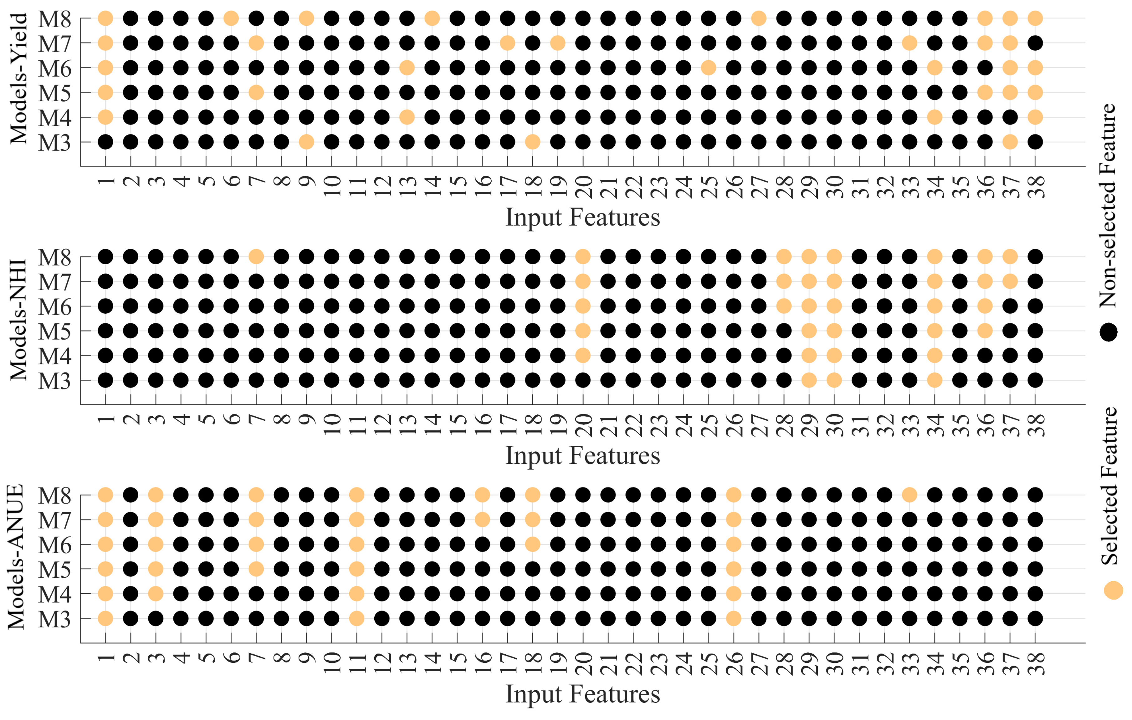
Figure 5.
Performance evaluation of the AELM-based models for predicting Yield (outermost circle), NHI (middle circle), and ANUE (innermost circle) across models with three to eight features. The charts are read counterclockwise, where the segment between two model labels (e.g., M3 and M4) represents the value associated with the first model (M3). The color scale indicates the performance values, with variations from low (blue) to high (red) based on the provided gradient legend.
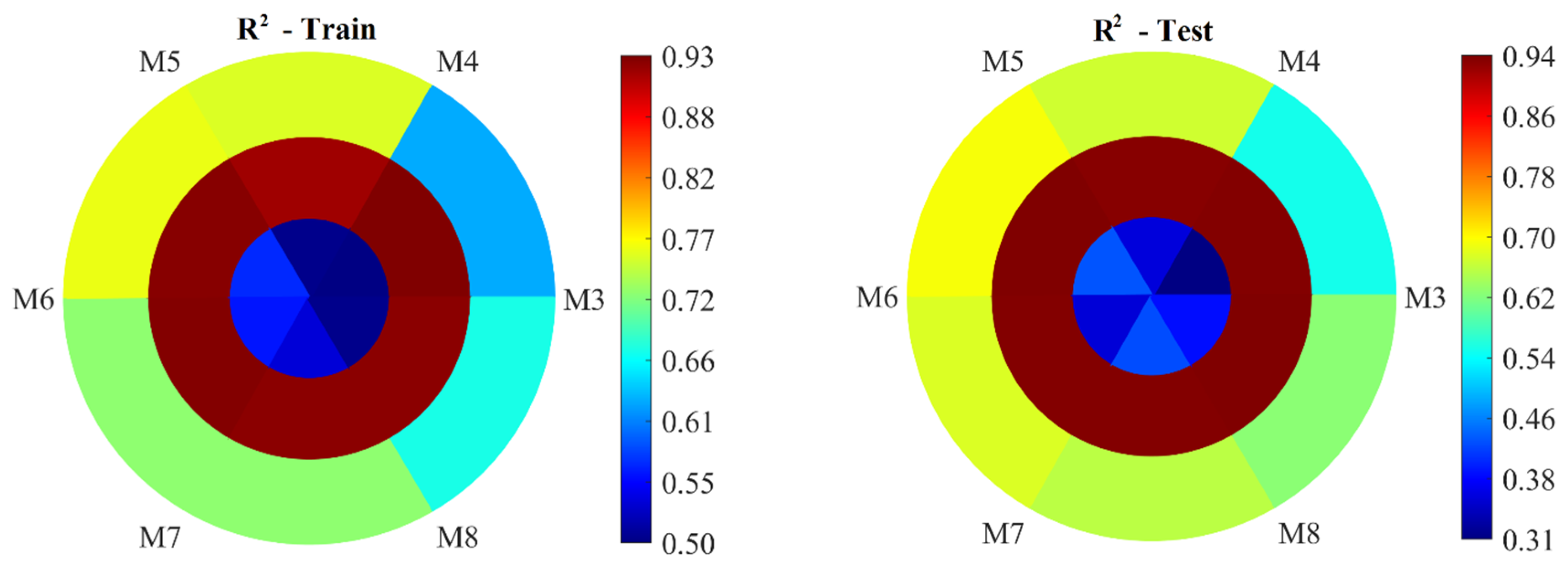
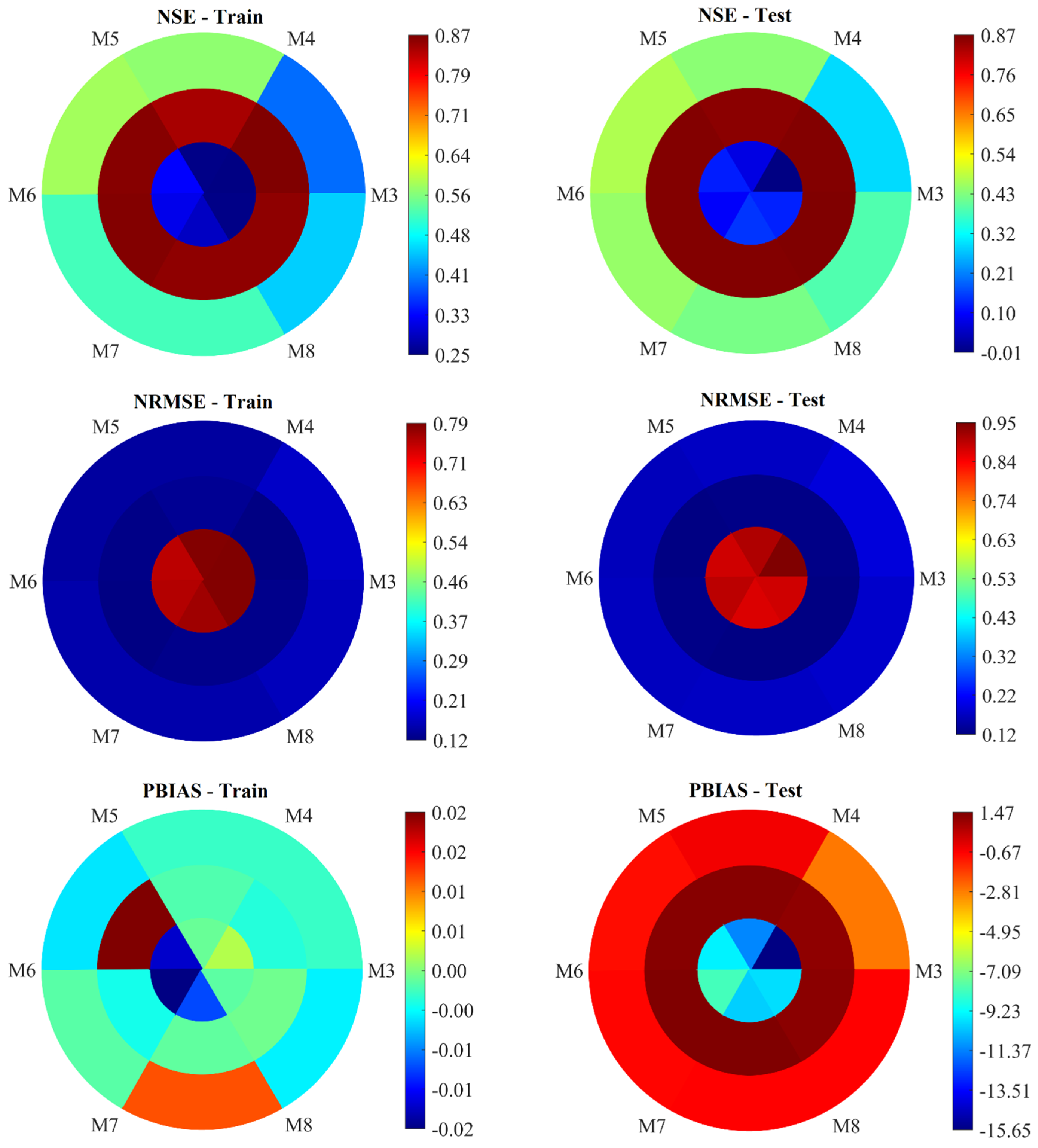
Figure 6.
Relative error across all models in estimating Yield
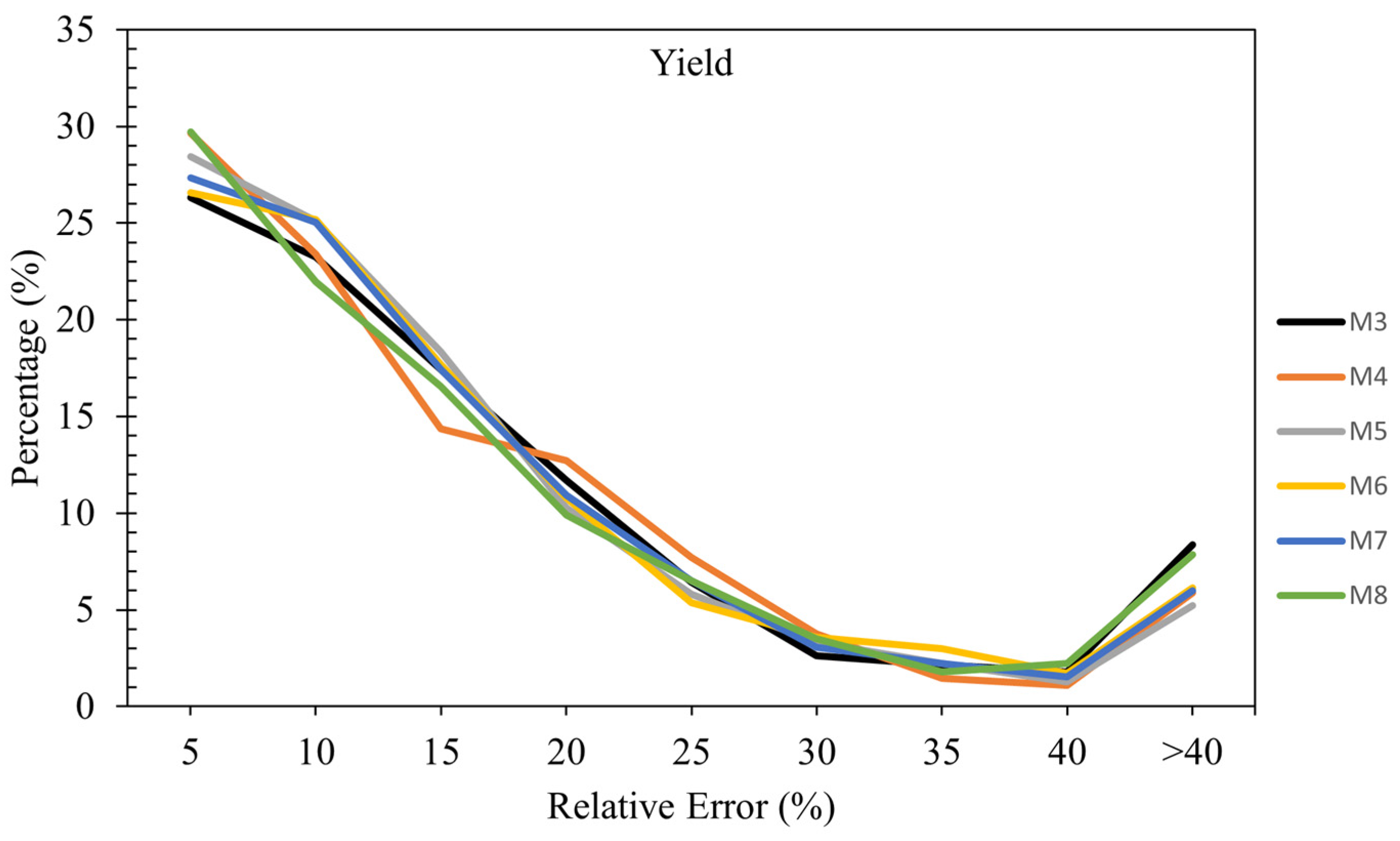
Figure 7.
Relative error across all models in estimating NHI
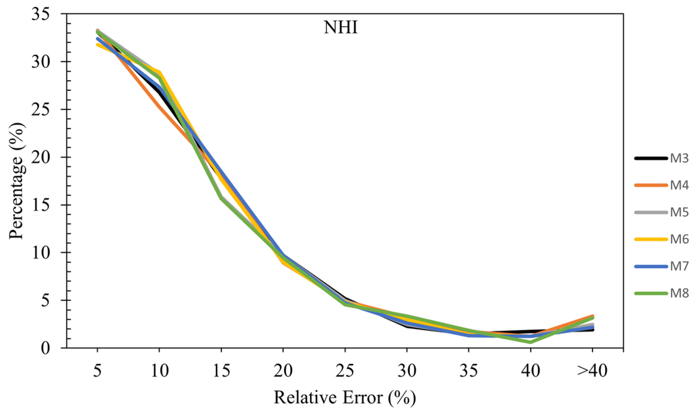
Figure 8.
Relative error across all models in estimating ANUE
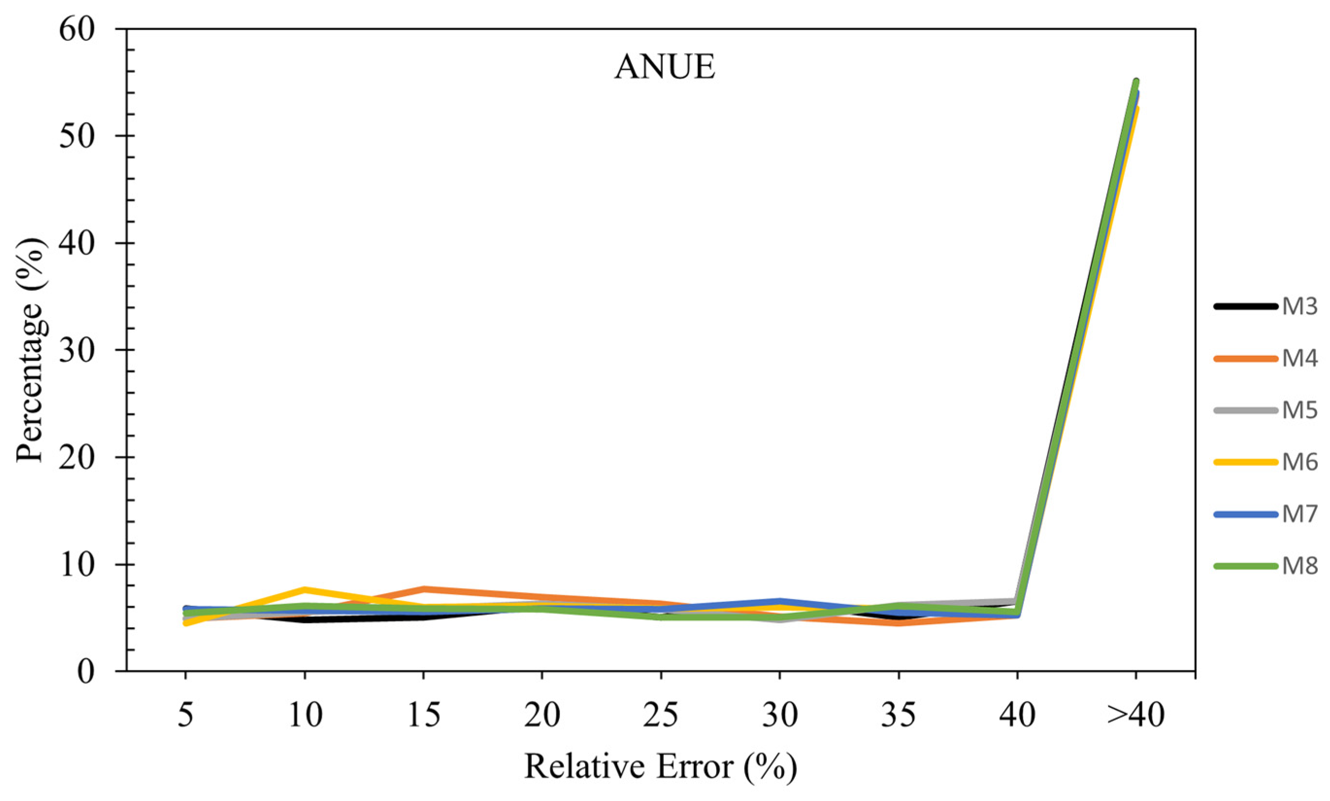

Table 1.
Inputs (1 to 38) and outputs (1 to 3) definitions.
| Variable | Definition | Input / Output No. |
|---|---|---|
| N_Rate | Side dress N rate applied (kg/ha) | In1 |
| Texture | Group of Soil Texture (G1, G2, G3) | In2 |
| Tillage | Type of tillage (Conventional Plowing ; Reduced Tillage ; Direct Drilling) | In3 |
| pH | Soil pH | In4 |
| OrgMat | Organic Matter (%) | In5 |
| P_M3 | P Mehich-3 (kg/ha) | In6 |
| K_M3 | K Mehich-3 (kg/ha) | In7 |
| Ca_M3 | Ca Mehich-3 (kg/ha) | In8 |
| Mg_M3 | Mg Mehich-3 (kg/ha) | In9 |
| Al_M3 | Al Mehich-3 (mg/kg) | In10 |
| Init_NO3 | Initial soil nitrates (mg/kg) | In11 |
| Tassel_NO3 | Soil nitrates at tasseling stage (mg/kg) | In12 |
| Harvest_NO3 | Soil nitrates at harvest (mg/kg) | In13 |
| BD_0_15 | Bulk Density 0-15 cm (g/cm3) | In14 |
| BD_15_30 | Bulk Density 15-30 cm (g/cm3) | In15 |
| BD_30_45 | Bulk Density 30-45 cm (g/cm3) | In16 |
| BG | β-glucosidase enzyme activity at harvest (nmol/g dry soil/h) | In17 |
| Init_BG | β-glucosidase enzyme activity pre-side dress (nmol/g dry soil/h) | In18 |
| NAG | N-acetyl-β-glucosaminidase enzyme activity at harvest (nmol/g dry soil/h) | In19 |
| Init_NAG | N-acetyl-β-glucosaminidase enzyme activity pre-side dress (nmol/g dry soil/h) | In20 |
| FDA | Fluorescein diacetate activity at harvest (µg/h/kg dry soil) | In21 |
| Init_FDA | Fluorescein diacetate activity pre-side dress (µg/h/kg dry soil) | In22 |
| RM | 24 h Microbial respiration at harvest (mg C-CO2/kg dry soil/h) | In23 |
| Init_RM | 24 h Microbial respiration pre-side dress (mg C-CO2/kg dry soil/h) | In24 |
| PRT | ACE Soil Proteins at harvest (g/kg dry soil) | In25 |
| Init_PRT | ACE Soil Proteins pre-side dress (g/kg dry soil) | In26 |
| CHU_May | Accumulated Corn Heat Units (May) | In27 |
| CHU_June | Accumulated Corn Heat Units (June) | In28 |
| CHU_July | Accumulated Corn Heat Units (July) | In29 |
| CHU_August | Accumulated Corn Heat Units (August) | In30 |
| CHU_September | Accumulated Corn Heat Units (September) | In31 |
| CHU_October | Accumulated Corn Heat Units (October) | In32 |
| Rain_May | Accumulated Rain in mm (May) | In33 |
| Rain_June | Accumulated Rain in mm (June) | In34 |
| Rain_July | Accumulated Rain in mm (July) | In35 |
| Rain_August | Accumulated Rain in mm (August) | In36 |
| Rain_September | Accumulated Rain in mm (September) | In37 |
| Rain_October | Accumulated Rain in mm (October) | In38 |
| Yield | Dry Yield (Humidity: 14,5%) (kg/ha) | Out1 |
| NHI | Nitrogen Harvest Index (%) | Out2 |
| ANUE | Agronomic Nitrogen Use Efficiency (kg grain/kg N applied) | Out3 |
Table 2.
Calculation of all possible sub-features for 1 to 38 features.
| No. of inputs | No. of sub-features | No. of inputs | No. of sub-features | No. of inputs | No. of sub-features | No. of inputs | No. of sub-features |
|---|---|---|---|---|---|---|---|
| 1 | 3.90E+01 | 11 | 1.68E+09 | 21 | 6.24E+10 | 31 | 6.15E+07 |
| 2 | 7.41E+02 | 12 | 3.91E+09 | 22 | 5.10E+10 | 32 | 1.54E+07 |
| 3 | 9.14E+03 | 13 | 8.12E+09 | 23 | 3.77E+10 | 33 | 3.26E+06 |
| 4 | 8.23E+04 | 14 | 1.51E+10 | 24 | 2.51E+10 | 34 | 5.76E+05 |
| 5 | 5.76E+05 | 15 | 2.51E+10 | 25 | 1.51E+10 | 35 | 8.23E+04 |
| 6 | 3.26E+06 | 16 | 3.77E+10 | 26 | 8.12E+09 | 36 | 9.14E+03 |
| 7 | 1.54E+07 | 17 | 5.10E+10 | 27 | 3.91E+09 | 37 | 7.41E+02 |
| 8 | 6.15E+07 | 18 | 6.24E+10 | 28 | 1.68E+09 | 38 | 3.90E+01 |
| 9 | 2.12E+08 | 19 | 6.89E+10 | 29 | 6.36E+08 | Sum | 5.50E+11 |
| 10 | 6.36E+08 | 20 | 6.89E+10 | 30 | 2.12E+08 |
Table 3.
Descriptive performance of statistical metrics.
| Index | R2 | NSE | PBIAS | NRMSE | |
|---|---|---|---|---|---|
| Descriptive performance | Unsatisfactory | R2 < 0.5 | NSE < 0.4 | PBIAS > ±25% | 30 % < NRMSE |
| Acceptable | - | 0.4 < NSE < 0.5 | - | - | |
| Satisfactory | 0.5 < R2 < 0.6 | 0.5 < NSE < 0.65 | ±15% > PBIAS > ±25% | 20 % < NRMSE< 30 % | |
| Good | 0.6 < R2 < 0.7 | 0.65 < NSE < 0.75 | ±10% > PBIAS > ±5% | 10 % < NRMSE < 20 % | |
| Very Good | 0.7 < R2 < 1 | 0.75 < NSE < 1 | ±5% > PBIAS | NRMSE < 10 % |
Disclaimer/Publisher’s Note: The statements, opinions and data contained in all publications are solely those of the individual author(s) and contributor(s) and not of MDPI and/or the editor(s). MDPI and/or the editor(s) disclaim responsibility for any injury to people or property resulting from any ideas, methods, instructions or products referred to in the content. |
© 2024 by the authors. Licensee MDPI, Basel, Switzerland. This article is an open access article distributed under the terms and conditions of the Creative Commons Attribution (CC BY) license (http://creativecommons.org/licenses/by/4.0/).
Copyright: This open access article is published under a Creative Commons CC BY 4.0 license, which permit the free download, distribution, and reuse, provided that the author and preprint are cited in any reuse.


