
Submitted:
21 December 2024
Posted:
24 December 2024
You are already at the latest version
Abstract
Disc cutters are essential for shield tunnel construction, and monitoring their wear is vital for safety and efficiency. Due to their position in the soil silo, it is more challenging to observe the wear of disc cutters directly, making accurate and efficient detection a technical challenge. However, the existing detection methods have problems such as higher costs, more difficulty explaining the model, and low prediction accuracy. To solve these problems, this paper proposes a new disc cutter wear state detection method, called multivariate selection attention prototype network(MVSAPNet). The method introduces an attention prototype network for variable selection, which selects important features from many input parameters by a specialized variable selection network. To address the problem of imbalance in the wear data, a prototype network is used to learn the centers of the normal and wear state classes, and the detection of the wear state is achieved by detecting high-dimensional features and comparing their distances to the class centers. The method performs better on the data collected from the Ma Wan Cross-Sea Tunnel project in Shenzhen, China, with an accuracy of 0.9187 and an F1 score of 0.8978, higher than the experimental results of other classification models.
Keywords:
tunnel boring machine
; disc cutter
; deep learning
; interpretability
; time series clasification
1. Introduction
Shield machines, as a kind of tunnel driving equipment with fast speed, small impact on the surroundings, safety, and low cost, have been widely promoted in subways, highways, urban pipe galleries, and other fields in recent years. As the core component of the shield machine, disc cutters are installed on the surface of cutterhead, which use the tangential force brought about by the rotation of disc cutters to crush and cut hard rocks, so disc cutters will gradually wear out with the increase in the distance of advancement. Moreover, the frequency of wear of the cutters and other situations will significantly increase in the hard strata. However, since disc cutters are located in the front of the earth silo, it is difficult to directly observe the overall wear of disc cutters with the naked eye, and frequent opening of the silo to check the delay in the work schedule at the same time will produce a certain amount of safety hazards. There are two ways of judging the overall wear of disc cutters: the direct way and the indirect way. The direct way is through the experience of construction personnel, regular spot checks, or combined with sensors or special materials to assist detection. Although the auxiliary detection method is more accurate in recognizing wear, it has specific cost and equipment limitations [1,2]. The other is the indirect method, which detects blade wear indirectly through the primary propulsion data during shield propulsion.
Existing cutter wear detection methods are mainly categorized into three approaches: mechanism model, energy analysis, and data-driven methods.
The mechanistic approach models the rock fragmentation process through mechanical analysis and maps it to other digging parameters. Wang et al. [3] used the displacement equation of the rock-breaking point on the cutter ring to construct a wear prediction model by combining the theoretical analysis of the cutter force and wear test. She et al. [4] proposed a calibrated expression for the CSM model’s typical load, creating a theoretical model to predict cutter wear during rock breaking and identifying a quantitative link between the wear index and various factors. Yang et al. [5] proposed a cutter wear coefficient and a calculation method based on track weight to accurately calculate the cutter wear under the non-homogeneous stratum based on the cutter wear model proposed by the Japanese Tunneling Association.
Many researchers started from the energy analysis point of view by monitoring the cutter’s temperature change or energy exchange on the disc cutter, which can effectively detect the wear of disc cutters. Wang et al. [6] proposed and calculated the energy conversion coefficient and thrust distribution coefficient to predict disc cutter wear in shield tunneling. Yang et al. [7] proposed a new method to predict the depth of disc cutter wear based on energy analysis according to the geometry of disc cutters and the relationship between the wear loss and the friction work. She et al. [8] further estimated disc cutter wear by analyzing the conversion mechanism between disc cutter wear energy and wear capacity, establishing the relationship between the energy conversion relationship and rock properties.
Many data-driven methods have emerged with the wide application of machine learning and even deep learning methods in the field of machinery fault diagnosis, along with sensor technology innovation. These methods learn wear-related features of disc cutters by utilizing the data collected by the sensors at the shield site, combined with machine learning and deep learning models, and thus finally achieve the detection or prediction of wear. Kim, Y et al. [9] used excavation data collected during shield tunneling to predict the wear of disc cutters using five different machine-learning techniques. Kilic K et al. [10] employed a one-dimensional convolutional neural network (1D-CNN) model to estimate the wear of each cutter in a real-time manner using data collected by soil pressure balance shield during tunneling in soft ground to perform cutter wear prediction. Kim. Y et al. [11] classified the abnormal wear state of disc cutters during shield tunneling by comparing the machine learning classification methods such as KNN, SVM, and DT to assess the need for disc cutter replacement. Zhang N et al. [1] developed a model that integrates a 1D-CNN, a Gated Recurrent Unit Network (GRU) and used a multi-step forward prediction approach to achieve the prediction of tool wear for soil pressure balance shields. Liu Y et al. [2] used a kernel support vector machine (KSVM) to construct a mapping model between disc cutter replacement judgments and established features to determine whether disc cutter replacement is currently required.
However, although the mechanistic analysis method can more accurately predict the amount of disc cutter wear under normal digging conditions, it is often limited to the estimation before digging and the situation during regular digging. In contrast, the energy analysis method can detect abnormal wear. However, it is prone to be interfered with by other abnormal events, which reduces identification accuracy. The field data-driven method can overcome the above shortcomings simultaneously, so more and more scholars are gradually adopting the data-driven method to detect disc cutter wear. Most of the existing data-driven methods predict the wear of each cutter, rely on specific geological parameters, or can only realize the prediction of normal advancement wear of disc cutters. In the tunneling process, there is no need to monitor each tool’s status, and the cutter’s overall cutting performance is more important than the specific wear value of a single cutter. [2] Therefore, detecting and determining whether the current cutter needs to be opened and replaced is more practical. In addition, composite strata are usually composed of many different soil and rock types, such as sand, clay, gravel, soft rock, and hard rock. These strata have pretty different physical and mechanical properties, and their distribution and thickness change more frequently, resulting in the continuous adjustment of the parameters to adapt to the shield machine’s different geologic conditions in tunneling, making disc cutters more prone to abnormal wear and tear of disc cutters. Therefore, detecting wear state of disc cutters in the composite strata is more complex than in single homogeneous strata. [12]
Based on the above-mentioned problems, this paper proposes a multivariate selection attention prototype network(MVSAPNet) driven by sensor data collected during the shield tunneling process, which detects cutter head wear state by comparing the distance of time-dependent features to the center of each class. The specific contributions of this paper are as follows: (1) A new prototype network for variable selection is proposed to classify unbalanced disc cutter wear data, and the proposed model is more effective than other classification models in detecting the data scenarios of the Ma Wan Cross-Sea Tunnel project. (2) Multiple preprocessing methods are used to extract the relevant features of the data to ensure that the model performs well on the disc cutter wear state detection task in composite strata. (3) By obtaining the intermediate parameters and interclass distance of the model, it was found that real-time parameters such as cutter speed, penetration, FPI, and TPI change significantly when the disc cutter wear occurs. This verifies the accuracy of the long-term experience accumulated by the actual constructors and provides a practical research idea for predicting disc cutter wear.
2. Materials and Methods
Based on the above existing problems, the overall framework of the disc cutter wear detection proposed in this paper is shown in Figure 1. It is mainly composed of 4 parts. First of all, for the raw data extracted from the database, due to the existence of a large number of data in the assembling stage which is not related to the wear process, it is necessary to extract the data in the advanced state and then reconstruct the data to remove the outliers through the LSTM-ED algorithm [13], and denoise the data with the VMD-WT algorithm. After that, the data features are initially extracted by feature engineering using a specific method and then split datasets. Finally, the data is trained using the classification detection model proposed in this paper to classify the disc cutter’s state.
2.1. Preprocessing
The acquired shield operation data needs a series of preprocessing operations to make the original data from sensors easier to train. Figure 2. shows the specific process. First of all, shield tunneling is divided into the propulsion state and the assembling state. However, the disc cutter almost only wears out in the propulsion state, so it is necessary to extract the shield propulsion state data from the database. For the acquired propulsion state data, the Z-Score method is used with the following formula:
where denotes the data of the parameter at the moment t, denotes the mean value, denotes the standard deviation and N denotes the number of selected sensor data.
In addition, due to a variety of disturbing factors and abnormalities in the shield tunneling process, there are often a variety of abnormal outliers in raw data, so it is necessary to detect and eliminate the outliers. Commonly used outlier detection methods include the mean square deviation, box plot, clustering, reconstruction, and others. Autoencoder(AE) is an unsupervised learning method for data reconstruction and feature learning to achieve dimensionality reduction or anomaly detection. It mainly consists of two parts, an encoder and a decoder, which are responsible for compressing data into the latent space and reconstructing data from that space. The autoencoder can reconstruct normal data correctly by learning the feature patterns in normal data. However, it has a limited effect on handling outliers so that it can be used for anomaly detection. Meanwhile, since LSTM can extract feature information from time series, it can better capture long-term dependencies in time series compared to CNN architecture, and it can also solve the problems of gradient vanishing and gradient explosion encountered by traditional RNN when dealing with long sequence data, so it is more suitable for coding shielded time-series data. In this paper, we decided to use the LSTM-ED model [13] to remove outliers in the original data. In addition, the LSTM-ED model is optimized by using the inverse-order reconstruction and teacher-forcing strategies, thus avoiding the accumulation of errors in the model to a certain extent and further improving the reconstruction ability of the model. The average absolute error is used as the reconstruction error of the model with the following formula:
For the reconstruction error, the outliner is defined by applying the criterion, and the threshold is set as follows:
where denotes the filter threshold, and denote reconstruction mean and standard deviation error. For the average reconstruction error at each time step corresponding to different sliding windows, the threshold is used to determine if it is an outlier, discard it, and fill it by interpolation.
Although the LSTM-ED method can remove the anomalous data collected by shield sensors that are inconsistent with the global distribution as well as some of the high-frequency noises, the data collected during shield tunneling are subject to various interferences from the equipment sensors themselves, the stratum, and the personnel’s operation. The effect of reducing the impact of the noise is limited only by the reconstruction method. Therefore, it is necessary to denoise the data further. The main idea of the Variational Modal Decomposition (VMD) [14] is to decompose the signal into multiple intrinsic modal functions (IMFs) and a residual component, where different IMFs represent different frequency components of the signal, and the residual is the remaining portion of the original signal. Unlike the Empirical Mode Decomposition (EMD) method, VMD overcomes the endpoint effect and modal aliasing problems of EMD by adaptively matching each mode’s optimal center frequency and finite bandwidth, which can reduce the non-stationary time series with high complexity and nonlinearity, and widely used in different engineering fields. [15,16,17] Therefore, this paper uses VMD combined with WT to denoise and filter the shield data. Using VMD, the shield parameters are decomposed into seven different IMFs, denoted as IMF1-IMF7, where IMF7 has the highest center frequency. For IMF4-IMF6, due to the presence of a certain level of noise, each component is denoised by using the WT wavelet transform. Set sym4 as the wavelet base, and the noise is denoised using empirical Bayes combined with a posterior mean threshold. As for IMF1-IMF3, they are kept unchanged due to their lower frequencies, which represent the characteristics of the original signal. Finally, summing up IMF1-IMF3 and the denoised IMF4-IMF6 to regain the denoised signal.
For the denoised shield data, features can be initially extracted using feature engineering to enhance the input to the model. Since the shield machine sensors collect data at a low frequency, generally in seconds or minutes, or in millimeter travel (mm), it is not suitable to analyze the shield timing data from a frequency domain perspective, as this will produce a more serious aliasing problem. Therefore, the shield data is often analyzed by constructing time-domain features. Combined with the features used in other studies [18,19,20], the features selected in this paper are shown in Table 1.
However, when more parameters are selected, the time-domain feature extraction will make a large input dimension, which can produce a dimensional disaster. It can introduce noise to lead to overfitting easily, deteriorate the detection effect of the generalization, and at the same time increase the complexity of computation and training difficulty of the model, so it is necessary to introduce some index to the input features to reduce the dimensionality of the model. Since disc cutter wear is irreversible, the input features should have a certain degree of monotonicity and trend for a complete blade wear process [21,22]. These metrics can be calculated respectively:
where denotes the data at time t, N denotes number of data, denotes step function. After calculating all the data monotonicity and trend metrics, each metric is normalized and then summed to get the final score and obtain the features with the top 50 scores as model inputs for training.
2.2. Multivariate Selection Attention Prototype Network
After selecting the appropriate features as model inputs, the next step is training using the Multivariate Selected Prototype Classification Network (MVSAPNet) proposed in this paper. Figure 3. shows the overall structure of the model, which consists of three parts: the Variable Selection Network (VSN), Temporal Processing, and Class Prototype Learning.
2.2.1. Variable Selection Network (VSN)
The operating parameters during shield propulsion are affected by various aspects, such as the stratum and the parameters of the tunnel shield itself, and these parameters may have a positive effect on the overall training of the model. Inspired by Bryam Lim et al. [23], we introduce gated residual network (GRN) to promote the extracted features to better non-linearly fuse with the auxiliary feature parameters, whose overall structure is shown in Figure 3. GRN accepts a primary feature and an optional auxiliary context feature as inputs, after which two linear layers realize the initial fusion of the two features, and an exponential linear unit activation function (ELU) [24] is used between the linear layers to enhance the fitting ability between the inputs. The results are input into gated linear units (GLUs) after a dropout layer, prompting the GRN to be able to control the degree of contribution of the input feature sequences. Finally, superimposition with the main features using residual concatenation makes it possible to increase the speed of model training while enhancing the model’s fitting ability:
where i denotes the primary feature of input, e denotes optional auxiliary context feature, denotes the sigmoid activation function, W and b are weights and bias.
For many input features, conventional classification algorithms find it difficult to accurately measure the specific contribution of different variables to the output. The effectiveness of the model is often measured by comparing the features in the middle, which is not a good way to show the contribution of different input features to the whole model. Therefore, the feature variable selection network (VSN) is introduced as the first part of the model. For a set of input feature sequences, the VSN first encodes each dimension of the input feature data, and the encoding dimension is set to 128, which can amplify the input features and thus represent the more profound information of the sequences, facilitating the subsequent extraction and classification of features. After that, the data for each timestamp is set into the GRN network, and the data for all timestamps is inputted to GRN after flattening. The corresponding selection weights of each variable are obtained through softmax. Finally, the feature output is superimposed. The purpose of introducing VSN in this way is not only to be able to realize the selection of input variables but also to be able to control the degree of contribution to a certain extent by deleting the input or noise that does not contribute much to the classification model, so the variable selection network can better help the model to improve the classification performance.
2.2.2. Temporal Processing
Due to the characteristics of time series collected in tunnel machines, there is no point in observing the data at a particular timestamp alone for judgment. The significance of time series data lies in comparing with other timestamps in the context, and thus modeling temporal dependencies is crucial in various time series tasks. Compared to CNNs, which focus more on local patterns, LSTMs use four gates with different effects to focus more on long-term patterns in the data while retaining short-term information. They are more suitable for modeling long-term dependence features of time series. Therefore, we use an LSTM-Encoder structure to learn the temporal dependencies of shielded feature data. After the LSTM-Encoder for each time step input, a corresponding latent layer output is obtained and finally outputs the features through a gated network and a residual structure.
2.2.3. Class Prototype Learning
Since the data on disc cutter wear have characteristics of specific data imbalance and the wear samples are severely limited, it is difficult for conventional classification and detection algorithms to train the model and learn practical fault features directly. Inspired by TapNet [25], we introduce the attention prototype model in the training process to train different class feature prototypes for different classes in the training process and realize the detection of blade wear state by comparing the distance between the test data features and each class prototype. Figure 5 shows the overall structure of the attention prototype model. First, for the input features, a mapping layer consisting of two fully connected layers is used for dimensionality reduction. Assuming that the input features are , where L is the length of the sliding window and E is the embedding of series data:
where denotes spreading operation, W, b are weight and bias, is batch normalization and is activation function.
After that, the dimensionality-reduced data are input into an attention pool for training according to labels. Different training labels correspond to different attention models in the attention pool, so the number of classes corresponds to the number of attention models in the attention pool. After training, obtain an attention score:
where denotes the weight of i sample belonging to k class, denotes the embeddings of input data, and are weights of attention model, which u is an settable hyperparameter. Then, multiply the feature data and the attention score to produce the class vector.
After training, each class has a corresponding class prototype vector, and the vectors are spliced to get a class prototype matrix. In the test phase, the latent features are obtained by the Mapping Layer and the class prototype matrix of each class to calculate the distance. The distance can be calculated by Euclidean distance, the Mahalanobis distance and others. In this paper, we use Euclidean distance to calculate the distance. Moreover, because of the probability value obtained from the classification is based on the similarity of the distance between the class prototype vector and the feature vector, the smaller the distance should get the higher the similarity. Hence, we need to invert the result of the distance function.
where D denotes the Euclidean distance. Finally, the training is optimized using Adam’s algorithm to minimize the negative logarithmic probability loss.
3. Results
3.1. Engineering Background
The raw data used in this paper are from the shield advancement data of the Ma Wan Cross-Sea Tunnel project in Shenzhen, China, during the period from 13:32 on August 9, 2022, to 0:48 on October 11, 2022, using the Herrenknecht large-diameter slurry pressure balance shield, and passing through the geological conditions of the upper-soft and lower-hard composite strata (upper fully-weathered mixed granite, middle earth/massive strongly weathered granite, lower slightly-weathered mixed granite) transitioning to hard-rock strata (slightly-weathered mixed granite). Since the shield propulsion is carried out in rings, there is a long stopping period between rings for assembling the pipe pieces and the digging process takes up only a tiny part of the time. The wear process occurs almost exclusively during the digging when the disc cutter is rotating. It is necessary to extract the data in the digging working condition during this period for analysis. After extraction, 393,887 working state data were collected from the database. Due to the performance and failure of the sensor itself, there are some duplicated and missing data for the acquirement. Hence, the data needs to be de-duplicated and interpolated. After that, the data are sampled with a sampling interval of 20s, and 55,932 sequence data are obtained after processing. Based on the previous work and the observation of the actual sensor data available in the tunnel, 15 parameters are selected for analysis, and the details are listed in Table 2. Penetration indicates the distance advanced by rotation of the disc cutter and is used to reflect the overall cutting capacity of the disc, which is defined by . v is mean excavation speed and f is cutterhead speed. FPI reflects the positive force required during cutter boring, which is defined by . F denotes total thrust. TPI reflects the tangential force required during cutter boring, which is defined by . T denotes cutterhead torque.
3.2. Data Preprocessing
After that, the input data are normalized and divided into small sub-windows for reconstruction using a sliding window of length 15 and step size 1, resulting in a total of 55,917 windows. All the windows were input into the LSTM-ED model for training, where the LSTM hidden layer parameter was set to 64, and the number of layers was set to 1. The model was also optimized using the inverse-order reconstruction and teacher-forcing strategies. The cutterhead speed reconstruction results are shown in Figure 4. using the Adam optimizer training and setting the learning rate to 0.001.
It can be seen that after filtering, the results appear significantly smoother, effectively addressing outliers and mitigating the impact of noise to a certain extent. Next step, the data are denoised by VMD-WT transform. This paper decomposes the shield parameters into 7 different IMFs, denoted as IMF1-IMF7, and setting the penalty term to 2000, where IMF7 has the highest center frequency. For IMF7 and the residuals of VMD decomposition can be eliminated due to the high-frequency noise and little contribution to the whole time series. Figure 6 shows the comparison results with cutterhead speed.
Finally, time-domain features are extracted separately for each parameter through sliding windows which set window length as 10 and step size as 3. After feature extraction, 165 primary features were obtained. Table 3 shows result of calculating trend and monotonicity scores for features. After that, the features with Top 50th scores are selected as model inputs for training.
Since this paper adopts various methods to preprocess the shield acquisition data, to assess better the impact of each step in the preprocessing on the results, test the data obtained from each step in preprocessing is output separately with the model proposed by the paper. Figure 6. shows the final experimental results, where the results of each step are obtained based on the previous step. It can be seen that compared to the initial feature selection achieved without preprocessing the data, the training effect of the data after preliminary processing is improved by about 14%, which may be due to the limited wear data samples that can be used for training, and it is challenging to train the data directly to obtain more generalized disc cutter wear features. In addition, it can be noted that compared with selecting all features, only using the top 50 features for training can still improve performance by about 2%. On the one hand, features other than the top 50 may impact the disc cutter wear detection effect less. On the other hand, too high dimensional data will reduce the computational efficiency while leading to dimensionality explosion, thus affecting the model’s overall performance.
3.3. Comparison Models
After preprocessing, 18668 trainable data were finally obtained. Considering the change in data distribution due to the gradual transition of the tunnel cut from the upper soft and lower hard strata to the hard rock strata during the acquisition of data for the segment, a total of 7348 pieces of data from one section of a complete upper soft and lower hard stratum and another section of a complete hard rock stratum were used as the training set, and the remaining 11320 pieces of data were used as the test set for inspection. Six disc cutter wear events occurred in the shield and two in the selected training data. For the classification detection model hyperparameters, the learning rate LR is set to 0.0001, the batch size is set to 64, the number of iterations is 200, the sliding window length is 20, the LSTM output layer size is 128, the dropout layer is 0.2, the attention dimension is set to 64, the gradient clipping is set to 0.2, the loss function adopts the cross-entropy loss function, and train with Adam optimizer.
The most commonly used metrics for the evaluation metrics of classification results are the accuracy and the f1-score. For shield data, since the disc cutter wear abnormality accounts for a small percentage of the overall dataset and the overall dataset is unbalanced, the f1-score is more reflective of the detection results, so we takes the f1-score as the main evaluation index of the model.
In order to show the advantages of the proposed model, we use important or newer deep learning models in the field of time series classification to compare, including (1) Recurrent-based networks: LSTM-FCN, ALSTM-FCN [26] and BiLSTM. (2) Kernel-based networks: ResNet, InceptionTime [27]. (3) Transformer-based networks: GTN [28], TARNet. (4) Other types of networks: TapNet [25]. Table 4 shows the experimental results.
The results show that our proposed model performs better on the shield disc cutter wear dataset compared to several important baseline methods, with an accuracy of 0.9187 and an F1 score of 0.8978, higher than the experimental results of the other compared models. ALSTM-FCN works better compared to BiLSTM, probably because ALSTM-FCN employs an attentional approach to learn the importance of the input features of the shield data, which is more important than learning the bi-directional dependencies of the shield data. It is also found that the recurrent neural network is close to or even exceeds the relatively more complex kernel model on the shield disc cutter wear dataset. Maybe disc cutter wear data are more affected by time-dependent features in the long term, whereas kernel models are more concerned with numerical or shape-based features. Based on these points, it is expected that the transfomer-based network model outperforms the recurrent and kernel models, and the actual results align with this speculation. However, the transfomer-based model must be trained on a large amount of data to learn sufficient data features. Obtaining a large amount of wear data for the disc cutter wear is challenging. This data imbalance weakens the performance of transfomer-based model. Therefore, it can be seen that TapNet, which also employs a prototype-like network, is able to approach Transfomer’s model in terms of real-world detection results. The proposed model MVSAPNet, which introduces a variable selection network to strengthen the feature selection ability of the model, absorbs the ability of the recurrent neural network to learn the time-dependent characteristics and adopts the Prototype mechanism better to overcome the characteristics of the shield data imbalance, so it produces a better detection effect on the disc cutter wear dataset.
In order to prove the effectiveness of each part of the proposed model for the whole network, ablation experiments are required, the results of which are shown in Figure 7. The GRN and VSN modules are directly removed, and the front and back inputs and outputs are directly connected. A fully connected layer replaces the Prototype module. The results show that GRN can better enhance the nonlinear ability of the model to learn the features of disc cutter wear better; VSN can very effectively improve the detection effect of the model while selecting the variables through different weights and improve the interpretability of the disc wear anomalies to a certain extent by obtaining the selected weights. The prototype network can improve the model’s ability to detect disc cutter wear to a certain extent by using the attention mechanism to extract key features and the normal state as class prototype vectors and calculating the distance between the current state and the prototype vectors of shield for detection.
4. Discussion
To more accurately assess which shield parameters are more correlated with the overall level of disc cutter wear, we trained all features and visualized the selection weights in the variable selection module VSN, and the results are shown in Figure 8. In this figure, the horizontal axis represents the selected features. In contrast, the vertical axis represents the different sensor data captured by the shield, and the shade of the color is used to indicate the magnitude of the weights. The weights show that the variable selection network gives relatively large weights to the four parameters of TPI, FPI, penetration, and disc cutter speed in composite strata. It indicates that when the overall disc cutter wear reaches a certain level that affects the cutting efficiency and the cutter needs to be replaced, four parameters of penetration, FPI, TPI, and cutterhead speed change significantly. The weights of the other parameters are relatively small, particularly the cutterhead torque, which means the composite indicator parameters are more suitable for describing the shield state characteristics under different digging conditions than the single sensor parameters, reflecting the fact that a comprehensive judgment of the parameters is needed to judge the disc cutter wear, which is also the reason why evaluation indicators such as TPI, FPI, penetration, are proposed to be used for detecting the disc cutter wear in other works. In addition, it was also found that the excavation speed in the Ma Wan Cross-sea Tunnel did not significantly impact the overall disc cutter wear. Actually, the data showed that the thrust in the sub-zones increased significantly when the disc cutter wear occurred. It is due to increasing the thrust on site to ensure excavation speed despite the disc cutter wear during construction. This finding is consistent with the summaries of experience and feedback reports from the engineers and technicians accumulated during the actual project.
In order to better visualize the relationship between individual samples in the model and the class prototype matrix, t-SNE was employed to project the class prototypes and the samples from both the training and testing phases. Figure 9. shows the results. In figure, the orange points indicate the data of the disc cutter wear state, the blue points indicate the data of the normal state, and the black and red stars represent the centers of the class prototypes of the disc cutter wear state and the normal state. It can be seen that the distribution of the data features of the disc cutter wear state and the normal state has apparent differentiation. However, due to the complexity of the shield tunneling process, human factors, mechanical factors, and stratigraphic factors in the shield tunneling process, the distribution of the data will be shifted with the tunneling process. A small amount of disc cutter wear data has features similar to those of the normal state, which makes some points hard to accurately categorize.
Calculated the difference between the latent vectors and the different classes of vectors in the prototype matrix by the L2-norm to assess the changes in distances between the data features and the vectors of different classes during the advancement. Figure 10. shows the detection results of one of the cases in which disc cutter wear occurs. It can be found that when the shield’s working state is changed except for disc cutter wear, the distance between the shield and the different classes of prototypes will change simultaneously. In contrast, the distance relationship will change when the disc cutter wear occurs. By calculating the difference between the wear distance and normal distance, it can be more clearly seen that under normal propulsion, the difference is roughly stable even under different working conditions. However, when the cutting capacity of the disc cutter decreases, it means that the disc cutter needs to be changed. This difference will drop significantly and eventually reach a negative value, and eventually trigger an alarm. This can prove the model’s effectiveness in detecting disc cutter wear anomalies. At the same time, it provides a new idea for predicting disc cutter wear.
5. Conclusions
In this study, a new prototype network of variable-selective LSTM encoders is proposed to detect the overall wear state of the cutter disc. To better extract the data features, the main parameters related to the cutter wear are selected from the historical excavation data of the Ma Wan Cross-Sea Tunnel. The features of the model are further extracted based on the objective law of wear after denoising the data by LSTM-ED and VMD-WT as the input data of the model. Then a prototype network of variable selection attention prototype model is designed to realize the interpretability of features and results while detecting the state of disc cutter wear. Compared with the existing classification model, the proposed model was superior and can achieve an accuracy of 0.9178 and an f1 score of 0.8978, indicating the model’s effectiveness in the process of shield cutter wear detection and helping to further enhance the effectiveness of the model in the process of shield cutter wear detection and further prediction. However, the model’s generalization needs to be further verified due to the difficulty in obtaining the actual stratum data and the wear amount in the tunnel boring process. In addition, we can incorporate the parameters of the shield machine itself and the stratum parameters as static covariates into the network to achieve a more generalized detection of the overall disc cutter wear state based on the proposed model.
Author Contributions
Data curation, Y.X.; Formal analysis, Y.X. and X.G.; Investigation, Y.X. and X.G.; Methodology, Y.X.; Project administration, X.G.; Resources, X.G. and M.H.; Software, Y.X. and D.h.Y.; Supervision, X.G.; Validation, Y.X. and D.Y.; Visualization, Y.X.; Writing—original draft, Y.X. All authors have read and agreed to the published version of the manuscript.
Funding
This research received no external funding.
Data Availability Statement
The data in the case study are not publicly available due to the confidentiality requirement of the project.
Conflicts of Interest
The authors declare no conflict of interest.
References
- Zhang, N.; Shen, S.L.; Zhou, A. A new index for cutter life evaluation and ensemble model for prediction of cutter wear. Tunnelling and Underground Space Technology 2023, 131, 104830. [Google Scholar] [CrossRef]
- Liu, Y.; Huang, S.; Wang, D.; Zhu, G.; Zhang, D. Prediction Model of Tunnel Boring Machine Disc Cutter Replacement Using Kernel Support Vector Machine. Applied Sciences 2022, 12. [Google Scholar] [CrossRef]
- Wang, Z.; Liu, C.; Jiang, Y.; Dong, L.; Wang, S. Study on Wear Prediction of Shield Disc Cutter in Hard Rock and Its Application. KSCE Journal of Civil Engineering 2022, 26, 1439–1450. [Google Scholar] [CrossRef]
- She, L.; Zhang, S.r.; Wang, C.; Wu, Z.q.; Yu, L.c.; Wang, L.x. Prediction model for disc cutter wear during hard rock breaking based on plastic removal abrasiveness mechanism. Bulletin of Engineering Geology and the Environment 2022, 81, 432. [Google Scholar] [CrossRef]
- Yang, Z.; Sun, Z.; Fang, K.; Jiang, Y.; Gao, H.; Bai, Z. Cutting tool wear model for tunnel boring machine tunneling in heterogeneous grounds. Bulletin of Engineering Geology and the Environment 2021, 80, 5709–5723. [Google Scholar] [CrossRef]
- Wang, X.; Li, S.; Yuan, C.; Ma, P.; Han, Y.; Peng, K. Experimental study on the wear and temperature of TBM disc cutter under different tunneling parameters. Tunnelling and Underground Space Technology 2024. [Google Scholar] [CrossRef]
- Yang, H.; Liu, B.; Wang, Y.; Li, C. Prediction Model for Normal and Flat Wear of Disc Cutters during TBM Tunneling Process. International Journal of Geomechanics 2021, 21, 06021002. [Google Scholar] [CrossRef]
- She, L.; Zhang, S.; Wang, C.; long Li, Y.; Du, M.M. A new method for wear estimation of TBM disc cutter based on energy analysis. Tunnelling and Underground Space Technology 2023. [Google Scholar] [CrossRef]
- Kim, Y.; Hong, J.; Shin, J.; Kim, B. Shield TBM disc cutter replacement and wear rate prediction using machine learning techniques. Geomechanics and Engineering 2022, 29, 249–258. [Google Scholar] [CrossRef]
- Kilic, K.; Toriya, H.; Kosugi, Y.; Adachi, T.; Kawamura, Y. One-Dimensional Convolutional Neural Network for Pipe Jacking EPB TBM Cutter Wear Prediction. Applied Sciences 2022, 12. [Google Scholar] [CrossRef]
- Kim, Y.; Shin, J.; Kim, B. Analysis of disc cutter replacement based on wear patterns using artificial intelligence classification models. GEOMECHANICS AND ENGINEERING 2024, 38, 633–645. [Google Scholar] [CrossRef]
- Ling, X.; Kong, X.; Tang, L.; Cong, S.; Tang, W. Preliminary identification of potential failure modes of a disc cutter in soil-rock compound strata: Interaction analysis and case verification. Engineering Failure Analysis 2022, 131, 105907. [Google Scholar] [CrossRef]
- Srivastava, N.; Mansimov, E.; Salakhutdinov, R. Unsupervised learning of video representations using LSTMs. In Proceedings of the Proceedings of the 32nd International Conference on International Conference on Machine Learning - Volume 37.; pp. 201515843–852.
- Dragomiretskiy, K.; Zosso, D. Variational Mode Decomposition. IEEE Transactions on Signal Processing 2014, 62, 531–544. [Google Scholar] [CrossRef]
- Shi, G.; Qin, C.; Tao, J.; Liu, C. A VMD-EWT-LSTM-based multi-step prediction approach for shield tunneling machine cutterhead torque. KNOWLEDGE-BASED SYSTEMS 2021, 228. [Google Scholar] [CrossRef]
- Zhang, Z.; Li, K.; Guo, H.; Liang, X. Combined prediction model of joint opening-closing deformation of immersed tube tunnel based on SSA optimized VMD, SVR and GRU. OCEAN ENGINEERING 2024, 305. [Google Scholar] [CrossRef]
- Qin, C.; Huang, G.; Yu, H.; Zhang, Z.; Tao, J.; Liu, C. Adaptive VMD and multi-stage stabilized transformer-based long-distance forecasting for multiple shield machine tunneling parameters. AUTOMATION IN CONSTRUCTION 2024, 165. [Google Scholar] [CrossRef]
- Huang, Z.; Zhu, J.; Lei, J.; Li, X.; Tian, F. Tool wear predicting based on multi-domain feature fusion by deep convolutional neural network in milling operations. Journal of Intelligent Manufacturing 2020, 31, 953–966. [Google Scholar] [CrossRef]
- Wu, J.; Wu, C.; Cao, S.; Or, S.W.; Deng, C.; Shao, X. Degradation Data-Driven Time-To-Failure Prognostics Approach for Rolling Element Bearings in Electrical Machines. IEEE Transactions on Industrial Electronics 2019, 66, 529–539. [Google Scholar] [CrossRef]
- Qin, C.; Wu, R.; Huang, G.; Tao, J.; Liu, C. A novel LSTM-autoencoder and enhanced transformer-based detection method for shield machine cutterhead clogging. SCIENCE CHINA-TECHNOLOGICAL SCIENCES 2023, 66, 512–527. [Google Scholar] [CrossRef]
- Guo, L.; Lei, Y.; Li, N.; Yan, T.; Li, N. Machinery health indicator construction based on convolutional neural networks considering trend burr. Neurocomputing 2018, 292, 142–150. [Google Scholar] [CrossRef]
- Javed, K.; Gouriveau, R.; Zerhouni, N.; Nectoux, P. Enabling Health Monitoring Approach Based on Vibration Data for Accurate Prognostics. IEEE Transactions on Industrial Electronics 2015, 62, 647–656. [Google Scholar] [CrossRef]
- Lim, B.; Arık, S.Ö.; Loeff, N.; Pfister, T. Temporal Fusion Transformers for interpretable multi-horizon time series forecasting. International Journal of Forecasting 2021, 37, 1748–1764. [Google Scholar] [CrossRef]
- Clevert, D.A.; Unterthiner, T.; Hochreiter, S. Fast and Accurate Deep Network Learning by Exponential Linear Units (ELUs). arXiv: Learning, 2015. [Google Scholar]
- Zhang, X.; Gao, Y.; Lin, J.; Lu, C.T. TapNet: Multivariate Time Series Classification with Attentional Prototypical Network. In Proceedings of the AAAI Conference on Artificial Intelligence; 2020. [Google Scholar]
- Karim, F.; Majumdar, S.; Darabi, H.; Chen, S. LSTM Fully Convolutional Networks for Time Series Classification. IEEE Access 2018, 6, 1662–1669. [Google Scholar] [CrossRef]
- Ismail Fawaz, H.; Lucas, B.; Forestier, G.; Pelletier, C.; Schmidt, D.F.; Weber, J.; Webb, G.I.; Idoumghar, L.; Muller, P.A.; Petitjean, F. InceptionTime: Finding AlexNet for time series classification. Data Mining and Knowledge Discovery 2020, 34, 1936–1962. [Google Scholar] [CrossRef]
- Liu, M.; Ren, S.; Ma, S.; Jiao, J.; Chen, Y.; Wang, Z.; Song, W. Gated Transformer Networks for Multivariate Time Series Classification. CoRR 2021, abs/2103.14438, [2103.14438]. [Google Scholar]
Figure 1.
The overall framework of the disc cutter wear detection.
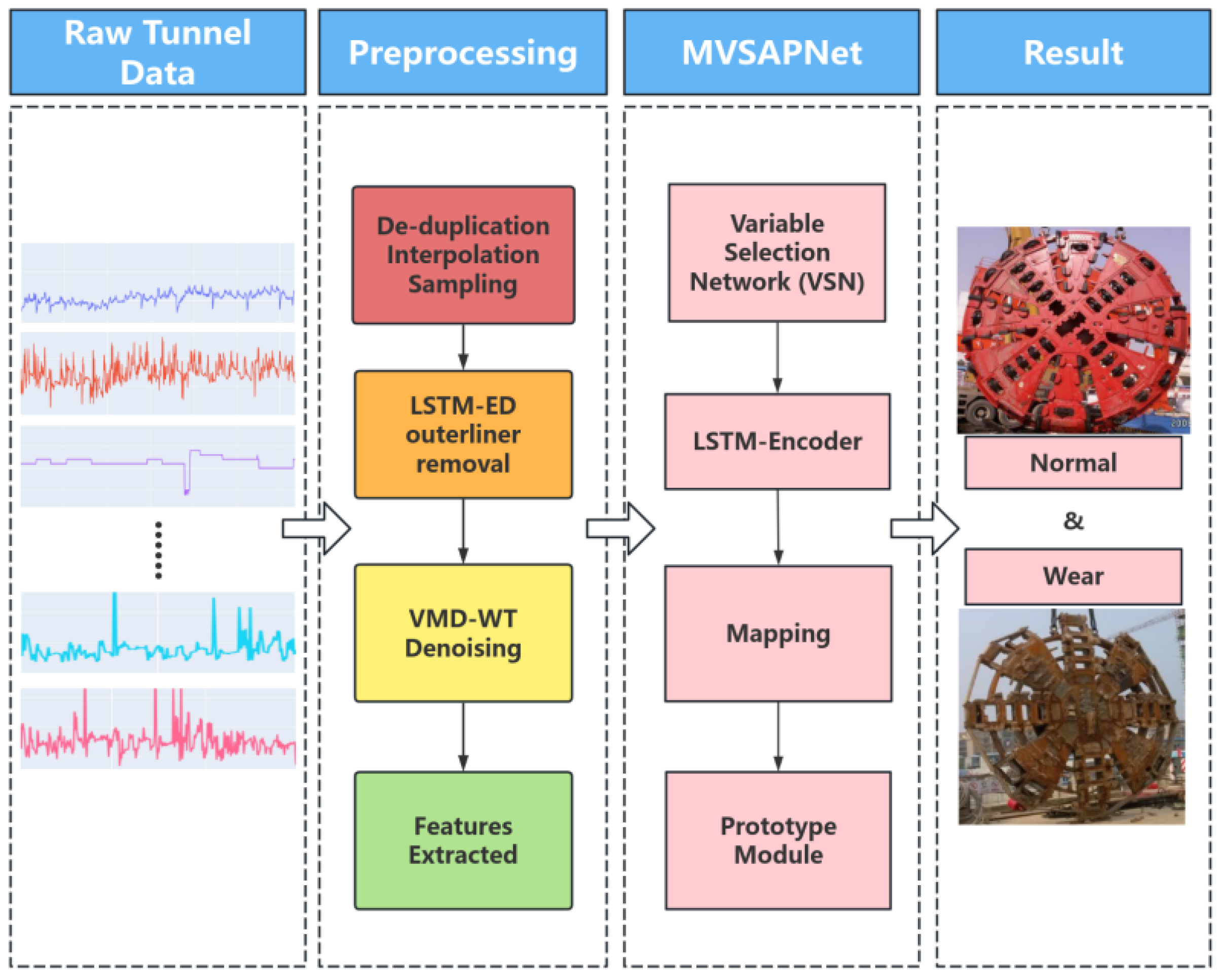
Figure 2.
The architecture of data preprocessing.
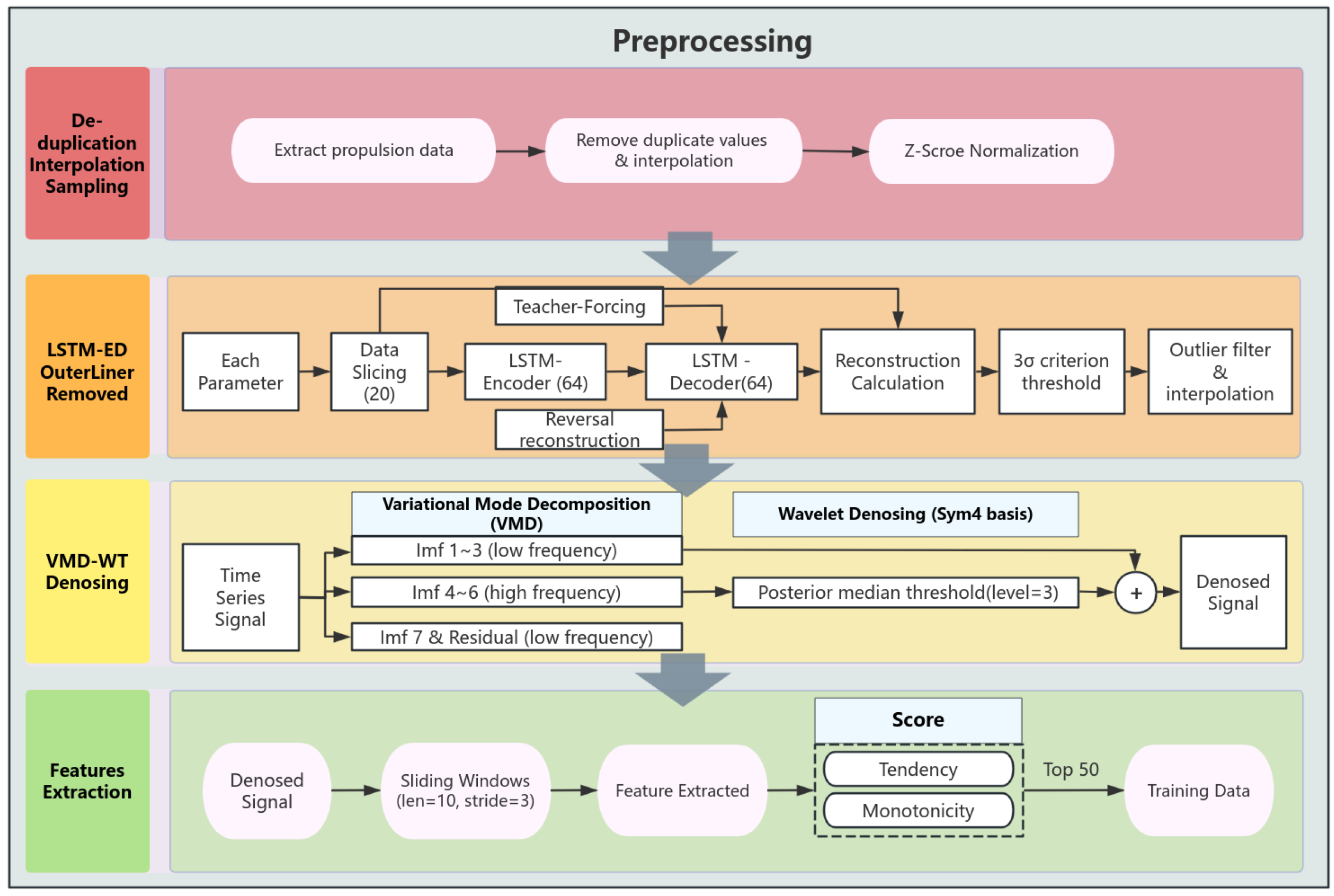
Figure 3.
The architecture of MVSAPNet.
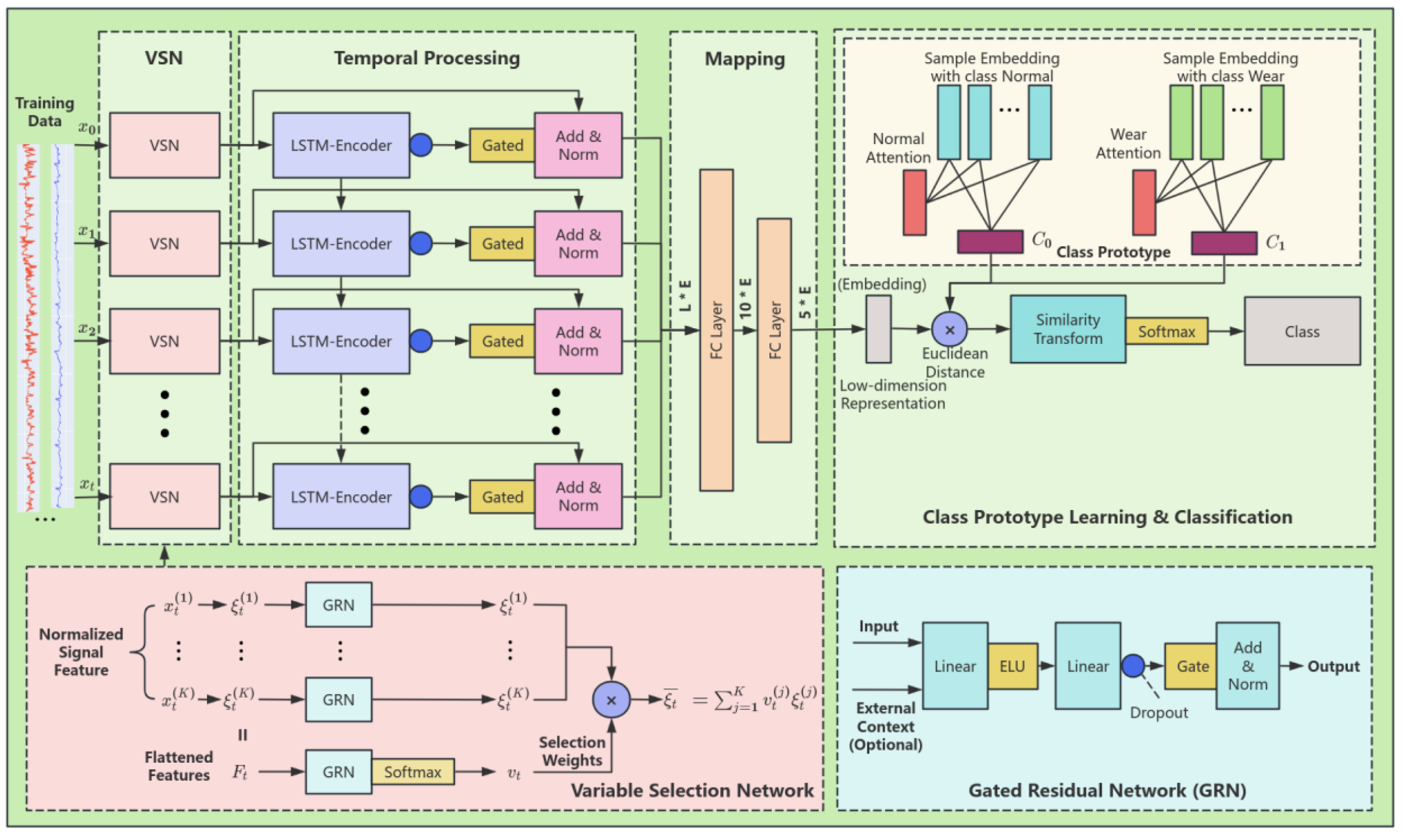
Figure 4.
Outlier removal results for shield disc cutter speed. (a) The blue curve represents the data before outlier removal, the red curve represents the data after outlier removal. (b) the yellow curve represents the reconstruction bias of the LSTM-ED model, and the blue curve represents the use of the selected threshold value.
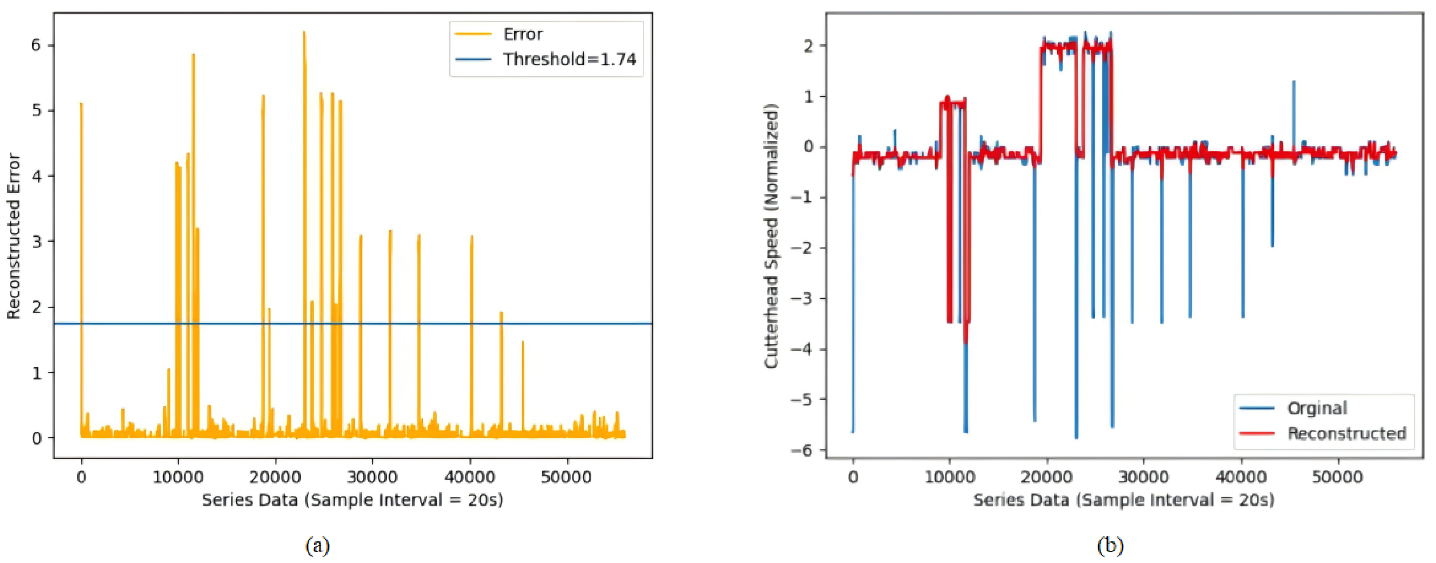
Figure 5.
Denoising results of cutterhead speed using VMD-WT.
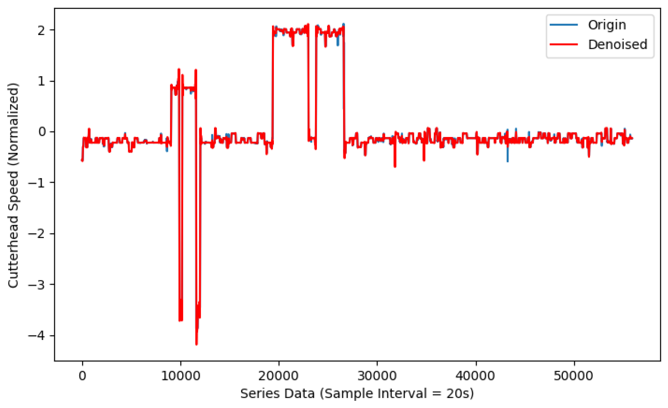
Figure 6.
Effect of different pre-processing steps results with proposed model.
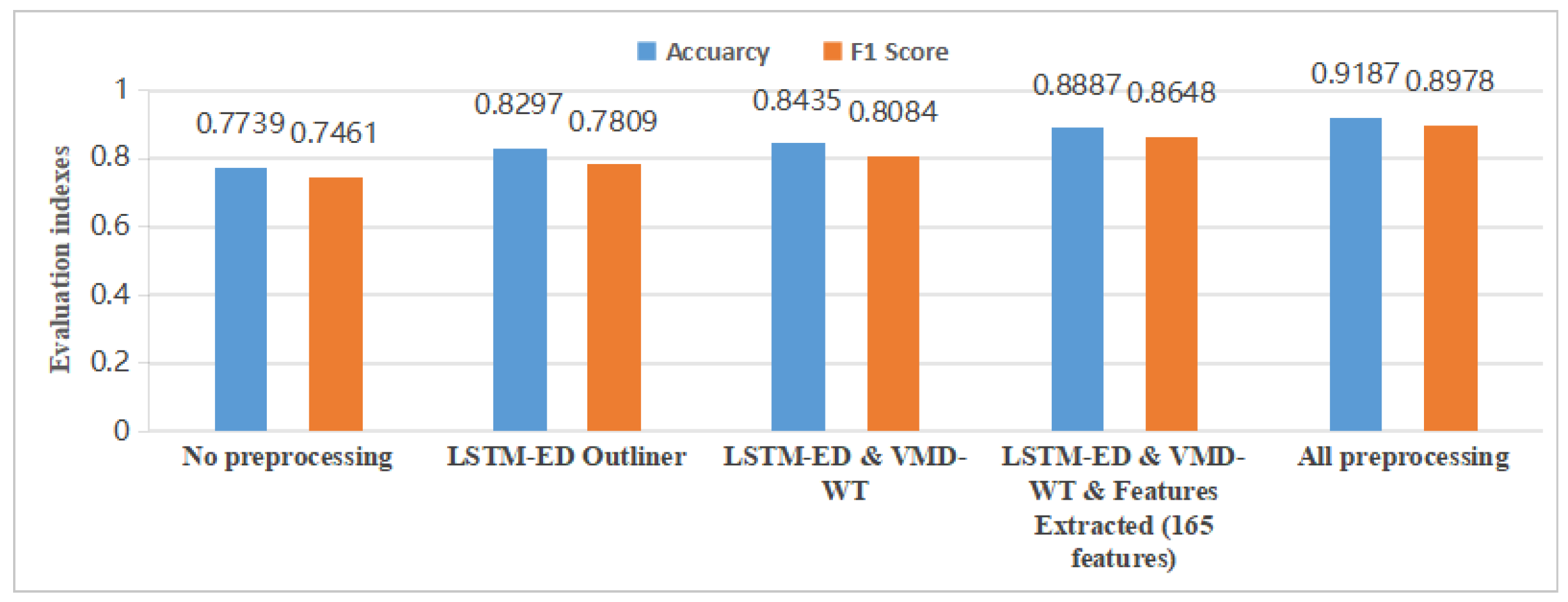
Figure 7.
Impact of removing part of the network structure alone on detection performance.
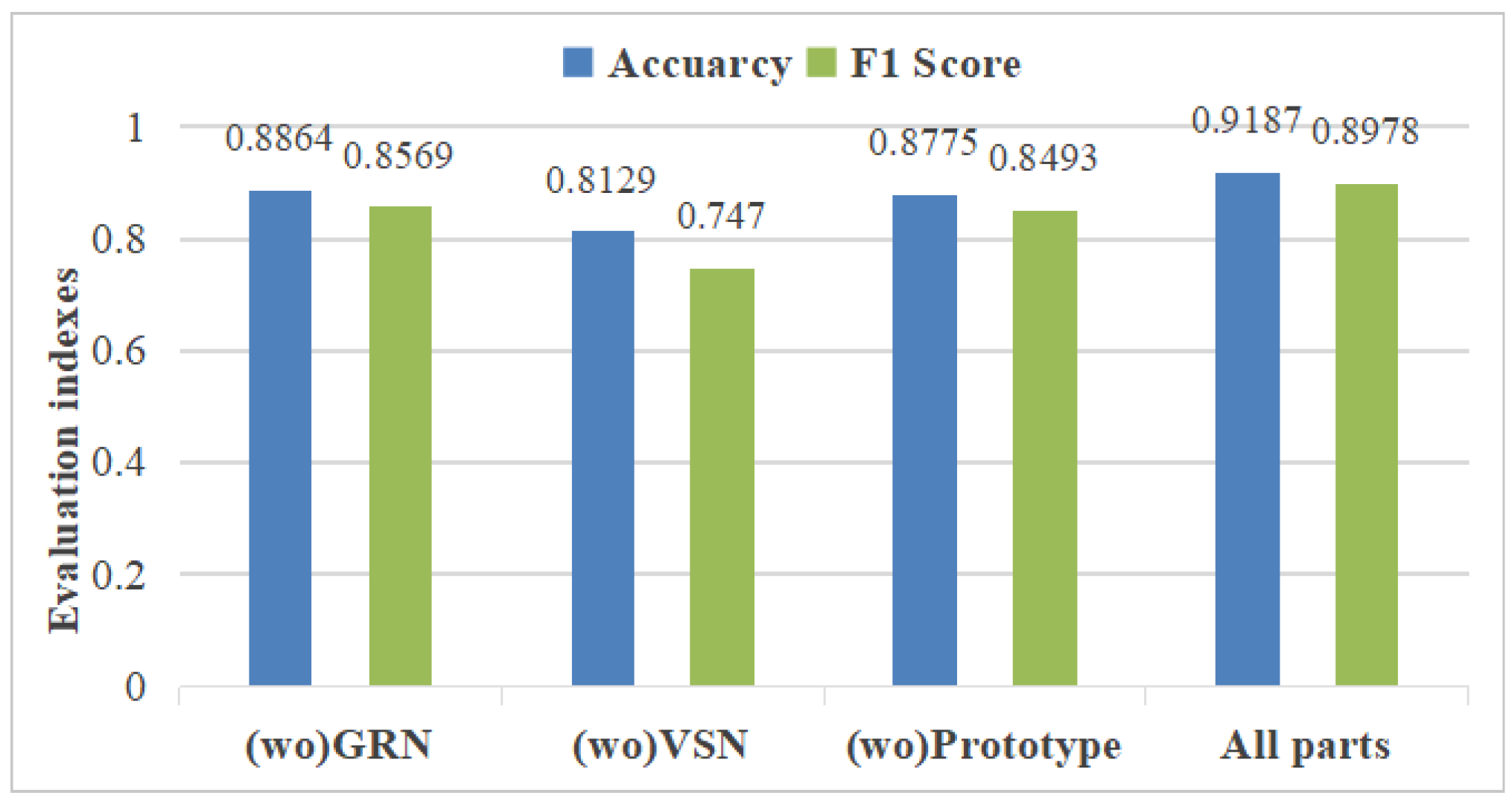
Figure 8.
Visualization of mean weights of in VSN networks.
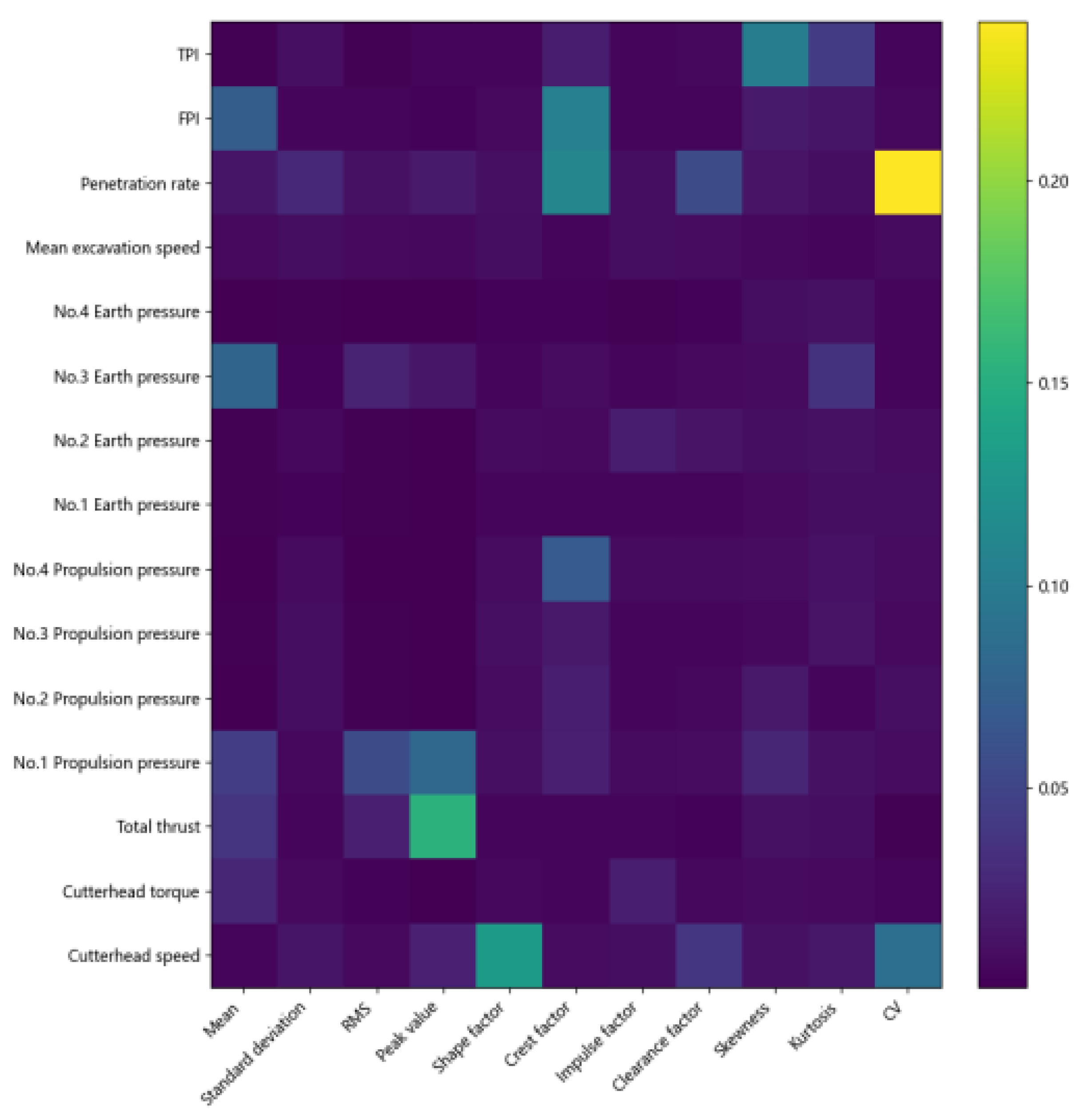
Figure 9.
Visualization results of model sample features and class prototype feature using the t-SNE method, red and black stars for normal and wear state class prototype features, blue dots and orange dots for normal and wear state sample features. (a) Training set. (b) Test set.
Figure 9.
Visualization results of model sample features and class prototype feature using the t-SNE method, red and black stars for normal and wear state class prototype features, blue dots and orange dots for normal and wear state sample features. (a) Training set. (b) Test set.
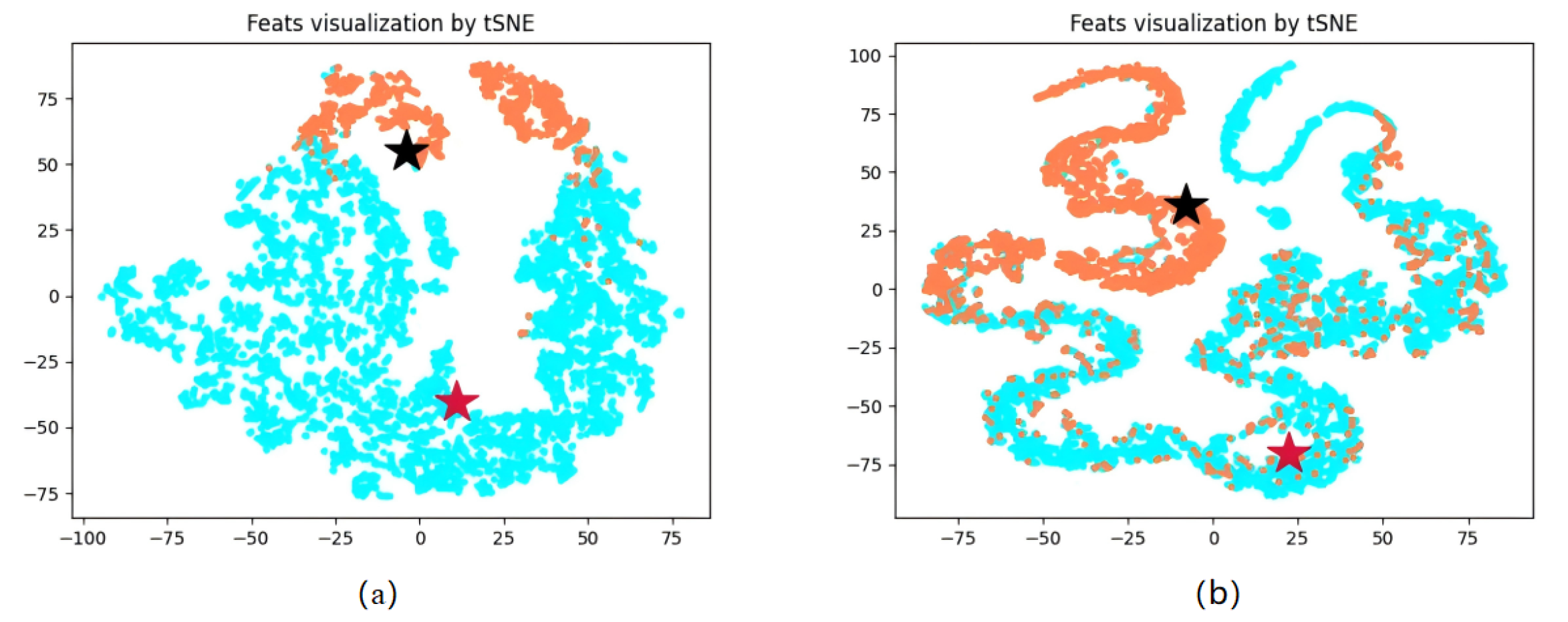
Figure 10.
Visualization results of the distances between the sample vectors and the class prototype matrix on the test set, with the blue line being the distance between the samples and the normal state, the red line being the distance between the samples and the worn state, the green line being the worn distance and the normal distance, and the purple color being the class labels, with 0 = normal state and 1 = worn state.
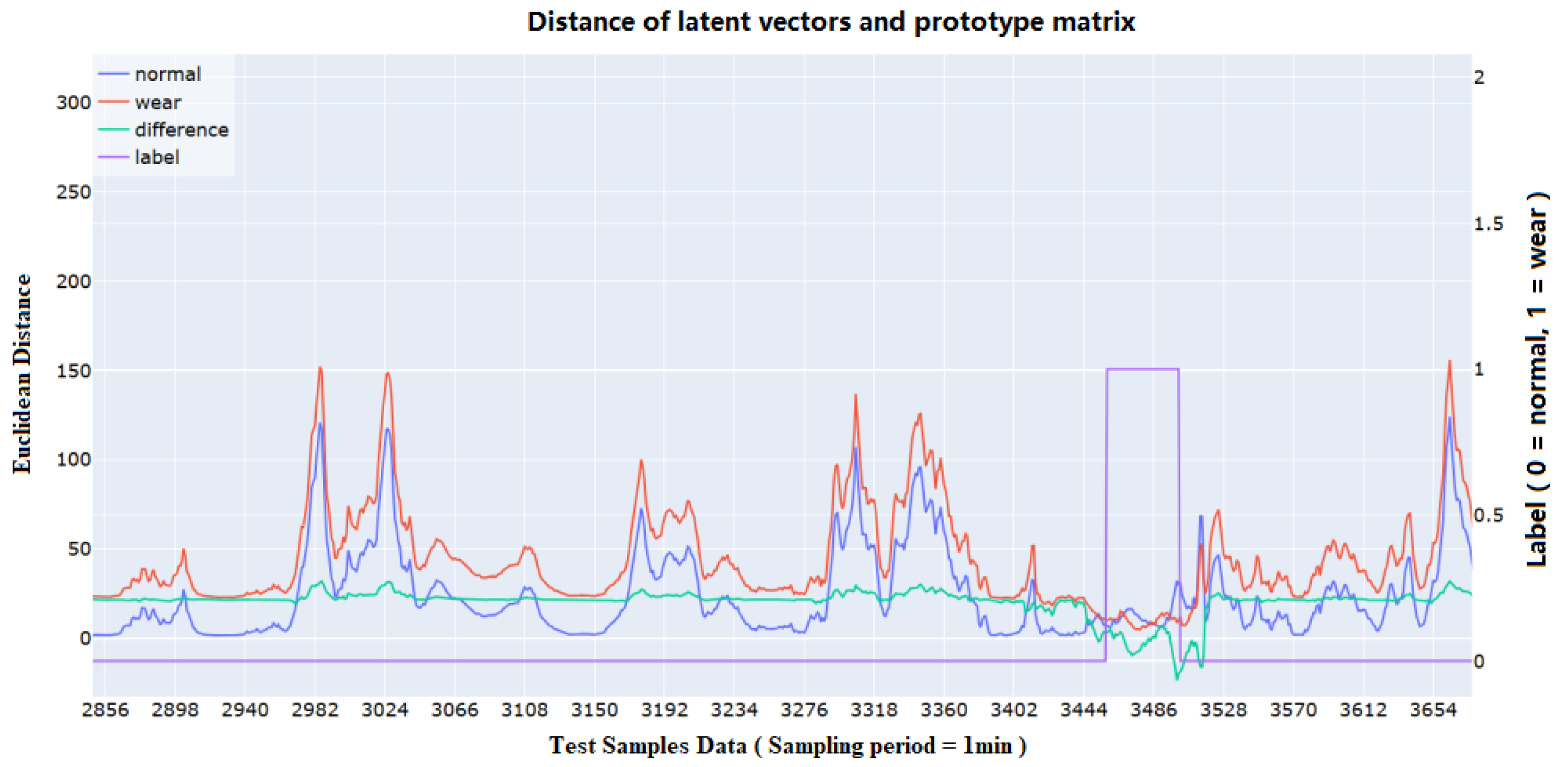

Table 1.
Features selected for feature engineering.
| Index | Feature | Equation | Index | Feature | Equation |
|---|---|---|---|---|---|
| 1 | Mean | 7 | Impulse factor | ||
| 2 | Standard deviation |
8 | Clearance factor | ||
| 3 | Root mean square |
9 | Skewness | ||
| 4 | Peak value | 10 | Kurtosis | ||
| 5 | Shape factor | 11 | CV | ||
| 6 | Crest factor |
Table 2.
Details of 15 parameters selected.
| Number | Parameter |
|---|---|
| 1 | Cutterhead speed (r/min) |
| 2 | Cutterhead torque (kNm) |
| 3 | Total thrust (kN) |
| 4-7 | Propulsion pressure of cylinders groups No. 1-No. 4 (MPa) |
| 8-11 | Earth pressure of excavation soil bin No. 1-No. 4 (bar) |
| 12 | Mean excavation speed (mm/min) |
| 13 | Penetration (mm/r) |
| 14 | FPI |
| 15 | TPI |
Table 3.
Partial results of trend and monotonicity scores for features.
| Features | Monotonicity | Trend | Score |
|---|---|---|---|
| Standard deviation of mean excavation speed | 0.08 | 1 | 1.08 |
| Kurtosis of cutterhead torque | 0.1962 | 1.49e-07 | 0.1962 |
| Skewness of cutterhead torque | 0.1962 | 0.0007 | 0.1781 |
| Standard deviation of Earth pressure No. 1. | 0.0171 | 0.1610 | 0.1781 |
| ... | ... | ... | ... |
| Mean of Penetration | 0.0952 | 0.0358 | 0.1310 |
Table 4.
Performance comparison of different classification networks on test set of disc cutter wear.
Table 4.
Performance comparison of different classification networks on test set of disc cutter wear.
| Model | Accuarcy | F1-Score |
|---|---|---|
| LSTM-FCN | 0.8151 | 0.7917 |
| ALSTM-FCN | 0.8427 | 0.8230 |
| BiLSTM | 0.8422 | 0.8172 |
| ResNet | 0.8385 | 0.8104 |
| InceptionTime | 0.8642 | 0.8412 |
| TapNet | 0.8594 | 0.8350 |
| GTN | 0.8848 | 0.8556 |
| TARNet | 0.9023 | 0.8785 |
| MVSAPNet | 0.9187 | 0.8978 |
Disclaimer/Publisher’s Note: The statements, opinions and data contained in all publications are solely those of the individual author(s) and contributor(s) and not of MDPI and/or the editor(s). MDPI and/or the editor(s) disclaim responsibility for any injury to people or property resulting from any ideas, methods, instructions or products referred to in the content. |
© 2024 by the authors. Licensee MDPI, Basel, Switzerland. This article is an open access article distributed under the terms and conditions of the Creative Commons Attribution (CC BY) license (http://creativecommons.org/licenses/by/4.0/).
Copyright: This open access article is published under a Creative Commons CC BY 4.0 license, which permit the free download, distribution, and reuse, provided that the author and preprint are cited in any reuse.


