State-Space Curvatures and Self-Organizing Criticalities

1. Introduction

The reader is expected to be familiar with the fact that the second law of thermodynamics is often popularized as stating that (a certain class of) systems tend to move from order to disorder (showing an increase in entropy), and that the most notable alleged exception to this is the spontaneous emergence of life-forms (so-called Self-organizing Criticalities (SoC)) [1,2]: somehow life seems to defy this law, at least for a while. This has puzzled scientists in a wide array of sciences for decades, with Schrödingers ’What is Life’ being perhaps the most notable.

Neuroscientist Karl Friston provided a descriptive framework with his Free Energy Principle, stating that living entities, cells, brains, etc (defined by Markov blankets) tend towards a state of minimal free energy, by mirroring its environment [3].

This framework has proven to be extremely successful in describing many biological processes and has been applied to a wide range of disciplines, including machine learning. However, this framework is only descriptive: it does not explain why it minimizes its free energy. As such, a general explanatory or even predictive theory is still being sought after.

Difficulties in Thinking About Entropy

One of the reasons that a general explanatory theory has not been found yet, is that it is very hard to properly think about what is going on. Intuitive notions like ’order’ and ’disorder’ or ’chaos’ are extremely contextual and subjective, and as such this order/disorder-dichotomy is fundamentally flawed and strictly useless for formally describing dynamic behavior in systems. Our biases in looking at systems is so deep that it is very hard to recognize flaws in ones thinking, and in failing to do so some even state that the second law of thermodynamics does not actually hold universally, and should be challenged. Maxwell’s demon is the most famous example of supposedly disproving the Second Law. But this paper argues that it is never the case of a flaw in the Second Law, it is always a flaw in one’s thinking about it.

Most paradoxes come from thinking-errors that concern not properly recognizing ’the closed system’ (Maxwell conveniently forgot that his demon, in monitoring the gas-molecules, is itself actually burning a lot of energy while breathing, sweating, looking, processing, and working the box, let alone its supporting metabolism and even its initial growth and learning to be able to work the box to begin with, which, including all this in the system, easily increases aggregate entropy after all, in full conformance to the Second Law. - As if a demon would do it for free..).

2. Materials and Methods

2.1. Sytems, Micro/Macro-States

We need to think about systems at a higher level of abstraction, in order to be able to generalize what we are talking about. This is done best by the use of the notions of ’microstate’ and ’macrostate’ of a system. The Second Law stating that entropy does not decrease is not so much law, but more a purely a statistical inference: over time it is more likely that a system will occupy a macrostate that has many microstates, than a macrostate will little microstates. This inference actually not only tells you that entropy will increase over time, it also tells you that it will increase as fast as possible (the Maximum Entropy Production Principle) [4,5].

The laws of thermodynamics originally apply to ideal gases. If we want to apply this law to other systems, it is imperative to be strictly precise in what we choose and define as ’the system’ and ’the macrostate and microstate’, and then check if we can define a meaningful entropic gradient over time (for which we can statistically infer that it can never be negative).

2.2. State-Spaces

That can be challenging for many cases, but even more so when it comes to ’living systems’. In the myriad of currently defined types of entropies, ranging from economics to information theory and the physical sciences, the state-space is always a given, a constant, an unchanging environment; the state-space is just the state-space. It is a fixed host.

But in order to explain the ’spontaneous emergence’ that defies the second law, we actually need a generalization of this ’constant state-space’ as a special case of ’a changing state-space’.

Mathematically this translates to a dynamic dimensionality of the state-space, instead of the canonical fixed dimensionality.

In expressing entropy mathematically, that would result in just adding another parameter or function that accounts for the dimensionality of the system at time t, but for a better understanding we will keep using the notion of ’a state-space’ that has its own dynamic, which in turn hosts the state of ’the system’ at hand.

2.3. State-Space Curvature

In a statespace of constant dimensionality it would indeed be impossible for life-forms to emerge and remain stable for some time.

However, if you allow for the state-space (of the life-form) to increase in dimensionality, this provides for an alternative entropic gradient.

And if this dimensionality increases fast enough, this gradient can outperform the ’canonical’ entropic gradient (on which the organism would fall apart). After all, entropy will not only increase, but it will increase as fast as possible.

Such an increasing state-space dimensionality actually occurs by the continuous increase of complexity of a growing organism (new cells, the whole developmental biology process actually, etc), or, for example, the increasing (economic) complexity of a growing economy.

Mathematically, since we are dealing with nonlinear complex-dynamic systems, the increase of complexity can yield chaotic attractors of entropy production. This allows us to introduce the notion of state-space curvature: this increase of complexity can, in ideal cases, provide a curvature-dynamic that ’catches’ the system, just like Einsteins dynamic ’spacetime curvature’ can catch a body of matter.

The analogy sits in that for us observers the moon seems to move in a circle, but it is actually spacetime curvature; and just like that for us observers a living system seems to decrease in entropy, but it is actually statespace curvature.

So a living organism (any SoC actually) does not actually self-organize or self-sustain, but it is being organized/sustained by its statespace-curvature. In other words, the ’hosting system’ provides an increasing entropic gradient.

2.4. The Organism Is Not the System

Although we now have a more generalized view on SoCs which provides a full explanation of its emergence (we generalized the canonical fixed-dimensional statespace as a special case of dynamic statespaces), we still have an issue.

After all: in order for complexity to keep increasing (to maintain the entropic gradient), the organism would need to keep growing. And it is obvious that although most living systems do grow for some time, at some point they actually stop growing, and the entropy of the organism does not increase anymore. So why does the organism not collapse, as soon as it stops growing?

In order to understand this, we have to distinguish between ’the system’ (caught in the state-space curvature) and ’the organism’. Mathematically we can define the system as a constant concept, but the living organism is not a constant entity at all: it breathes, sweats, eats, drinks, etc. Every other second the actual material composition will differ: molecules are constantly being added and substracted from the organism. As such, the organism is not the system. For us humans the difference is imperceivable, but it is critical in order to fully understand what is going on.

The dynamics of the biological composition has a strong analogy with a wave at sea: the top of the wave is analogous to ’the organism’, and this top constantly changes in material composition. If you define ’the system’ to be the organism (the top of a wave) at time $T=0$, then at $T=1$ ’the system’ will only have some of its particles still at the top of the wave, and the rest is flushing away in the sea, in full conformance to the Second Law. ’The organism’ is NOT ’the system’.

We can now understand that the life-span of an organism can be understood as a wave on some state-space curvature, and this analogy even continues until the death of the organisms: mathematically it is the same dynamic as a breaking wave.

2.5. Fractality of Systems

It will be evident that, if we think of a state-space curvature, the state-space itself probably classifies as a complex-dynamic system as well. Choosing what we define as ’a system’ (an organism, a cell, an ecosystem, a tornado, a weather-system, an economic market, etc) is always arbitrary. After all, the dynamics of the system and the dynamics of state-space influence each other, so you can also think of them as a single dynamic system.

You can define ’a tornado’ as a system and then identify the hosting weather-system as a dynamic state-space. In this case it is clear that determination of which molecules would be part of the tornado-system is futile: it would change every microsecond. This is the reason that the mathematical field of nonlinear, complex dynamic systems does not deal with particles or cells or entities, but only with their dynamics. And these dynamics can show patterns like chaotic attractors, and classifiable bifurcations. This actually tells us that what we think of as the conception and death of a discrete organism, are actually bifurcations within the larger, hosting complex-dynamic system (an ecosystem). From this systems-perspective there is no discrete organism., but only an complex-dynamic system with myriads of chaotic attractors of bifurcating into and out of existence, like eddies in a river.

That helps us to overcome our bias (from the human perspective and scale) on what is generally meaningful to define in order to get a better understanding.

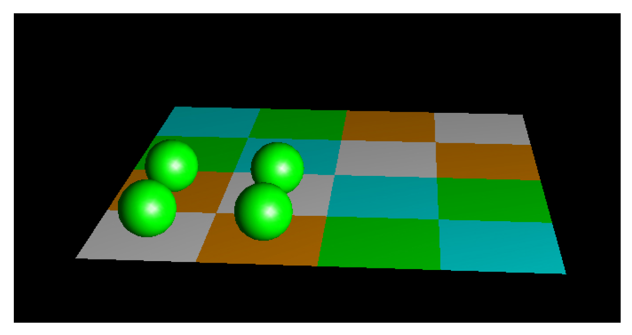
2.6. Simple Calculation

To demonstrate for a simple system that the entropy gradient towards a higher dimension exceeds the gradient in the same dimension, consider a system of 4 marbles within a 2D state-space of 4x4 cells. The entropic gradient is the difference between $S_{min}$ and $S_{max}$.

For this system the entropy S can be calculated by the simple formula S = ln W, where W is the number of microstates that correspond to a macrostate (quadrant-based even distribution).

The lowest entropy that this system can have equals the entropy of least freedom, e.g., all in a corner. This yields

$$W_{min,2D}=4\times 3\times 2\times 1=24$$

permutations.

Figure 1. Minimum entropy.

Figure 1. Minimum entropy.

The highest entropy, all within their own quadrant with maximum freedom, yields

$$W_{max,2D}=16\times 12\times 8\times 4=1660$$

possible permutation .

Figure 2. Maximum entropy.

Figure 2. Maximum entropy.

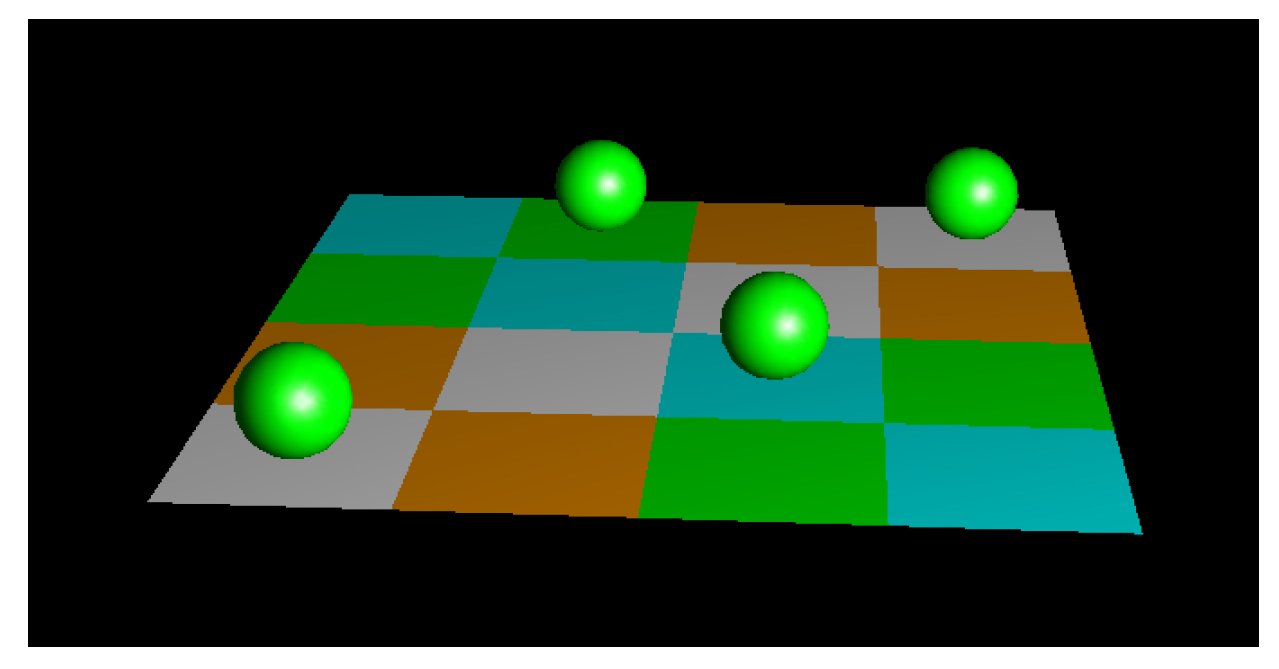
The entropy-gradient

$$d{S}_{2D}=S_{max}-S_{min}=ln\left(1660\right)-ln\left(24\right)\approx 4.2$$

For the 3D-case, we have a grid of 4x4x4. Again, the lowest entropy possible is given by all the 4 marbles in some corner, yielding

$$W_{min,3D}=6\times 5\times 4\times 3=360$$

solutions. If we seperate the cubic structure into 4 equals parts, the marbles will have maximum freedom. First marble can choose from 64 options (claiming 1 cubic quadrant), second has 48 left, third has 32 left, last quadrant leaves 16 options, so a total of

$$W_{max,3D}=1,572,864$$

permutations. The gradient

$$d{S}_{3D}=S_{max}-S_{min}=ln(1.572.864)-ln\left(360\right)\approx 8.3$$

In other words: it is much more likely that the system will traverse into the 3D-grid, than that it will remain within the original 2D-grid. The degree of freedom increases with an increase in dimensionality of the statespace.

3. Results, Applicability

This paper has provided a generalization of the thermodynamics for complex-dynamic systems. The applicability of this generalization is not limited to ’living systems’. It also applies to other domains, such as weather-systems: for example: a tornado does not self-organize, but the hosting weather-system provides the entropic gradient that provides for a chaotic attractor for nonlinear dissipation of temperature/pressure/humidity differences. The tornado emerges and dies like a wave in the sea. Of course the dimensionality of the state-space for living organisms is orders of magnitudes higher than the dimensionality of the tornado, but the mathematical principle is exactly the same.

Another application concerns ’the economic system’, ranging from transactional micro-market-structures (the quant-domain) to traditional economic growth and macro-economics. Yes the economic system has thermodynamic aspects. Not concerning entropic dissipation of money (this does not hold), but transactional entropy concerning settlement of suppy and demand: a market-system ’wants’ to settle (dissipate) supply and demand as much and as fast as possible. Chaotic non-linearity optimizes through infrastructural clustering of settlement (exchanges) and (with higher dimensionality from increasing complexity (IT-revolution)) even bifurcating towards temporal clustering of settlement (High Frequency Traders).

Also, recently, a lot is going on around solving the black hole paradox in relation to entropy, for which state-space curvature through increase of complexity provides a full explanation.

4. Discussion

Some complex-dynamic systems are actually fundamentally driven by maximizing entropy, but at a high level of abstraction. Recognizing this can provide a much better understanding of their behavior.

The generalization of the state-space of a system as a special case of dynamic state-spaces allows us to introduce the notion of state-space curvature, which can provide for a specific entropic gradient in dimensionality for the state of the system, which outperforms the ’canonical’ entropy gradient, which would degrade the system towards (disorder), and as can yield and sustain an ’orderly’ state of a system.

This synthesis of the statistical Principle of Maximum Entropy Production and complex-dynamic systems provides for a fully explanatory framework for the ’spontaneous’ emergence and sustainability of emergent, orderly patterns in non-linear, chaotic systems, that is widely applicable.

References

- Bouchoud, J.P. (2024). The Self-Organized Criticality Paradigm in Economics and Finance. [CrossRef]
- Dewar, R. (2003). Information theory explanation of the fluctuation theorem, maximum entropy production and self-organized criticality in non-equilibrium stationary states. Journal of Physics A: Mathematical and General, 36(3):631–641. [CrossRef]
- Ramstead, M. J. D., Badcock, P. B., and Friston, K. J. (2017). Answering Schrödinger’s question: A free-energy formulation. Physics of Life Reviews, 24:1–16. [CrossRef]
- Martyushev, L. M. (2010). The maximum entropy production principle: Two basic questions. Philosophical Transactions of the Royal Society B: Biological Sciences, 365(1545):1333–1334. [CrossRef]
- Veening, M. (2021). A Statistical Inference of the Principle of Maximum Entropy Production. https://www.preprints.org/manuscript/202103.0110/v1.
Disclaimer/Publisher’s Note: The statements, opinions and data contained in all publications are solely those of the individual author(s) and contributor(s) and not of MDPI and/or the editor(s). MDPI and/or the editor(s) disclaim responsibility for any injury to people or property resulting from any ideas, methods, instructions or products referred to in the content. |
© 2024 by the authors. Licensee MDPI, Basel, Switzerland. This article is an open access article distributed under the terms and conditions of the Creative Commons Attribution (CC BY) license (http://creativecommons.org/licenses/by/4.0/).
Copyright: This open access article is published under a Creative Commons CC BY 4.0 license, which permit the free download, distribution, and reuse, provided that the author and preprint are cited in any reuse.