
Submitted:
20 December 2024
Posted:
23 December 2024
You are already at the latest version
Abstract
The research area of NILM exhibits a high heterogeneity, regarding approaches and characteristics. Especially, in terms of the applied algorithms, measurement data, quantities and features used, as well as congruent appliance event and state definitions. Therefore, performance evaluation and the establishment of comparability is not straightforward. The aim of the presented work was to address these challenges, through the development of an application-oriented, general methodology for parametrization, optimization and performance evaluation of NILM algorithms. The methodology is based on the general NILM framework and applicable to a wide range of NILM approaches and measurement data. Temporary, individual appliance measurements were utilized to build an extended appliance database and for providing a reliable ground truth for common performance evaluation metrics. Therefore, also a congruent event and state definition was formulated. For the application of the methodology, the focus was set on event-based NILM algorithms and measurement data of a commercial building and for one significant appliance, regarding the building´s overall energy demand. The methodology proved to be suitable for the aimed purpose. Two different event detection algorithms could be optimized, regarding their input parameters to be able to identify the appliance operation behavior optimally.
Keywords:
Non-intrusive load monitoring (NILM)
; disaggregation
; performance evaluation
; commercial and industrial buildings
; event detection
1. Introduction
The consequences of ongoing climate change can already be seen all over the world. Next to the extension of renewable energy generation, increasing efficiency in energy use can contribute substantially to lowering CO2 emissions. In the building sector, the research area of non-intrusive load monitoring (NILM) deals with the identification of individual electrical appliance behavior within the load profile of buildings or building sections, without the need for expensive individual measurements [1]. The energy efficiency potentials of buildings can thus be identified and quantified in a highly economical and cost-effective way. Other areas of application are appliance fault detection, demand side management, energy demand forecasting and billing [2,3].
The general NILM framework can be divided into the steps of data acquisition, appliance feature extraction and inference and learning [4]. The step of inference and learning is also referred to as load identification [5]. Figure 1 visualizes the typical elements of the general NILM process. To be able to assign extracted appliance features to specific building appliances in the stage of load identification, features of these appliances have to be known in some form in advance. This information is often provided by appliance databases [5,6]. The extent of information and data within appliance databases is depending on the characteristics of measurement data, as well as the applied NILM algorithms and their necessary features for load identification. In this work, a general methodology is developed for parametrization, optimization and performance evaluation of NILM algorithms. Thereby, optimal NILM algorithms, parameters, as well as appliance models and optimal identification features can be derived and provided to the general NILM framework using an extended appliance database approach, compared to literature.
NILM approaches can be categorized into event-based and eventless NILM methods. Eventless NILM can also be referred to as non-event-based or state-based NILM [7,8]. In event-based NILM, event or edge detection is performed in the step of feature extraction, to identify individual appliance’s state changes or transients. Event detection can be seen as an individual process step in NILM as well, e.g., as in [9]. Feature extraction and load identification is then performed for the detected events, only. In eventless NILM approaches, on the other hand, building appliance models are used, e.g., through state machines or functions, to disaggregate the building’s load profile [7]. In this case, every sample of data acquisition is taken into account directly for feature extraction and load identification [8]. Appliances and data acquisition are often considered regarding their active power behavior, but also other measurement quantities are used in NILM, e.g., reactive power, current or voltage. In eventless NILM these quantities are directly used as features, while in event-based NILM features consist of characteristics of detected events, e.g., absolute changes in active power, caused by events. Therefore, in this work, we differentiate between measurement quantities and features.
Depending on NILM approaches and algorithms, sampling rates and data resolutions of the aggregated data acquisition (aDAQ), measurement quantities and features are varying. Sampling rates may start at 1 Hz or lower, and can range up to 20 kHz and more. Usable features are depending on these sampling rates. Examples for low sampling rate features are RMS values of active and reactive power, higher sampling rates are necessary, e.g., for the analysis of the harmonic spectrum. Wavelets and electromagnetic interferences can be used as features with sampling rates starting at 20 kHz [10]. Especially for power quality meters, sampling rates and data resolutions are not identical. These meters usually operate with sampling rates around 20 kHz, but measurement quantities can be read out, e.g., with minimum resolutions of 5 samples per second (S/s).
Appliance models are used in certain NILM approaches, in the step of feature extraction or load identification. Therefore, typical appliance characteristics were categorized in literature, to be able to create suitable appliance models. Usually, load signatures regarding active power or current are taken into account for categorization. Frequently used categories, e.g., in [10]. and [11], are on/off or single-state appliances (mostly resistive loads, e.g., non-dimmable lighting), permanent consumers (e.g., network switches) and multi-state devices (e.g., washing machines), representable by finite state machines (FSM). Furthermore, continuously variable devices, not having constant steady states (e.g., dimmable lighting) and non-linear devices with strong variations within their states (electronic devices, e.g., PCs) were identified [12]. distinguishes resistive, inductive, capacitive and non-linear appliances, as well as composite loads, being a combination of the prior. Besides on/off appliances, in [13]. the following models are named: On/off decay or growth, additionally having a growth or decay component, stable min-max, with a stable baseline and short power deviations, and random range devices, exhibiting a power range with random variations. A superposition of these models are compound appliances [14]. differentiates category (e.g., corridor lighting) and device models (individual appliances). Factorization-based equations are used for current modeling. Adaptive energy models are used in [15]. for manufacturing industries, derived from machine control signals and energy measurements. In our approach, FSM-based appliance models are used, where transients and steady states can exhibit various features, regarding the measured quantities. E.g., if a certain appliance state is continuously variable, we interpret this as a specific state with a certain power range. More details on appliance models can be found in section 2.
Eventless NILM approaches show a lower disaggregation granularity compared to event-based approaches, being able to detect most of the significant appliances, using sampling rates up to 1 kHz. Event-based approaches exhibit higher disaggregation accuracies, using higher sampling rates, according to [16]. [17] states however, that eventless approaches are more accurate, and can handle appliances with long unchanged states. According to [8], event-based approaches are computationally more efficient and show better performance [18] states generally, that higher sampling rates are leading to higher detection accuracies by minimizing simultaneous events [19] highlights the advantageous model complexity of event-based approaches. Further benefits of event-based approaches are named: Fewer computation resources, a more rapid response and an easier application in practice. Therefore, these approaches are seen as more promising. The beneficial robustness to noise is added by [17]. [20] states that eventless approaches are more practical and valuable for industrial users and emphasizes the capability of real-time monitoring. As can be seen, literature does not give a clear indication to prefer one approach over the other. The methodology, presented in this work, was therefore not limited to event-based or eventless approaches. Yet, in the application of the methodology, later in section 4, we use event-based NILM algorithms. Therefore, event-based NILM is described in detail in Section 1.1.
The complexity of NILM algorithms shows great variations and achieving comparability and evaluating performance of NILM algorithms is not straightforward. Many performance evaluation metrics have been applied in the field of NILM. In [21], the authors give a comprehensive overview and classify literature approaches into event detection metrics, used for performance evaluation of event detection algorithms, and energy estimation metrics, usually applied to eventless approaches or the overall NILM process. The confusion matrix is a frequently applied metric in the event detection metric category, where detected events are classified as correctly detected (true positive – TP) or misdetected (false positive – FP). The remaining load profile segments can be divided into correctly identified steady states, not containing events (true negatives – TN), and missed events (false negatives – FN). Well known representatives of the energy estimation category are statistical measures, like the relative error or the root mean square error, or energy related measures, e.g., the energy error. In this case, the actual load profile is evaluated against the part of the load profile, assigned to individual appliances by certain NILM algorithms. For event detection metrics it is necessary to have a clear and congruent event and state definition. All performance evaluation metrics strongly rely on measurement data or datasets providing a suitable ground truth, giving information about the actual individual appliance operation within aDAQ data.
More than 30 datasets have been published so far in the area of NILM. These datasets contain measurements for the aggregated consumptions mostly of households, more recently also from commercial or industrial buildings, or parts respectively. Some datasets present measurements of individual appliances additionally or exclusively. Due to different measurement approaches and areas of application, they show great contrasts regarding contained data. Some examples are the measurement duration, sampling rates and data resolutions, included features and additional information about individual appliance operation and data formatting [1,21]. Examples for frequently used datasets are BLOND [22], BLUED [23], COOL [24], SustDataED [25]. or UK-DALE [26]. Comprehensive overviews of the various datasets can be found in [11] and [21].
In recent NILM research, more focus was set on machine learning and non-household applications for commercial and industrial buildings. An overview of machine learning approaches can be found in [2], [9] and [11]. Exemplary applications are provided by [19] and [27]. Industrial applications of NILM can be found in [20] and [28]. In this work, we apply measurement data of a commercial building, as we see the necessity to further investigate the application of NILM in non-household buildings, due to the high potential for energy efficiency improvement. In section 1.1, event-based NILM is described in detail.
1.1. Event-Based NILM
As described above, the basis of NILM is an aggregated measurement of a certain quantity of individual appliances, e.g., of a building or a building section. From this measurement, certain measured quantities are evaluated, e.g., active or reactive power, current and more. In event-based NILM, the samples i from the measured parameter x[i] are examined by event detection algorithms, to determine the presence of events, with i = (1, 2, …, k). These events can then assigned to state changes of individual appliances. In literature, a lot of event detection algorithms have been applied so far. They can be categorized in expert heuristics, probabilistic models and matched filter models [9]. Frequently used event detection algorithms are the method of cumulative sums (CUSUM) [29], the generalized or log likelihood ratio (GLR or LLR) or the cepstrum method [30], amongst others. In this work, we focus on the χ² test of goodness of fit (χ²-GOF), which can be assigned to the category of the probabilistic models, as well as one method, newly applied to the area of NILM. To demonstrate the scope of our work, we used one well-known and widely applied algorithm, as well as one new algorithm.
χ²-GOF is a statistical method to determine, whether a set of data could reasonably have originated from a given probability distribution [31]. Applied to NILM, this test is used to estimate if an event occurs between two consecutive windows of a time series, the pre-event window p and the detection window q. Each window contains n samples of the measured parameter x. The χ²-GOF test is carried out for every sample i, according to the following equations: [30,32]
If the two windows pi and qi do not share a common probability distribution, an event is concluded at the location i. This is the case, when the test statistic lGOF,i exceeds a certain threshold in the distribution χ²α,n-1. The threshold is represented by the critical value χ2c, depending on the desired confidence interval pGOF = 100 (1-α) % and n-1 degrees of freedom, whereby n represents the window size. In literature, tables can be found that specify χ2c values, depending on the degrees of freedom, often from 1 to 100, and for pGOF values of 90, 95 or 99 %.
Researchers provided variants and improved versions of χ²-GOF, e.g., [30] introduced a voting mechanism for χ²-GOF to improve its robustness against changes in base load. A voting window is applied to the resulting test statistic time series, inspired by the improvements for GLR in [33]. A surrogate-based model is also suggested in [30] to be able to optimize model parameters. In this work, we apply the basic version of χ²-GOF, as described above. To demonstrate the scope of the methodology of this work, we additionally applied one new event detection algorithm, which can be assigned to the category of expert heuristics. This rather simplistic algorithm is derived from the webster’s method, developed for the detecting discontinuities (DSC) in data series. The method was applied to ecological data series before, for example. Based on the two consecutive windows p and q, defined in Equations (1) and (2), DSCs are calculated according to Equation (4): [34]
For each sample i of the measured parameter x[i], mean values are calculated and subtracted for the two windows of the size n. If the absolute value of this difference lDSC,i exceeds a certain threshold, an event is assigned for the data point i.
When talking about event-based NILM and event detection algorithms, it is necessary to discuss event definitions, used in literature. Generally, steady states and transient states are differentiated [4]. Transient states can also be referred to as state changes or transients. In this work, we use transients, when speaking of appliance steady states changing from one to another. The terms events and transients are often used synonymously in NILM. Other appliance or load profile characteristics, e.g., peaks, short pulses and long variable load intervals are referred to as events, as well, e.g., in [35]. Further characteristics, named in literature, are fluctuations [38], edges [36,37] and variations in power or current [16], amongst others. As described above, in the section of appliance characterization, some categories of appliances can exhibit the before named characteristics in steady states as well (e.g., stable min-max devices). When using the terms transient and event synonymously, steady states cannot contain these types of events by definition. Nevertheless, detecting these characteristics in the aggregated load profile can be used in NILM for the identification of appliances’ transients or steady states. As can be seen, proper and congruent event and state definitions are important, especially when it comes to performance evaluation and comparison of NILM algorithms, whether being event-based or eventless.
Event definitions in literature can be classified into three categories:
- ›
- Explicit event definitions
- ›
- Steady state definitions or implicit event definitions
- ›
- Rule- or algorithm-based event definitions
Explicit event definitions are very concrete, mostly referring to the operational characteristics of individual appliances [38] defines an event as an appliance state transition to on, off or other states [39] specifies state transitions as actions that normally include turn-on, turn-off, speed adjustments, and function or mode changes [16] defines an event in a more general way, namely as any state change of an appliance over time. A major disadvantage of these event definitions is the lack of knowledge about the operational behavior of individual appliances. The actual operational states of appliances are often unknown, even if individual measurements are provided, e.g., through datasets. Especially when it comes to complex appliances, it can be hard to obtain information about the actual behavior. This problem is also illustrated in Section 2.
Implicit event definitions refer to steady states rather than events. Non-steady state regions of the load profile can then be interpreted as events [40] defines an event as a change of a signal from an old to a new steady state. This definition is mainly appropriate for on/off and FSM appliances, according to [35]. For this reason, the authors of [35] define an event as an active section where the signal is somehow deviating from the previous steady state. The active section lasts as long as no further steady state has been reached. Implicit event definitions are more general, including load peaks, short pulses and long variable intervals within the load profile. The application of these definitions can be a question of interpretation.
Rule- or algorithm-based event definitions provide clear rules to define the presence of events. In [36], steady states are defined by a minimum duration of 3 s and a minimum power tolerance of 15 W or Var. All other periods are marked as periods of change, containing events. In the BLUED dataset, events were defined, as a change in power, greater than 30 W, lasting at least 5 s [23]. An example for algorithm-based event definitions can be found in the dataset SustDataED, where a version of the event detection algorithm GLR was used for event labeling [41]. The FIRED dataset provides a semi-automatic labelling for events, using a modified version of the event detection algorithm LLR [42]
In [43]. a distinct appliance event or steady state definition is avoided and replaced by an event detection system, using adaptive training to learn from previously wrong detected events. In this case, it is necessary to provide a dataset to the system, where the events have to be labeled manually by the user. The advantage of the approach is, that the problem of event definition can be solved application-specific. It is possible to define and label events of interest beforehand and provide a training dataset to the system.
1.2. NILM Tools and Frameworks
Besides datasets, several tools and frameworks have been published, with the objective to provide comparability and benchmarking for NILM algorithms and approaches. The most popular open source toolkit is NILMTK [44]. Various NILM algorithms, datasets, statistics and evaluation metrics have been implemented, besides data processing tools [45]. NILMTK is being constantly updated, e.g., in [46]. A framework to generate and label NILM datasets has been presented in [42]. As described above, in the semi-automatic approach, modifications can be made with the tool annoticity [47]. Recently, [48] presented a framework for providing explainability in NILM, using explainable AI.
1.3. Challenges, Aim and Objectives
The standardization of performance evaluation, to enable a proper benchmarking is one major challenge in NILM, according to [2]. and [45]. As described in Section 1.1, the research field of NILM exhibits highly heterogeneous characteristics of datasets and measurement data, quantities and features, depending on the different NILM algorithms and approaches used, as well as varying or unclear event or state definitions, applied to a wide range of performance evaluation metrics. Most of the NILM research is based on residential building data. Due to the high potential for energy efficiency in industrial and commercial buildings, this area should be a central aspect of NILM research in future. Furthermore, major challenges for the detection performance of NILM algorithms are simultaneous appliances’ switching events, noisy data and the presence of renewable energy sources. Also according to [2], NILM algorithms need to be trained with appliance sets of the particular building to achieve good performance. High-performing algorithms are tested only on a laboratory scale with high-performing computing devices. Therefore, generalization of NILM approaches and performance evaluation should be in the focus of further research [45]. Furthermore, the need for application-oriented [2] and explainable NILM solutions, especially when AI-based algorithms are highlighted [45].
Based on literature and related work, described in the previous sections, as well as the challenges in NILM, described above, we formulated the aim and the main objectives of the presented work.
Aim:
- ›
- The aim of this work is to develop an application-oriented, general methodology for performance evaluation and optimization of NILM algorithms, applicable to a wide range of NILM approaches.
Objectives:
- ›
- The methodology should enable the application of the common performance evaluation metrics and should base on congruent event and state definitions.
- ›
- The methodology should be based on the general NILM framework, to ensure applicability to a broad range of approaches. Therefore, the concept of an appliance database should be specified and potentially extended, to provide algorithms, parameters, identification features and appliance models to the regular NILM process.
- ›
- The methodology should be applicable to different characteristics of measurement data as well as common NILM datasets, regarding sampling rates and data resolutions, measured quantities, features and appliance signatures.
- ›
- Individual appliance measurements should be used in a temporary learning phase of the methodology, providing a reliable ground truth for performance evaluation.
- ›
- The methodology should be able to consider challenging identification issues in NILM, e.g., the presence of renewable energy sources, disturbances, noise or simultaneous switching events.
- ›
- The concept of the methodology should contribute to the improvement of the explainability of algorithms and approaches, e.g., also the application of AI in NILM.
- ›
- Furthermore, the methodology should be applied to event-based NILM algorithms and measurement data of a commercial building, exemplary.
The NILM methodology, developed in this work, is described in detail in Section 3. After that, the methodology is applied to event-based NILM algorithms, using real-world measurement data of a commercial building in Section 4. As a basis of the methodology, our event and state definition statement is presented in the following Section 2.
2. Event and State Definition
A main objective of this work is to develop a consistent event and state definition, as a basis for the methodology for performance evaluation and optimization of NILM algorithms. A discussion of existing event and state definitions in the field of NILM can be found in Section 1.1. We use an application-specific state definition. Depending on the area of application, useful appliance models should be created by differentiating the appliance behavior into steady states and state changes, referred to as transients. Models can be built using different measured quantities, but must be congruent and complete, in order to display the appliance behavior properly, in the way it should be identified later through NILM algorithms, depending on the desired application. Events are defined independent of states and transients. We use the following definitions:
State definition: States are defined as regions in the time series of one measured parameter, or more, where the appliance behavior is stable, regarding the desired area of application.
Event definition: Events are defined as characteristics of one measured parameter, or more, that can be used in NILM to identify certain appliance states or transients.
In Figure 2a, the aggregated active power consumption is shown for two appliances exemplary, in order to illustrate this event and state definition. In this work, we apply NILM algorithms for the disaggregation of a buildings energy consumption. Therefore, the appliance models are derived from, and should properly display, the active power behavior of appliances. For the figure, two appliances from BLOND dataset [22] were used to generate an aggregated load profile. The methodology of load profile modeling using high-frequency appliance measurements is described in detail in [1]. States and transients, according to the described definition and application, are shown in Figure 2b, for the two appliances each. The computer changes it’s state from off to on at t = 25 s and from on to off at about 58 s, as can be seen in Figure 2a,b. Even though the on-state exhibits short power deviations, we define this as a steady state. In our definition, events include all types of discontinuities in specific features (e.g., active or reactive power, current harmonics, etc.), which are useful to identify steady states or transients of individual appliances. This event definition also includes peaks, pulses, fluctuations, etc. The power fluctuations of the computer’s on-state can therefore also be defined as events. The on- and off-transients of the computer, in this case, correspond with one event each. This is different for the operational behavior of the projector.
The startup-process of the projector begins at 1 s, corresponding with the beginning of the transient from the off- to the on-state. At about 68 s, the appliance reaches a steady on-state, regarding it’s energy consumption. The transient from on to off lasts from 75 s to 81 s. According to the definition, described above, both transients can exhibit events. But, as explained above, the goal of NILM algorithms is to identify states and transients of certain individual appliances. The performance of this identification process is evaluated within our methodology, whether using one event, several events or no events, in the case of eventless NILM, to do so. In the case of the projector in Figure 2a, an event detection algorithm could identify the whole section from 1 s to 12 s as one event, or detect three or more events in this area, concluding a state-change of the projector. In both cases, we would evaluate the performance of the algorithm equally positive.
The interpretation of events depends strongly on the characteristics of the measurement, e.g., the sampling rate and resolution, measured quantities and features used. In Figure 2a, the operational behavior of the two appliances is shown with a resolution of 5 S/s. In Figure 2c,d, sections of the individual operation of the two appliances are shown with resolutions of 50 S/s and 1 S/s. It can be seen, that the interpretation of events differs strongly with alternating data resolutions. E.g., the power fluctuations of the computer cannot be identified using 1 S/s. An event detection algorithm, using this active power measurement and data resolution, will not be able to use these fluctuations as a feature for identifying the appliance. If the algorithm is capable of detecting the appliance being active, either through the identification of the on-transient, the off-transient, both or the on-state, the performance will be evaluated as positive, as the performance of an algorithm, detecting several events using a higher resolution or other measured quantities.
Using the described event and state definition, performance of NILM algorithms and approaches can be evaluated regarding their ability to identify certain states or transients. These states or transients have to be defined beforehand, using appliance models. Depending on the application, other models can be useful, e.g., for questions of energy efficiency or fault detection. The operational behavior of the projector in Figure 2a from 20 s to 68 s could also be defined as a state of heating, instead of being part of the transient from off to on, if the identification of this behavior is desired. Then, the performance of different algorithms can be evaluated, regarding the capability of identifying this state.
In Section 3, the general methodology for performance evaluation and optimization of NILM algorithms and building appliance databases is explained in detail.
3. Methodology
Based on the state and the challenges of the research field, we developed a general NILM methodology for algorithm parametrization, optimization and performance evaluation. Temporary, individual appliance data acquisition (iDAQ) is used to build an extended appliance database for the permanent NILM process. This methodology was developed to be applicable to event-based, as well as eventless NILM algorithms. An overview of the methodology is shown in Figure 3. The following subsections contain an in depth explanation of the individual process steps in the temporary phase of building the appliance database, as well as the specific application of this methodology, in Section 4.
The lower part of Figure 3 shows the elements of the regular NILM process, as described in literature (see also Figure 1), consisting of the steps of aggregated data acquisition (aDAQ), feature extraction and load identification, as well as the appliance database. We designed a methodology for parametrization, optimization and performance evaluation of NILM algorithms, depending on the requested sampling rates, data resolutions, features and different types of measurement data. This methodology is using temporary iDAQ and an appliance database to provide data and information to the regular NILM process. This extended appliance database consists of optimal identification features, algorithms and parameters, next to congruent appliance models for individual appliances, depending on the provided input data and the area of application. This part of the methodology is shown in the upper area of Figure 3. The arrows, connecting the individual parts of the methodology in Figure 3, are representing the general information and data flow. The specific input and output data of every element are described in detail in the subsections below.
In the temporary learning phase, individual appliances are measured parallel to the aggregated measurement of a certain quantity of appliances (aDAQ), e.g., of a building or a building section. In the first step, iDAQ and aDAQ data have to be correlated, to achieve a congruent timestamp for both measurements, if this is not already provided by the measurement system itself. After that, iDAQ data and suitable event and state definition statements are used to build appliance models. Then, feature extraction is performed, depending on the applied NILM algorithms and the selected set of input parameters. The performance of every algorithm-parameter-variant can then be evaluated using typical NILM performance evaluation metrics. Finally, the best performing algorithms, parameters or even combinations of those, can be chosen from the results, stored in the appliance database, to be used after the learning phase in the regular and permanent NILM process.
The presented methodology proposes a process to analyze individual building appliances systematically, using temporary iDAQ. In this phase, the NILM system is trained using the iDAQ data as a ground truth. The methodology allows to compare, select, parametrize and combine NILM algorithms appliance, or even appliance state- and transient-specific optimally, depending on the available measurement data and quantities. After the learning phase, the optimal NILM algorithms and parameters, appliance models and optimal identification features are provided to the regular NILM process. This is done by the appliance database, individually for each appliance state- and transient-type.
A more in depth explanation of the temporary learning process within the presented methodology is described in the following subsections. Next to the general methodology, the specific application methods in this paper are explained. The methodology was developed to be applicable to the field of NILM in general, being adoptable to a various number of NILM algorithms and methods. In section 4, we apply this general methodology to event-based NILM algorithms using real world measurement data of a commercial building. Therefore, several limitations and ascertainments had to be made, e.g., regarding the methods of correlation, model building, clustering or performance evaluation. All of these application methods should be critically reviewed and refined in future work.
3.1. Data Acquisition and Correlation
In the temporary learning phase, besides the aDAQ, also an iDAQ has to be carried out for individual appliances of interest. For applying the presented methodology, input data are variable, but the usage of identical features, sampling rates and data resolutions for both measurements is favorable. Either, the measurement system itself is ensuring a time correlation for both aDAQ and iDAQ, e.g., through appropriate communication or wiring. Otherwise, a correlation of iDAQ and aDAQ has to be performed. Due to the methodology, it is necessary to use iDAQ as a time-precise ground truth for the operational behavior of individual appliances within aDAQ data.
For the application of the developed methodology, we performed three-phase aggregated measurements of the energy consumption of a university building at Munich University of Applied Sciences (MUAS), as well as single-phase individual appliance measurements of a building refrigeration plant. The original measurement data can be found in [49]. Although this appliance is a three-phase consumer, the single-phase iDAQ is sufficient for load identification using the presented methodology, as it is shown in this work. Table 1 describes the step of correlation, besides measurement specifications methodically, as well as the specific application in this paper.
The cross correlation coefficient r was calculated according to equation 5, for every possible time shift t = (1, 2, …, k) of the measurement data xaDAQ[i]. and xiDAQ[i], used for learning (one day) and testing (two days). A whole day of measurement data was chosen as the range of samples i = (1, 2, …, k) used for correlation: i0 = 1 to iend = k. Furthermore, the voltage measurement data of aDAQ and iDAQ were used as input data xaDAQ[i]. and xiDAQ[i]. For every day, the timestamp of iDAQ was shifted by tCorr,Diff, which represents the time difference to the measurement timestamp with the maximum value of the correlation coefficient of iDAQ and aDAQ (rmax[t]).
Besides voltage measurement data, where both measurements must be carried out on the same voltage level, the correlation could also be performed using frequency measurement data of iDAQ and aDAQ. Furthermore, significant appliance events, occurring in both measurement data, could be used for correlation as well.
3.2. Appliance Model Building
After data correlation, congruent appliance models are being built, based on iDAQ data. Within the presented methodology, those appliance models are used for performance evaluation, later on. Furthermore, these models can be utilized in the regular NILM process for load identification. Depending on the specific case of NILM application, the model building might be implemented differently. When trying to assess questions of the energy demand of certain appliances, the active power behavior of appliances should favorably be used for appliance model building. Other measured quantities can be applied as well, e.g., for fault detection applications. In terms of the general methodology, there are no restrictions to the model structure, as long as complete and congruent appliance models are used. We characterize complete appliance models by distinguishable states, as well as transients, connecting those states in a reasonable way. Furthermore, the models have to be congruent regarding the individually stated event and state definition. Our event and state definition is formulated in Section 2.
In this work, we used the event detection algorithm χ²-GOF for identifying transients in the active power iDAQ learning data of the refrigeration plant. After that, we clustered the resulting steady states, receiving three state types (off and two states of operation) and their associated transient types. The parameters for event detection and clustering were chosen rather manually, to fit application requirements. Because the iDAQ contains single-phase measurements only, the absolute power consumption of the identified state types in the appliance model has to be estimated for three-phase consumers, as it is the case in the presented work’s application. These absolute values for the state types can be identified later, e.g., using the three-phase power deltas for the identified transient types, if necessary. More details can be found in Section 4. Table 2 contains a summary of the general methodology and the implementation of appliance model building in this work.
All clustering in this work was performed with the algorithm DBSCAN (density-based spatial clustering of applications with noise), using the function dbscan in MATLAB version R2020a. Based on the to be clustered input data, the parameters search radius distance (ε) and the minimum number of neighbors (minpts) have to be defined for cluster identification. Input data and parameter settings are specified in section 4, where applied.
3.3. Feature Extraction
In the step of feature extraction, the NILM algorithms of interest are applied to the aDAQ data. Within the presented methodology, both eventless and event-based algorithms can be evaluated. Depending on the specific algorithm, several input parameters have to be specified. For event detection algorithms, those parameters can be window sizes, to define sections of measurement data to be analyzed, as well as thresholds, to determine if an event is present in a specific window or not. After that, certain features are extracted from the measurement data. According to the presented methodology, various NILM algorithms can be examined and evaluated. Furthermore, a range of parameter settings can be specified for each algorithm, to be able to determine the optimal parameters for specific appliances, appliance states or transients later. Feature extraction is performed for every resulting algorithm-parameter-variant, individually.
For the application of the feature extraction methodology in Section 4, we analyzed the above named learning and test data with the event detection algorithms χ²-GOF and DSC. These event detection algorithms are described in detail in Section 1.1. The input parameters of these algorithms were variated within predefined limits, described also later in Section 4. Adjacent areas, where the threshold continuously exeeds the predefined limit, are considered as one event in this work. Table 3 summarizes the methodology of feature extraction, as well as the application in the presented paper.
Certain features were extracted from the events, detected by each algorithm-parameter-variant, individually. These features are shown in Figure 4 for a rising event in active power and a falling event in reactive power. As features, we used the absolute delta of the detected events in the measured parameter, the algorithm was applied to (ΔP and ΔQ), the absolute value of the overshoot beyond the absolute deltas (ΔPos and ΔQos), as well as the duration of the detected events (Δt).
3.4. Performance Evaluation
In the next step, the aDAQ feature sets, calculated for every algorithm-parameter-variant previously in feature extraction, are evaluated, using common NILM performance evaluation metrics. This can be done for every appliances` transient or steady state types and enables the identification of the optimal algorithm, parameter set and identification features, or combinations of those, individually. The time-shift corrected iDAQ data are used as ground truth for this performance evaluation. For example, every event, detected in aDAQ data by an event detection algorithm with certain parameters, can be analyzed using the exact same timestamps in the time-shift corrected iDAQ data, while the appliance model provides the current state or transient type for these timestamps.
Performance evaluation is depending on the particular event and state definitions used. The event and state definitions, used in this work, are described in Section 2. Our approach is to identify application-specific appliance states and transients. Events are seen as output data of event detection algorithms in general, giving indications for the presence of specific states or transients, regardless if they are considered as events, peaks, short pulses, etc. Due to this approach, the presented methodology is applicable for both event-based and eventless NILM algorithms. The performance of an algorithm is evaluated by it’s capability to identify certain appliance states or transients, no matter if this is done by event detection or other approaches.
Every element of an aDAQ feature set, e.g., every event (or state change in the case of eventless NILM) detected by a certain algorithm-parameter-variant, is evaluated regarding it’s identification performance for the analyzed steady state or transient type. For example, a certain transient type occurs ten times in the learning data and a specific algorithm-parameter-variant is able to identify eight of these transients (true positives – TP) and does not identify two transients (false negatives - FP). Furthermore, one false positive (FP) is delivered, where this transient is not present in iDAQ data, the metric recall would be 80 %, the metric precision would be 89 % (metrics according to [21]).
The goal of the step of performance evaluation is to select the optimal NILM algorithms and the corresponding parameter settings from several input NILM algorithms and parameter sets, leading to the best performance, regarding the identification of certain appliance state and transient types. Therefore, next to optimal algorithms and parameters, also limits for the extracted features through these algorithms have to be determined. In the step of feature extraction of the general NILM process, after learning, features will be extracted using these optimal algorithms and parameters. The decision for a certain appliance transient or state to be present is then made in the step of load identification in the regular NILM process, if these extracted features range within the determined limits (e.g., for ΔP and ΔQ). To be able to identify these feature limits, every aDAQ feature set is clustered before performance evaluation. Table 4 gives an overview of the general methodology of performance evaluation, as well as the application specifications in this work.
For the application of the presented methodology, below in Section 4, the following state transitions were evaluated for the refrigeration plant: Transitions from the off-state SS0 to the first on-state SS1 (transient type TRSS0→SS1), from the first on-state SS1 to the second on-state SS2 (transient type TRSS1→SS2), as well as the combined transitions from SS1 to SS0 and SS2 to SS1 (transient types TRSS1→SS0 and TRSS2→SS1). The aDAQ feature sets, containing features for events, detected by every algorithm-parameter-variant (see Section 3.3) were clustered using DBCSAN algorithm for every transient type, named above. For performance evaluation, the metrics true positives (TP) and false positives (FP) were used. We rated detected events, located somewhere within the selected transient type as TPs. It was considered sufficient, for an event to be TP, when the event shared at least one timestamp with the area of a certain transient. All other detected events were rated as FP.
In our approach we wanted to limit the number of the to be considered result-combinations to the ones, being able to identify 100 % of TPs of the considered transient type in aDAQ learning data. DBSCAN settings were chosen, to only provide clusters, fulfilling that requirement. It has to be noted, that one single algorithm-parameter-variant could provide more than one cluster, being able to identify 100 % TPs. Furthermore, iDAQ data were used additionally for clustering to improve performance. In the following steps of the methodology, these clusters were then treated individually. For every cluster, of every aDAQ event feature set, of every algorithm-parameter-variant, the minimum and maximum aDAQ feature values for ΔP, ΔPos and Δt, or ΔQ, ΔQos and Δt, depending on the considered measurement parameter, were extracted as cluster limits, together with their number of FPs. A more detailed description of this procedure can be found in Section 4.
To be able to reduce the number of FP events, we also performed combinations of the above named results, using the AND logic. Due to the fact, that the results contained nothing but variants providing 100 % TPs, it was ensured, that AND combinations of those results provided 100 % TPs, as well. FP events could be reduced through that way of combination, except being located at common timestamps in aDAQ learning data. After that, selected results and combinations of results, providing the best performance in learning data were tested for the two days of test data. It has to be noted, that results with less than 100 % TPs, are rejected due to this approach, even though e.g., OR combinations of these results could be able to provide good load identification performance as well.
3.5. Appliance Database
The evaluated results of the learning phase are stored in the appliance database. Through this database, results can be made usable for the regular, permanent NILM process later, where no iDAQ is available. These results include the complete and congruent appliance models for every individual appliance, analyzed in the learning phase. Furthermore, the appliance database contains the corresponding optimal identification features and optimal algorithms and parameters for the individual state and transient types. Optimal NILM algorithms and parameters can be used for feature extraction in the regular NILM process, appliance models and optimal identification features are used for load identification. The appliance models can be applied for modelling and tracking the appliances’ behavior within the aDAQ data, while the optimal identification features provide limits of certain features, to be able to decide for an appliance state or transient type to be present in aDAQ data. We consider our appliance database concept extended, because, next to appliance information, also algorithm-related data are contained. In the section 4, the application results of the presented methodology are described.
4. Results
The aim of this work was to develop a NILM methodology for algorithm parametrization, optimization and performance evaluation. This methodology was presented in Section 3. Two objectives were to apply this methodology to real world measurement data of a commercial building and event-based NILM algorithms. The limitations and ascertainments, made to be able implement this application are described also in Section 3. Figure 6 shows sections of the measurement data, used for application, to give an overview.
We used three days of measurement data, one for learning and two for testing the results. The measurements were performed in June 2022. The original measurement data can be found in [49]. For these three days, we performed an aggregated data acquisition (aDAQ) of an university building at Munich University of Applied Sciences (MUAS). Simultaneously, individual data acquisition (iDAQ) was carried out for a refrigeration plant’s cold water preparation unit of the building. Figure 6a shows the active power behavior of the appliance, where the appliance was in operation on the three days. The left part of Figure 6a represents appliance operation on the learning day, the right part shows appliance operation on one testing day. The second testing day, where the appliance was not active, is not shown. Despite, only fractions of the measurement data are presented in Figure 6, the whole three days were used for application. Besides the active power measurements, also reactive power iDAQ was considered. Furthermore, it has to be noted, that iDAQ was performed for one single phase of the refrigeration plant, although the appliance is a three-phase consumer. It is shown in this work, that the single-phase measurement is sufficient within the methodology, because all further appliance information can be extracted from aDAQ. A correlation of aDAQ and iDAQ voltage measurement data, was performed in the first step, as described in Section 3.1. In Figure 6, the time-shift between iDAQ and aDAQ data, identified through correlation, was already considered and corrected. For each of the three days, the time-shift was lower than one minute.
Figure 6b,c show aDAQ data for active and reactive power in the time periods, described above. For those two figures the three-phase aDAQ data were summed, but the analyses in this section were performed for the three phases individually. A photovoltaic plant with 120 kWpeak is located on the building, besides several further, smaller ones. The power generation of these plants can be assumed in Figure 6b, reducing energy consumption around midday. A certain influence of the refrigeration plant on the aDAQ reactive power data can already be seen, considering Figure 6c.
After data acquisition and correlation, an appliance model for the building refrigeration plant was derived from the active power iDAQ data. This procedure is described in the following section.
4.1. Refrigeration Plant Appliance Model
In Section 3.2, the methodology of appliance model building is explained. It is recommended to build application-specific models. In our application, we are using the refrigeration plant appliance model for energy disaggregation. Therefore, the appliance model is built from the learning day’s active power iDAQ data. As described in Section 3.2, the event detection algorithm χ²-GOF is used, to separate transients and steady states of the appliance. The window size was set to 30 samples, which equals a duration of six seconds. The threshold, which in this case represents the critical value of χ² to decide for the presence of an event, was set to 5. After that, the active power mean values of the resulting steady states were clustered using the DBSCAN algorithm, with the search radius distance (ε) set to 0.2 and the minimum number of neighbors (minpts) set to 1. The parameters for event detection and clustering were chosen rather manually, to achieve a suitable appliance model for the application of energy disaggregation. Therefore, the model should represent significant changes in the energy consumption of the appliance, analogous to our state definition (Section 2). In future research the appliance model building should be improved further, to obtain a more automated method, applicable to all kinds of appliance types. It has to be noted, that the general methodology is not dependent on a specific method of appliance model building.
Figure 7a illustrates this method for areas around the first four different transients on the learning day, located between 8:00 and 10:00 in Figure 6. In Figure 8, the resulting appliance model is shown. The steady state clustering results in three types of steady states: SS0 (off state), SS1 (operation state 1) and SS2 (operation state 2). Those steady state types are connected through the transient types TRSS0→SS1, TRSS1→SS0, TRSS1→SS2 and TRSS2→SS1. This appliance model represents the active power behavior of the refrigeration plant in a congruent and complete way for the learning day. Those transient types are evaluated individually in the following. The transient types TRSS0→SS1 and TRSS1→SS0 were identified nine times on the learning day, the transient types TRSS1→SS2 and TRSS2→SS1 45 times, respectively. It must be mentioned, that the ultimate load disaggregation results, depend strongly on the selection of suitable learning data. E.g. if a certain transient type occurs rarely in learning data, this might lead to poor results in the test data. The selection of suitable learning data is also a topic of further research.
Figure 7b–h show the first four different transients and their adjacent steady states, mapped to the other measured quantities, at their exact timestamps: QiDAQ, PaDAQ (L1 to L3) and QaDAQ (L1 to L3). Therefore, the other measured quantities were evaluated at the exact timestamps, where the transients were they were identified in PiDAQ. The correlation, described above, is necessary to be able to perform this mapping correctly. It can be seen, that the appliance behavior is much more evident in reactive power, compared to active power, at least for these four transients. Furthermore, through figures (c) to (h) it can be verified, that the refrigeration plant is a three-phase consumer. After this procedure, the presence of appliance transients and states, including their associated transient or steady state types according to the appliance model, is known throughout the whole learning day and can be used as a ground truth for performance evaluation.
Based on the event definition statement in Section 2, the first transient in Figure 7a, could be interpreted as being one event or containing three events. Within our methodology, it is evaluated, if a certain algorithm is capable of identifying this transient, no matter if this is done by detecting one event, three or more. This applies to state identification in eventless NILM as well, due to the fact, that a transient could also be identified through the corresponding states before and after, or a state could be determined through a state change, or transient, leading to this state.
4.2. Event Detection, Feature Extraction and Clustering
In this work, we applied the two event detection algorithms χ²-GOF and DSC to the measured quantities PaDAQ (L1 to L3) and QaDAQ (L1 to L3). For both algorithms, the input parameters window size and threshold were varied within predefined parameter sets. Those parameter settings are explained later in section 4.3. After that, feature extraction was performed for the resulting events of all individual algorithm-parameter-variants. Then features were clustered, to be able to identify suitable feature limits for load identification in the regular NILM process afterwards. The methodology of event detection, feature extraction and clustering can be found in Section 3.3.
In Figure 9, event detection is illustrated for a section of the learning day data. Here, the algorithm χ²-GOF was applied to phase L1 of QaDAQ. The parameters window size and threshold were set to 4 samples and 0.05 for this example. Figure 9a shows QiDAQ, as well as one transient of the type TRSS1→SS2, derived from PiDAQ and mapped to QiDAQ, as explained above. This transient connects SS1 (around 8 kvar) and SS2 (around 12 kvar) in this section. Figure 9b shows two events, detected in QL1,aDAQ by the above described algorithm-parameter-variant (χ²-GOF with a window size of 4 and a threshold set to 0.05, applied to QL1,aDAQ). As the two events take place within the transient area in Figure 9a, those events were marked as TP. More information about performance evaluation can be found later in Section 4.3. It can be seen, that both events were caused by the refrigeration plant. Both events could be used for the identification of this appliance individually, or in combination. For this reason, we extracted features and feature limits for both events individually, due to the presented methodology. Therefore, a clustering of the features had to be done.
As explained in Section 3.3, the absolute delta, the overshoot and the duration are extracted as features for every event and for the particular, considered parameter (PaDAQ or QaDAQ). In the example, presented in Figure 9, those features are ΔQ, ΔQos and Δt, because the algorithm-parameter-variant was applied to QaDAQ, in this case. Figure 10 shows these features, extracted for the events, detected by this certain algorithm-parameter-variant for the whole learning day, not only the section, presented in Figure 9. Only events, located within the areas of the transient type TRSS1→SS2 were taken into account. These events were marked TP, all other events, detected by this algorithm-parameter-variant, were rated FP (not shown in Figure 10). Figure 10a shows the TP-events regarding the features ΔQos and ΔQ, Figure 10b for the features Δt and ΔQ, respectively.
Two separate clusters could be identified from the TP-events of QL1,aDAQ, besides outliners. The triangles and circles in Figure 10 (filled green) are representing the clusters. Then, the feature limits for ΔQ, ΔQos and Δt were extracted from the clusters (black arrows), including all cluster-events. All events, ranging within these limits were assigned to the transient type TRSS1→SS2. The ΔQ- and ΔQos-limits of cluster 1 range from 0 to 10 kvar, the Δt-limits from 1.5 to nearly 3 s. The second event in Figure 9b, shown above, is part of cluster 1. The first event in Figure 9b is part of cluster 2, with limits of ΔQ from around -4 to 4 kvar, ΔQos between 15 to 35 kvar and Δt from 1.8 to 4.2 s, according to Figure 10.
As explained above, in this example event detection was carried out for QL1,aDAQ and FPs were excluded. After that, the resulting TP-events were mapped to QiDAQ. These events, represented by the black dots in Figure 10, were then used for clustering, because of the improved clustering performance, compared to the TP-events of QaDAQ.
As can be seen in Figure 10, the black dots show more distinct clusters, in contrast to the circles and triangles, filled green. QaDAQ includes a large amount of appliances, affecting event detection and feature extraction performance, while QiDAQ contains the operational behavior of the refrigeration plant, only. For clustering, the QiDAQ features ΔQ, ΔQos Δt were extracted for all TP-events, detected from QaDAQ and mapped to QiDAQ.
These features were then normalized between the three individual feature’s absolute minimum and maximum values, to ensure equal weighting. Otherwise, the maximum value for ΔQ, for example around 2 kvar for cluster 2 (see black dots), would have less influence on cluster building, than the maximum value for ΔQos (around 25 kvar for cluster 2), due to the higher absolute value. The input feature vector for clustering then consisted of three columns, for the three features used, with values ranging between 0 and 1. The clustering results were then mapped back to the corresponding QL1,aDAQ-events (see triangles and circles for cluster 1 and cluster 2, as well as the blue-dotted outliners in Figure 10), to be able to extract feature limits for load identification. It has to be noted, that for most algorithm-parameter-variants in this work, only one cluster was identified, besides outliners, especially for algorithms with greater window sizes.
As mentioned in Section 3.2, clustering was performed using the DBSCAN algorithm. Therefore, two input parameters had to be specified: The search radius distance (ε) and the minimum number of neighbors (minpts). The variable minpts was set to the number of the transients identified through PiDAQ in appliance modelling (nTR), for the considered transient type on the learning day. As mentioned earlier in Section 3.4, in the application of the presented methodology, we limit the resulting algorithm-parameter-variants to the ones, delivering 100 % TPs on the learning day. In the case of transient type TRSS1→SS2, nTR was set to 45, due to the presence of 45 transients of the type TRSS1→SS2 on this day. This setting of nTR ensures, that only clusters of algorithm-parameter-variants delivering 100 % TPs, are considered. For algorithm-parameter-variants with less than 100 % TPs, no clusters can be identified through this setting. The outliners in Figure 10 (blue dots) are representing events in QL1,aDAQ, not occurring in every transient of the type TRSS1→SS2, therefore being excluded. Outliners were not investigated further. The search radius distance ε was calculated using Equation (6).
The fraction’s numerator of equation 6 represents the maximum possible distance of of the feature space, used for clustering. In this case, three normalized features were used (nFeats = 3). Due to normalization, the maximum distance of every feature (disti,max) equals to 1, so the fraction’s numerator equals to √3. This maximum distance is divided by relation of the number of TP-Events (nTP-Events), detected by the algorithm-parameter-variant, and the numer of transients (nTR) of the considered transient type. This setting ensures, that a sufficient area around the events is considered, to be able to identify clusters, containing 100 % TPs. If two types of events occurr for an algorithm-parameter-variant in every transient of the considered transient type (as can be seen in Figure 10), the maximum search distance for clustering is divided by 2, enabling the clustering algorithm to create two clusters. If only one type of events is identified, the whole feature space is considered, resulting in only one cluster.
As mentioned before, we limited the resulting algorithm-parameter-variants to the ones, delivering 100 % TPs. For this reason, we needed to choose the feature cluster limits including all detected TPs on the learning day. E.g. the lower left triangle of cluster 2 in Figure 10a has a ΔQ value of around -3 kvar. This is caused by another appliance in QL1,aDAQ, overlapping the event of the refrigeration plant, wich usually should have a positive ΔQ value for the transient type TRSS1→SS2. This can also be verified by the TPs mapped to QiDAQ (black points in Figure 10). E.g. by excluding the lower left and the top right triangle in cluster 2, cluster limits would have been more narrow and would lead to less FPs outside of the TRSS1→SS2 areas in load identification afterwards. But then not all TPs could be identified. Through suitable combination methods of the resulting algorithm-parameter-variants (see following sections), this could be compensated. In this work, we only use the AND-logic for combination. This means, that if two algorithm-parameter-variants are combined for load identification, both have to deliver TPs for a transient, to decide for a transient to be present. By combining two algorithm-paramter-variants, not having 100 % TP individually, yet delivering 100 % TP through an OR-combintion of the variants, also individual variants with less than 100 % TPs on the learning day could have been taken into account. But this was not done in the presented work. In future, this should be investigated further.
The above described procedure was ”ppli’d to all investigated algorithm-parameter-variants, explained in the following section and for all transient types, described above. For all clusters of algorithm-parameter-variants, delivering 100 % TPs, cluster limits were extracted, according to the above, for one or more identfied clusters. In the regular NILM process, these algorithm-parameter-variants can then be applied to the considered measurement parameter (in this case PaDAQ or QaDAQ). If the resulting events range within the identified cluster limits, the presence of the specific appliance’s transient type can be concluded. If this is done for the learning day, all TPs will be identified due to the methodology described above, along with possible FPs, ranging within these limits as well.
4.3. Performance Evaluation and Algorithm-Parameter-Variants
The event detection algorithms χ²-GOF and DSC were applied to aDAQ data of the learning day for the quantities PaDAQ and QaDAQ of the three phases L1, L2 and L3. For both algorithms, the input parameters window size and threshold were varied within predefined limits, described below. The performance of the resulting events, detected by these algorithm-parameter-variants, was then evaluated for the transient types TRSS0→SS1, TRSS1→SS0, TRSS1→SS2 and TRSS2→SS1 of the refrigeration plant, individually, using the performance metrics TP and FP. The transient types were derived from PiDAQ, as described in Section 4.1. Figure 11 and Figure 12 show sections of the learning day’s iDAQ and aDAQ data, containing one transient of the type TRSS0→SS1 and TRSS1→SS2, each. Furthermore, the performance of three individual algorithm-parameter-variants is illustrated for the transient type TRSS1→SS2. For every algorithm-parameter-variant, that was capable of identifying events within every transient of the selected transient type (100 % TP), features were extracted and clustered. The clustering was performed to identify the features limits of the TP-events. All other events, detected by the specific algorithm-parameter-variant, outside of the areas of the considered transient, but within feature limits, were rated FP.
Figure 11b shows the performance of the event detection algorithm χ²-GOF, applied to QL3,aDAQ, using a window size of 15 samples and a threshold of 0.05 (algorithm-parameter-variant i). On the whole learning day, algorithm-parameter-variant i delivered 45 TP and 0 FP for the identification of TRSS1→SS2. As can be seen in Figure 11, one rather long event was detected in the area of the transient of the type TRSS1→SS2. No further events were found in this section, especially not in the area of transient type TRSS0→SS1. The shown event was rated TP. Within the methodology of this work, events were generally rated TP, when a detected event and the considered transient shared at least one common data sample, while no other predefined transients were affected. If other transients would be affected, the event will be rated FP, even if one transient would be a TP.
The performance evaluation of another two algorithm-parameter-variants is illustrated in Figure 12. In this case, the algorithm-parameter-variant j (DSC, window size 11, threshold 0.7) and k (χ²-GOF, window size 8, threshold 1.1) were applied to PL1,aDAQ and performance was evaluated regarding TRSS1→SS2. As can be seen in Figure 12b, both algorithms identified events within TRSS0→SS1, as well as TRSS1→SS2. In this case, the methodology was used for the identification of TRSS1→SS2 only, so the events within TRSS0→SS1 were rated FP. It has to be noted, that it would also have been possible to evaluate the performance for TRSS1→SS2 and TRSS1→SS2 together, then these two events would have been rated TP, as well. Besides that, algorithm-parameter-variant j delivered one more FP, when the refrigeration plant shows no transient. Over the whole learning day both algorithms were able to identify 45 TP, while variant j showed 366 FPs and variant k detected 89 FPs.
Later on in Section 4.4, the results of algorithm-parameter-variants are combined to reduce FPs. In this work, only algorithms, delivering 100 % TP, are considered for combination, so the combination also will identify all TPs, as well. If two FPs of the two algorithms range within a time duration of the length of the considered transient type (or even occur at the same time), the combined event would be rated FP. All other FPs of the individual algorithms can be removed in that way. If the two algorithms in Figure 12b would be combined according to this logic and for the identification of TRSS1→SS2, the combination would be rated with one TP for the transient of the type TRSS1→SS2 around 8:22:00 and one FP in the area of transient type TRSS0→SS1 right before 8:20:00. But the first FP of algorithm-parameter-variant j would be removed.
As described above, this procedure was carried out for two event detection algorithms (χ²-GOF and DSC), applied to two measurement quantities (PaDAQ and QaDAQ) and the phases L1, L2 and L3, using varying input parameter settings for window sizes and thresholds. The performance of the resulting algorithm-parameter-variants was evaluated for specific transient types, individually. These transient types were TRSS0→SS1, TRSS1→SS2 and the two transient types TRSS1→SS0 and TRSS2→SS1, combined. In Table 5 the algorithms, measurement quantities, transient types and parameter settings used in this work, are listed.
Window sizes are listed as samples per second in Table 5, starting at 2. Due to the reason, that in feature extraction we calculate e.g., the absolute delta of the detected events, a minimum length of 2 is required to gather reasonable results. The maximum value of the window sizes was derived from the refrigeration plant’s transient types and set to 10 samples more than the transient with the maximum duration of a certain transient type on the learning day. For the event detection algorithm χ²-GOF, [32]. suggests to limit the maximum window size to the maximum length of the state-transient of the individual appliance. We followed this suggestion, applied it to the event detection algorithm DSC as well, but added the above named tolerance of 10 samples.
The threshold settings had to be chosen algorithm-specific. More details for the two used algorithms can be found in Section 1.1. The event detection algorithm DSC is based on calculating mean values of the measured parameter for two consecutive windows. Therefore, the threshold is directly related to the unit of the measured parameter. In this application 7 kW and 7 kvar were chosen as maximum threshold. Above this value, no more useful events could be detected for the refrigeration plant. This can also be estimated through Figure 7. The threshold of the algorithm χ²-GOF is represented by the critical value of chi-square χ2c. This statistical value is dependent on the degrees of freedom, which equals the window size minus one, when applied to NILM. In literature, tables can be found that specify χ2c values, depending on the degrees of freedom (often listed from 1 to 100), to gather a certainty of 90, 95 or 99 %, that the distributions within the two detection windows are differing. In NILM, this is an indication for an event to be present. In our application, we used the function chicdf in MATLAB version R2020a to calculate χc2 values for window sizes up to 120, which corresponds to maximum degrees of freedom of 119, and certainties of 90, 95 and 99 %. The maximum χc2 value resulted in 157.8. Based on this, we set the maximum threshold for our evaluations regarding χ²-GOF to 200.
All algorithm-parameter-variants were applied to the measured quantities and phases on the learning day, listed in Table 5. After that, features were extracted according to section 4.2, for the transient types TRSS0→SS1 and TRSS1→SS2 individually, as well as TRSS1→SS0 and TRSS2→SS1 combined. Thereby, as mentioned before, only algorithm-parameter-variants delivering 100 % TPs were further evaluated regarding their number of FPs.
Figure 13 shows the number of FPs for the algorithm χ²-GOF applied to PL3,aDAQ (a) and QL3,aDAQ (b), according to the different window sizes and thresholds listed in Table 5, for the identification of the transient type TRSS1→SS2, exemplary. The algorithm-parameter-variants located in the grey areas were not capable of identifying all TPs. The colors were normalized to the maximum number of FPs in each figure.
In Figure 13a the maximum number of FPs (nFP,max) was 1114, in Figure 13b 131, respectively. The χc2 values for the certainties of 90 (pGOF = 0.1), 95 (pGOF = 0.05) and 99 % (pGOF = 0.01) were marked, depending on the window sizes (see also Section 1.1). The threshold for the plot in Figure 13a was limited to 30, because no more algorithm-parameter-variants with 100 % TPs occurred until a threshold of 200. It can be seen, that the overall identification performance for PL3,aDAQ is poorer than for QL3,aDAQ, using χ²-GOF for this transient type and this performance evaluation method. Again, it has to be noted, that results with less than 100 % TPs can be useful as well for load identification, but are not further investigated in this work. It can be seen, that the event detection on QL3,aDAQ in Figure 13b shows good results, partially with 0 FPs, even under the common pGOF literature values for χ²-GOF. Figure 13a is showing no 100 % TP results above the pGOF values. As described before, the number of FPs can be reduced by combining algorithm-parameter-variants, also with variants on the phases L1 and L2, which are not shown in the figure. Therefore, even results with a relatively poor performance can be useful for load identification. This is done in Section 4.4.
As described in section 4.2 and as it can be seen in Figure 10, more than one feature cluster can arise from one algorithm-parameter-variant. This would be given in Figure 13b from window sizes 4 to 12, where two clusters were identified, each. This would lead to two result columns for each of the named window sizes in Figure 10. For these window sizes, only the better performing cluster is shown as one column per window size, because otherwise Figure 13a,b would be inconsistent and the pGOF lines in Figure 13b would be unsteady. For all further evaluations, all clusters were taken into account.
It has to be noted, that two algorithm-parameter-variants with identical window sizes but different thresholds can represent identical results regarding event characteristics and feature limits. For example, if the result of χ²-GOF for an event is 100 for a certain window size, the event will be detected using all threshold settings, lower than 100 as well. On the other hand, events, detected with lower thresholds might be detected additionally. This is the case for other event detection algorithms as well. Furthermore, in some cases short window sizes can be useful, even if they show a relatively poor performance. Large window sizes lead to the detection of long events, which could cause interactions with other appliance’s events. If other appliance’s events are located close to the events of the considered appliance, large window sizes tend to detect those events as one.
Figure 14 shows the number of FPs for the algorithm DSC applied to PL2,aDAQ (a) and QL2,aDAQ (b), according to the different window sizes and thresholds listed in Table 5, for the identification of transient type TRSS1→SS0 and TRSS2→SS1, combined. The maximum number of FPs (nFP,max) in Figure 14a was 2006, nFP,max in Figure 14b was 1681. The algorithm-parameter-variants between the threshold of 6.5 and 7 are not shown in Figure 14, because no more 100 % TP variants occurred in this area. It can be seen, that only one algorithm-parameter-variant could identify the transient types with 0 FPs, on QL2,aDAQ.
The results of the algorithm-parameter-variants, as shown in Figure 13 and Figure 14 exemplary, were evaluated for both event detection algorithms and all variated parameters listed in Table 5 for the learning day. This resulted in several thousand variants, delivering 100 % TPs and a varying number of FPs for the identification of each transient type. For every variant, event feature limits were extracted, according to Section 4.2. In the regular NILM process, the algorithm-parameter-variants can be applied in the step of feature extraction. For the extracted features, the feature limits are then used in the step of load identification, to decide whether the detected events can be assigned to certain transient types of the refrigeration plant, if the detected event ranges within the feature limits. For performance improvement, several algorithm-parameter-variants can be used for load identification in combination. This is done for selected algorithm-parameter-variants in the following section. In this work, not all of the above named variants were evaluated.
4.4. Load Identification Results
In this section, load identification was performed for selected combinations of algorithm-parameter-variants, evaluated in Section 4.3, for the transient types TRSS0→SS1 and TRSS1→SS2 individually, as well as the transient types TRSS1→SS0 and TRSS2→SS1, combined. Therefore, the two testing days were used, one day with the refrigeration plant in operation, and one day where the appliance was not active. For demonstration purposes, load identification was carried out for the learning day, as well. As described above, selected algorithm-parameter-variants were applied to the three days, features were extracted for the detected events and it was examined, whether these features ranged within the previously determined feature limits. If the detected features were located within the limits, the specific refrigeration plant’s transients were considered as present. Then, the detected transients were evaluated using iDAQ ground truth, by the TP and FP metric. No algorithm-parameter-variant was capable of detecting all TPs of the given transient types, without delivering FPs on the two test days.
So different algorithm-parameter-variants had to be combined, in order to improve identification results. As described above, identification results in this work were evaluated for the three named days, only. The goal was to reduce FPs, while maintaining performance regarding TPs. Therefore, the AND-logic was used. If different algorithm-parameter-variants simultaneously delivered events within a time duration of the length of the considered transient type, these events were classified as a common events of this combination of algorithms-parameter-variants, referencing for the transient type, to be identified. Due to the fact, that the results contained nothing but variants providing 100 % TPs on the learning day, it was ensured, that AND-combinations of those results provided 100 % TPs on the learning day, as well. FP-events could be eliminated that way, except being located in a common area of the length of the considered transient type. Again, it has to be noted, that other combination methods might be useful for the application of the presented methodology, but were not applied in this work.
In the following, different combination variants were selected for the identification of different transient types. Figure 15, Figure 16 and Figure 17 show the load identification results for the transient types TRSS1→SS2 and TRSS0→SS1, as well as TRSS1→SS0 and TRSS2→SS1, combined, and for the identification variants, listed in Table 6, Table 7 and Table 8.
Table 6 lists three different combination variants for the identification of the transient type TRSS1→SS2, using the algorithm χ²-GOF, as well as the identifed feature limits. For the combination variant Q-variant I, the single best performing algorithm-parameter-variants for the measurement parameter QaDAQ on the phases L1, L2 and L3 were selected and combined. The variant for QL2,aDAQ can be seen in Figure 13b also. All three variants identified 100 % TPs and 0 FPs on the learning day individually, yet not on the two test days.
For Q-variant II, variants with small window sizes and low thresholds were chosen. For the P-variant, all 1058 algorithm-parameter-variants, using the measured parameter PaDAQ (on L1, L2 or L3) and delivering 100 % TPs on the learning day were selected and reduced by the ones, not delivering 100 % TPs on the test day with appliance operation. The resulting 830 variants were combined. The identified feature limits on the learning day are listed in Table 6 also, except for the P-variant, due to the large number of variants.
Figure 15 shows the identification results of the three named combination variants. For illustration purposes, the measurement parameter PaDAQ, as an addition of PL1,aDAQ, PL2,aDAQ and PL3,aDAQ, was shown for the learning day (a) and the two test days (c) and (e). In Figure 15b,d,f the operation behavior of the refrigeration plant is displayed for the three days. It can be seen, that all three combination variants were capable of identifying all transients of the type TRSS1→SS2 (green transients). The P-variant, consisting of a combination of 830 single algorithm-parameter-variants, still shows one FP on the second test day, marked in red.
In Table 7, only one combination variant for the identification of the transient type TRSS0→SS1 is listed. In this case, one algorithm-parameter-variant using χ²-GOF for each measured parameter of QaDAQ and PaDAQ was used. Here, the best performing variants with window sizes lower than 10 (or 2 s) were combined for every phase and measurement parameter. As mentioned earlier, this can be beneficial when other appliance events are located near to the desired appliance transient and variants with larger window sizes are not capable of separating these events. This was the case on the test day with appliance operation for this transient. The variant shows optimal identification results for the three considered days, as can be seen in Figure 16.
The transient types TRSS1→SS0 and TRSS2→SS1 were identified in common. This was done to illustrate the area of application of the methodology, exemplary. Even if certain transients are separated in the clustering process of appliance model building, they can be analyzed together in the following steps of the methodology. This enables the application of other modelling approaches, independently from the general methodology. As described in Section 4.1, appliance model building is done rather manually in this work. The further concept of the methodology was developed independent from model building.
For the identification of the transient types TRSS1→SS0 and TRSS2→SS1, variants of the algorithm DSC were used. Table 8 lists the DSC-variant. The combination of the best performing variants for PL1,aDAQ, PL2,aDAQ and PL3,aDAQ were not sufficient for identifying this transient types optimally, so one variant on QL2,aDAQ was added, exemplary. This was the only variant of the algorithm DSC with 0 FPs on the learning day. The variant can also be seen in Figure 14b. Figure 17 illustrates the identification results of the DSC-variant. All transients could be identified on all three considered days, whereby no FPs were detected.
As mentioned before, this identification results were evaluated for combinations of selected algorithm-parameter-variants. The goal was to demonstrate various application possibilities of the provided methodology, not to analyze all algorithm-parameter-variants entirely. Furthermore, only three measurement days were used for demonstration purposes. In future, the methodology should be applied to more comprehensive data, e.g., NILM datasets, a wider range of features and further NILM algorithms, including eventless NILM approaches. In the following Section 5 a conclusion of the findings of this work is given. Future work will be outlined, as well.
5. Discussion
In this work, an application-oriented, general methodology for parametrization, optimization and performance evaluation of NILM algorithms has been developed, being applicable to a wide range of NILM approaches and based on the general NILM framework. The concept of appliance databases has been used and extended, regarding contained information and data, as well as their application within the general NILM framework. Temporary, individual appliance measurements were utilized to build the appliance database and to provide a reliable ground truth for performance evaluation. Furthermore, the methodology enables the application of common performance evaluation metrics. Therefore, a congruent event and state definition was formulated beforehand. The methodology was designed to be applicable to different characteristics of measurement data as well as common NILM datasets, regarding sampling rates, data resolutions, measured quantities, features and appliance signatures. The methodology can be used to tackle challenging issues in NILM, e.g., the presence of renewable energy sources, disturbances, noise or simultaneous switching events. It can also contribute to improving of the explainability of algorithms and approaches, including the application of AI in NILM.
For the application of the methodology, the focus was set on event-based NILM algorithms and measurement data of a commercial building and for one significant appliance, regarding the building’s overall energy demand. It can be stated, that the methodology proved to be suitable for the aimed purpose, described above. Two different event detection algorithms could be optimized, regarding their input parameters to be able to identify the appliance operation behavior optimally.
In the following, future work is outlined for several aspects of the presented methodology, starting with DAQ and input data in general. To enhance the usability of the methodology for the research community, common NILM datasets should be applied in future. Yet, the industrial and commercial building sector should be more in focus, when building new datasets. The selection of learning and test data should be investigated further. Suitable criteria must be defined to guarantee a sufficient amount of learning and test data, to provide optimal identification results. Furthermore, it could be shown in this work, that single-phase active and reactive power iDAQ was adequate for load identification. E.g. through the application of [50], the effort of iDAQ could be further improved.
The aspects of appliance characterization and appliance models should be in the focus of future work, also. The presented event and state definitions must be evaluated, regarding their applicability to a comprehensive range of appliance types and areas of application. The aim could be generally accepted NILM appliance models, e.g., derived from datasets. Furthermore, appliance model logics could be used in the step of load identification, to improve performance. E.g. a certain appliance cannot be turned off, if it has not been in an operation state before.
In addition, the methodology should be extended by the application of a wider range of measured quantities (e.g., current harmonics, etc.) on the one hand, and by using more event features, besides Δ, Δos and Δt, on the other hand. The clustering process of the step of feature extraction should also be investigated further. Currently, for the feature cluster limits, minima and maxima are extracted as they appear on the learning day. These limits could be expanded or reduced, in order to improve performance. In performance evaluation, next to other metrics, also combination variants should be analyzed. Furthermore, the number of evaluation variants could be reduced by eliminating the ones, producing similar or equivalent results.
In general, the methodology should be developed and improved, by widening the area of application. Especially further types of appliances, appliance models and algorithms need to be applied. Other event-based, as well as eventless NILM approaches, machine learning and AI-based approaches should be investigated. The methodology can also be used to improve explainability in NILM.
Author Contributions
S.S. and M.M. were responsible for conceptualization, development of the methodology, review and editing and funding acquisition. M.M. performed data acquisition and curation, formal analysis, investigation, software, validation, visualizations and writing the original draft. S.S. provided resources, project administration, supervision and mentorship throughout the overall research. All authors have read and agreed to the published version of the manuscript.
Funding
The APC was funded by the Munich University of Applied Sciences HM and the Deutsche Forschungsgemeinschaft (DFG, German Research Foundation) – Projectnumber 512819356. Furthermore, the research was funded by the German Federal Ministry for Economic Affairs and Energy as a part of the project NuData Campus, grant number 03ET1648A.
Data Availability Statement
The measurement data, used for all evaluations in this work can be accessed in [49]. These are three days of aDAQ from a commercial building at Munich University of Applied Sciences (MUAS), as well as of iDAQ of from a building refrigeration plant’s cold water preparation unit are provided as csv files. The Measurement quantities voltage, active and reactive power were recorded with a resolution of 5 S/s. Furthermore, the already correlated data are provided as .mat files. All further material is available upon request to interested researchers.
Acknowledgments
Besides the author contributions, Ulrich Wagner provided supervision and mentorship throughout the overall research.
Conflicts of Interest
The authors declare no conflicts of interest.
References
- Maier, M.; Bremer, M.; Schramm, S. Load Profile Modeling Using High-Frequency Appliance Measurements for Nonintrusive Load Monitoring. 2020 IEEE 8th International Conference on Smart Energy Grid Engineering (SEGE), Oshawa, ON, Canada, 12.-14. August 2020. [CrossRef]
- Dash, S.; Sahoo, N.C. Electric energy disaggregation via non-intrusive load monitoring: A state-of-the-art systematic review. Electric Power Systems Research 2022, Volume 213, 180673. [CrossRef]
- Maier, M.; Schramm, S.; Wagner, U. Systematically to more energy savings and energy efficiency in companies and public buildings: Measurement data based consumer identification (German). BWK Energie 2023, Volume 5/6, pp. 38-41. [CrossRef]
- Zoha, A.; Gluhak, A.; Imran, M.; Rajasegarar, S. Non-Intrusive Load Monitoring Approaches for Disaggregated Energy Sensing: A Survey. Sensors 2012, Volume 12, pp. 16838-16866. [CrossRef]
- Du, Y.; Du, L.; Lu, B; Harley, R.; Habetler, T. A review of identification and monitoring methods for electric loads in commercial and residential buildings. IEEE Energy Conversion Congress and Exposition (ECCE), Atlanta, GA, USA, 12.-16. September 2010. [CrossRef]
- Liu, Y.; Chen, M. A review of nonintrusive load monitoring and its application in commercial building. IEEE 4th Annual International Conference on Cyber Technology in Automation, Control, and Intelligent Systems (CYBER), Hong Kong, 4.-7. June 2014. [CrossRef]
- Zhao, B.; Stankovic, L.; Stankovic, V. On a Training-Less Solution for Non-Intrusive Appliance Load Monitoring Using Graph Signal Processing. IEEE Access 2016, Volume 4, pp. 1784-1799. [CrossRef]
- Wong, Y.F.; Ahmet Sekercioglu, Y.; Drummond, T.; Wong, V.S. Recent approaches to non-intrusive load monitoring techniques in residential settings. IEEE Symposium on Computational Intelligence Applications in Smart Grid (CIASG), Singapore, 16.-19. April 2013. [CrossRef]
- Shabbir, N.; Vassilieva, K.; Nourollahi Hokmabad, H.; Hossein, Husev, O.; Petlenkov, E.; Belikov, J. Comparative Analysis of Machine Learning Techniques for Non-Intrusive Load Monitoring. Electronics 2024, Volume 8, 1420. [CrossRef]
- Schirmer, P.A.; Mporas, I. Non-Intrusive Load Monitoring: A Review. IEEE Transactions on Smart Grid 2023, Volume 1, pp. 769-784. [CrossRef]
- Angelis, G.-F.; Timplalexis, C.; Krinidis, S.; Ioannidis, D.; Tzovaras, D. NILM applications: Literature review of learning approaches, recent developments and challenges. Energy and Buildings 2022, Volume 261, 111951. [CrossRef]
- Barker, S.; Kalra, S.; Irwin, D.; Shenoy, P. Empirical Characterization, Modeling, and Analysis of Smart Meter Data. IEEE Journal on Selected Areas in Communication 2014, Volume 32, Issue 7, pp. 1312-1327. [CrossRef]
- Buneeva, N.; Reinhardt, A.; Author 3, E.F. AMBAL: Realistic Load Signature Generation for Load Disaggregation Performance Evaluation. Proceedings of the IEEE International Conference on Smart Grid Communications (SmartGridComm), Dresden, Germany, 23.-26. October 2017. [CrossRef]
- Henriet, S.; Simsekli, U; Fuentes, B.; Gaël, R. A generative model for non-Intrusive load monitoring in commercial buildings. Energy and Buildings 2018, Volume 177, pp. 268-278. [CrossRef]
- Bermeo-Ayerbe, M.A.; Ocampo-Martinez, C.; Diaz-Rozo, J. Data-driven energy prediction modeling for both energy efficiency and maintenance in smart manufacturing systems. Energy 2022, Volume 238, 121691. [CrossRef]
- Ruano, A.; Hernandez, A.; Ureña, J.; Ruano, M.; Garcia, J. NILM Techniques for Intelligent Home Energy Management and Ambient Assisted Living: A Review. Energies 2019, Volume 11, 2203. [CrossRef]
- Rafiq, H.; Manandhar, P.; Rodriguez-Ubinas, E.; Ahmed Qureshi, O.; Palpanas, T. A review of current methods and challenges of advanced deep learning-based non-intrusive load monitoring (NILM) in residential context. Energy and Buildings 2024, Volume 305, 113890. [CrossRef]
- Ul Haq, A. Appliance Event Detection for Non-Intrusive Load Monitoring in Complex Environments. Dissertation, Technical University of Munich (TUM), 6. December 2018. Available online: https://mediatum.ub.tum.de/doc/1453879/837870.pdf (accessed on 19. December 2024).
- Luo, Q.; Yu, T.; Lan, C.; Huang, Y.; Wang, Z.; Pan, Z. A Generalizable Method for Practical Non-Intrusive Load Monitoring via Metric-Based Meta-Learning. IEEE Transactions on Smart Grid 2024, Volume 1, pp. 1103-1115. [CrossRef]
- Yang, M.; Cheng, Z.Y.; Chen, S.Y. Multichannel energy monitoring based on the sliding window method in an industrial environment. Energy and Buildings 2024, Volume 306, 113915. [CrossRef]
- Pereira, L.; Nunes, N. Performance Evaluation in Non-Intrusive Load Monitoring: Datasets, Metrics, and Tools – A Review. WIREs Data Mining and Knowledge Discovery 2018, Volume 8, Issue 6, pp. 1265-1282. [CrossRef]
- Kriechbaumer, T.; Jacobsen, H.-A. BLOND, a building-level office environment dataset of typical electrical appliances. Scientific Data 2018, Volume 5. [CrossRef]
- Anderson, K. D.; Ocneanu, A.; Benitez, D.; Carlson, D.; Rowe, A.; Berges, M. BLUED: A Fully Labeled Public Dataset for Event-Based Non-Intrusive Load Monitoring Research. Proceedings of the 2nd KDD Workshop on Data Mining Applications in Sustainability (SustKDD), Beijing, China, 12. August 2012.
- Picon, T.; Meziane, M. N.; Ravier, P.; Lamarque, G.; Novello, C.; Le Bunetel, J.-C.; Raingeaud, Y. COOLL: Controlled On/Off Loads Library, a Public Dataset of High-Sampled Electrical Signals for Appliance Identification. 17. November 2016. Available online: http://arxiv.org/pdf/1611.05803 (accessed on 19. December 2024).
- Ribeiro, M.; Pereira, L.; Quintal, F.; Nunes, N. J. SustDataED: A Public Dataset for Electric Energy Disaggregation Research. Proceedings of the 4th International Conference on ICT for Sustainability (ICT4S), Amsterdam, Netherlands, 29. August – 1. September 2016. [CrossRef]
- Kelly, J.; Knottenbelt, W. The UK-DALE dataset, domestic appliance-level electricity demand and whole-house demand from five UK homes. Scientific Data 2018, Volume 2. [CrossRef]
- Chen, S.; Zhao, B.; Zhong, M.; Luan, W.; Yu, Y. Nonintrusive Load Monitoring Based on Self-Supervised Learning. IEEE Transactions on Instrumentation and Measurement 2023, Volume 72, pp. 1-13. [CrossRef]
- Yang, F.; Liu, B.; Luan, W.; Zhao, B.; Liu, Z.; Xiao, X.; Zhang, R. FHMM Based Industrial Load Disaggregation. 6th Asia Conference on Power and Electrical Engineering (ACPEE), Chongqing, China, 8.-11. April 2021. [CrossRef]
- Zhu, Z.; Wei, Z.; Yin, B.; Zhang, S.; Wang, X. A novel approach for event detection in non-intrusive load monitoring. IEEE Conference on Energy Internet and Energy System Integration (EI2), Beijing, China, 26.-28. November 2017. [CrossRef]
- De Baets, L.; Ruyssinck, J.; Develder, C.; Dhaene, T.; Deschrijver, D.. On the Bayesian optimization and robustness of event detection methods in NILM. Energy and Buildings 2017, Volume 145, pp 57-66. [CrossRef]
- Cochran, W. G. The χ² Test of Goodness of Fit. The Annals of Mathematical Statistics 1952, Volume 3, pp. 315-345. [CrossRef]
- Jin, Y.; Tebekaemi, E.; Berges, M.; Soibelman, L. A time-frequency approach for event detection in non-intrusive load monitoring. SPIE Defense, Security, and Sensing, Orlando, FL, USA, 25. April 2011. [CrossRef]
- Anderson, K. D.; Berges, M.; Ocneanu, A.; Benitez, D.. Event Detection for Non Intrusive Load Monitoring. 38th Annual Conference on IEEE Industrial Electronics Society (IECON), Montreal, QC, Canada, 25.-28. October 2012. [CrossRef]
- Legendre, P.; Legendre, L. Ecological data series. Numerical Ecology 2012, Volume 24, pp. 711-783. [CrossRef]
- Wild, B.; Barsim, K.S.; Yang, B. A new unsupervised event detector for non-intrusive load monitoring. IEEE Global Conference on Signal and Information Processing (GlobalSIP), Orlando, FL USA, 14.-16. December 2015. [CrossRef]
- Hart, G.W. Nonintrusive Appliance Load Monitoring. Proceedings of the IEEE 1992, Volume 80, Issue 12, pp. 1870-1891. [CrossRef]
- Egarter, D.; Elmenreich, W. Autonomous load disaggregation approach based on active power measurements. IEEE International Conference on Pervasive Computing and Communication workshops (PerCom workshops), St. Louis, MO, USA, 23.-27. March 2015. [CrossRef]
- Jin, Y.; Tebekaemi, E.; Berges, M.; Soibelman, L. Robust adaptive event detection in non-intrusive load monitoring for energy aware smart facilities. IEEE International Conference on Acoustics, Speech and Signal Processing (ICASSP), Prague, Czech Republic, 22.-27. May 2011. [CrossRef]
- Lu, M.; Li, Z. A Hybrid Event Detection Approach for Non-Intrusive Load Monitoring. IEEE Transactions on Smart Grid 2020, Volume 1, pp. 528-540. [CrossRef]
- Zhuang, M.; Shahidehpour, M.; Li, Z. An Overview of Non-Intrusive Load Monitoring: Approaches, Business Applications, and Challenges. International Conference on Power System Technology, Guangzhou, China, 6.-9. November 2018. [CrossRef]
- Pereira, L.; Quintal, F.; Gonçalves, R.; Nunes, N.J. SustData: A Public Dataset for ICT4S Electric Energy Research. ICT for Sustainability, Stockholm, Sweden, 25.-26. August 2014. [CrossRef]
- Völker, B.; Pfeifer, M.; Scholl, P.M.; Becker, B. A Framework to Generate and Label Datasets for Non-Intrusive Load Monitoring. Energies 2021, Volume 1, 75. [CrossRef]
- Kahl, M.; Kriechbaumer, T.; Jorde, D.; Ul Haq, A.; Jacobsen, H.-A. Appliance Event Detection - A Multivariate, Supervised Classification Approach. 24. April 2019. Available online: https://arxiv.org/pdf/1904.11580 (accessed on 19. December 2024).
- Batra, N.; Kelly, J.; Parson, O.; Dutta, H.; Knottenbelt, W.; Rogers, A.; Singh, A.; Srivastava, M. NILMTK: An open source toolkit for non-intrusive load monitoring. 5th ACM International Conference on Future Energy Systems (e-Energy), Cambridge, UK, 11.-13. June 2014. [CrossRef]
- Kaselimi, M.; Protopapadakis, E.; Voulodimos, A.; Doulamis, N.; Doulamis, A. Towards Trustworthy Energy Disaggregation: A Review of Challenges, Methods, and Perspectives for Non-Intrusive Load Monitoring. Sensors 2022, Volume 15. [CrossRef]
- Batra, N.; Kelly, J.; Parson, O.; Dutta, H.; Knottenbelt, W.; Rogers, A.; Singh, A.; Srivastava, M.. NILMTK: An open source toolkit for non-intrusive load monitoring. 5th ACM International Conference on Future Energy Systems (e-Energy), Cambridge, UK, 11.-13. June 2014. [CrossRef]
- Völker, B.; Scholl, P.M.; Becker, B. Semi-Automatic Generation and Labeling of Training Data for Non-intrusive Load Monitoring. Proceedings of the Tenth ACM International Conference on Future Energy Systems, Phoenix, AZ, USA, 25.-28. June 2019. [CrossRef]
- Batic, D.; Stankovic, V.; Stankovic, L. Toward Transparent Load Disaggregation—A Framework for Quantitative Evaluation of Explainability Using Explainable AI. IEEE Transactions on Consumer Electronics 2024, Volume 70, pp. 4345-4356. [CrossRef]
- Maier, M. Measurement data for the publication General NILM methodology for algorithm parametrization, optimization and performance evaluation in Energies Journal. 17.,18.,27. June 2022. [CrossRef]
- Schramm, S.; Maier, M. Distributed measuring arrangement for acquiring the electrical power in an electricity grid and method for acquiring the electrical power (DE102023000691A1, DE102023000691B4). 2024. https://register.dpma.de/DPMAregister/pat/register?AKZ=1020230006912&CURSOR=0.
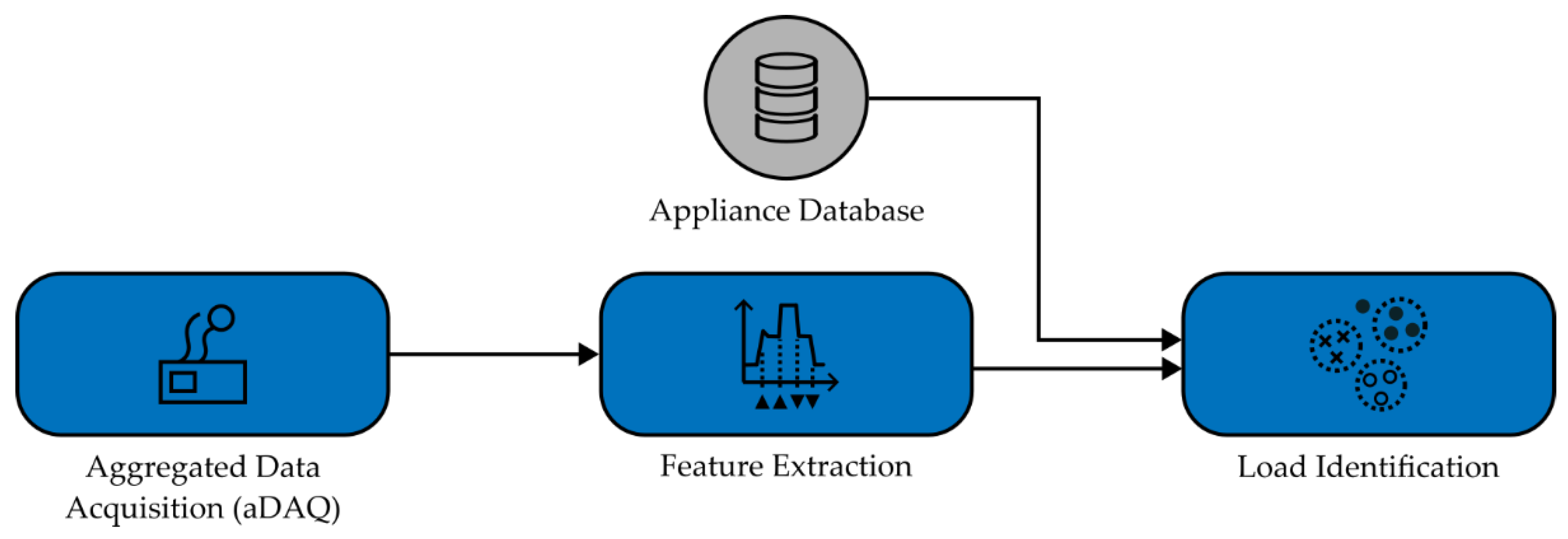
Figure 2.
Illustration of the challenges in event and state definition: Aggregated active power load profile of a projector and a computer with a resolution 5 S/s (a) and the defined appliance states and transients (b), as well as sections of the individual behavior of the projector (c) and the computer (d) with resolutions of 1 S/s and 50 S/s.
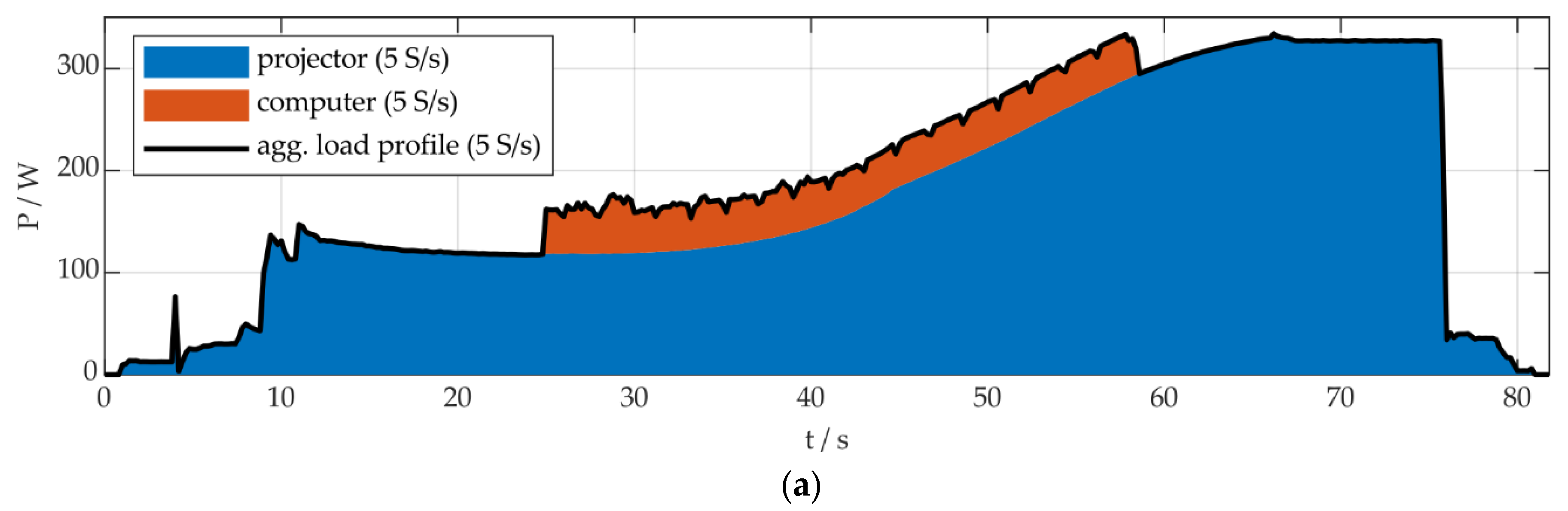
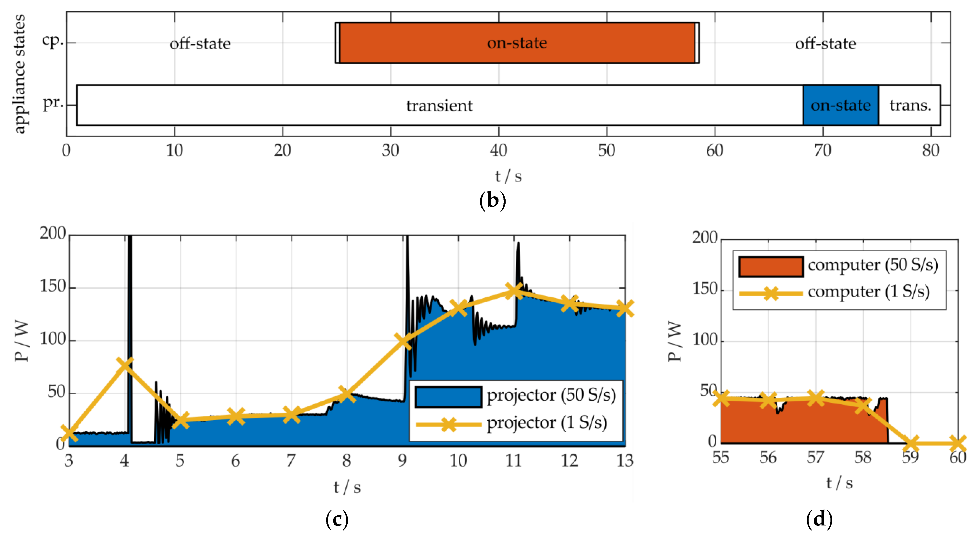
Figure 3.
General NILM methodology for algorithm parametrization, optimization and performance evaluation. Individual appliance data acquisition (iDAQ) is used temporarily, as a ground truth and for building an extended appliance database, for the permanent NILM process. Blue-backgrounded elements are based on aggregated DAQ (aDAQ), iDAQ aspects are marked in orange.
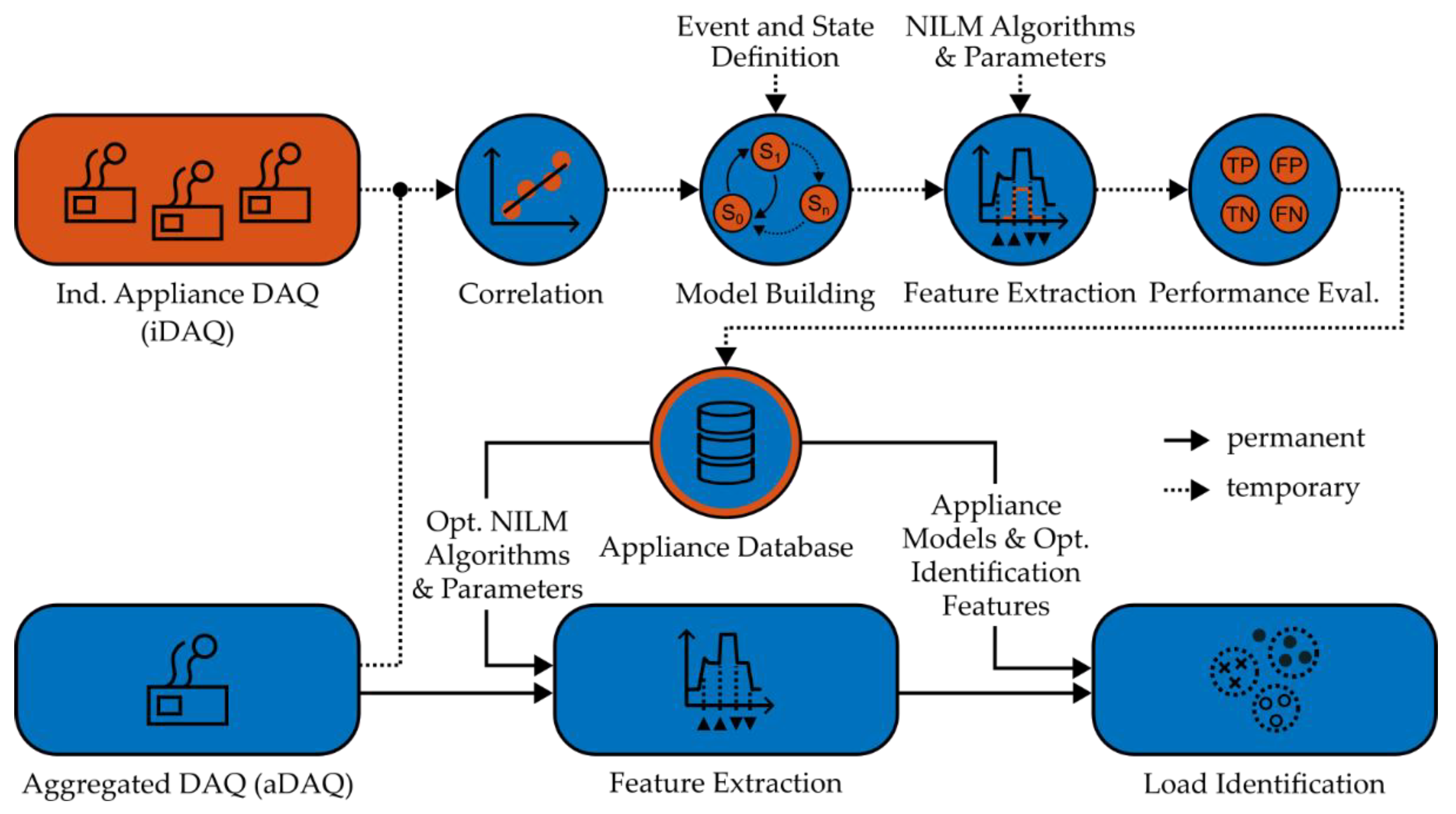
Figure 4.
Illustration of feature extraction for (a) a rising event in active power (P) and (b) a falling event in reactive power (Q).
Figure 4.
Illustration of feature extraction for (a) a rising event in active power (P) and (b) a falling event in reactive power (Q).
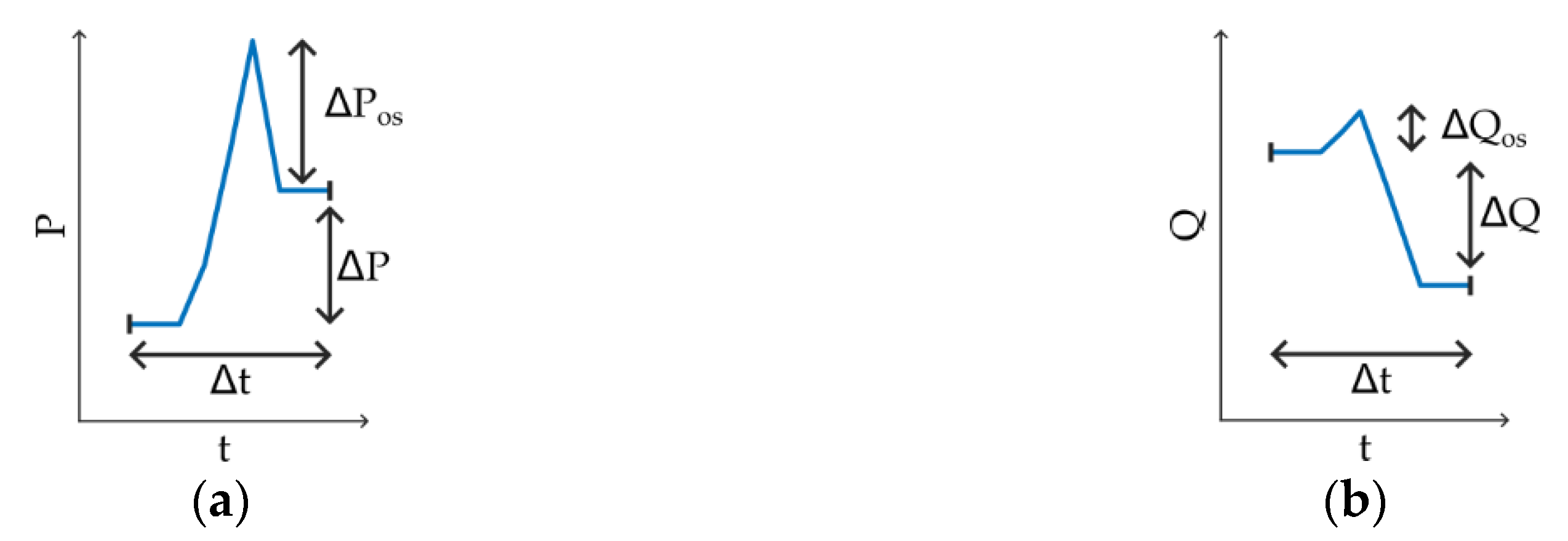
Figure 5.
Appliance database: General methodology.

Figure 6.
Overview of the measurement data: Single-phase active power iDAQ (a), as well as three-phase total active power aDAQ (b) and reactive power aDAQ (c) for time periods of the learning and test data with appliance operation.
Figure 6.
Overview of the measurement data: Single-phase active power iDAQ (a), as well as three-phase total active power aDAQ (b) and reactive power aDAQ (c) for time periods of the learning and test data with appliance operation.
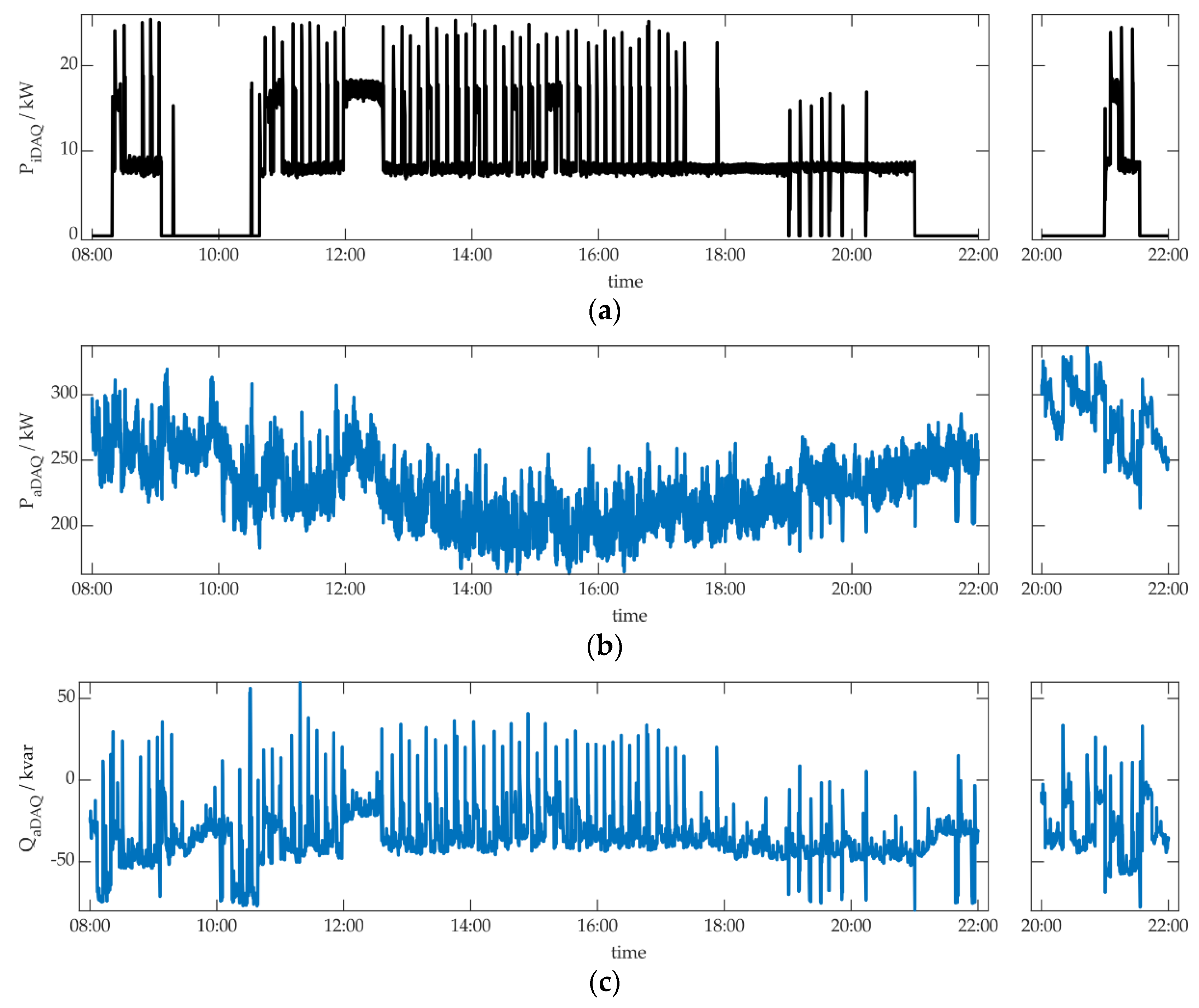
Figure 7.
Selected transients and affiliated steady states, identified using PiDAQ for model building (a), mapped to QiDAQ (b) and all measured aDAQ quantities: PL1,aDAQ (c), QL1,aDAQ (d), PL2,aDAQ (e), QL2,aDAQ (f), PL3,aDAQ (g) and QL3,aDAQ (h).
Figure 7.
Selected transients and affiliated steady states, identified using PiDAQ for model building (a), mapped to QiDAQ (b) and all measured aDAQ quantities: PL1,aDAQ (c), QL1,aDAQ (d), PL2,aDAQ (e), QL2,aDAQ (f), PL3,aDAQ (g) and QL3,aDAQ (h).
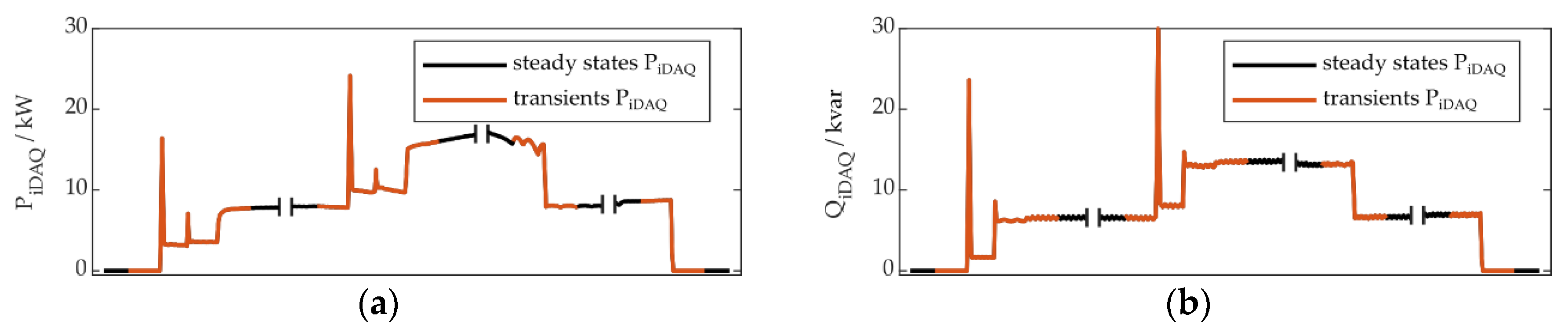
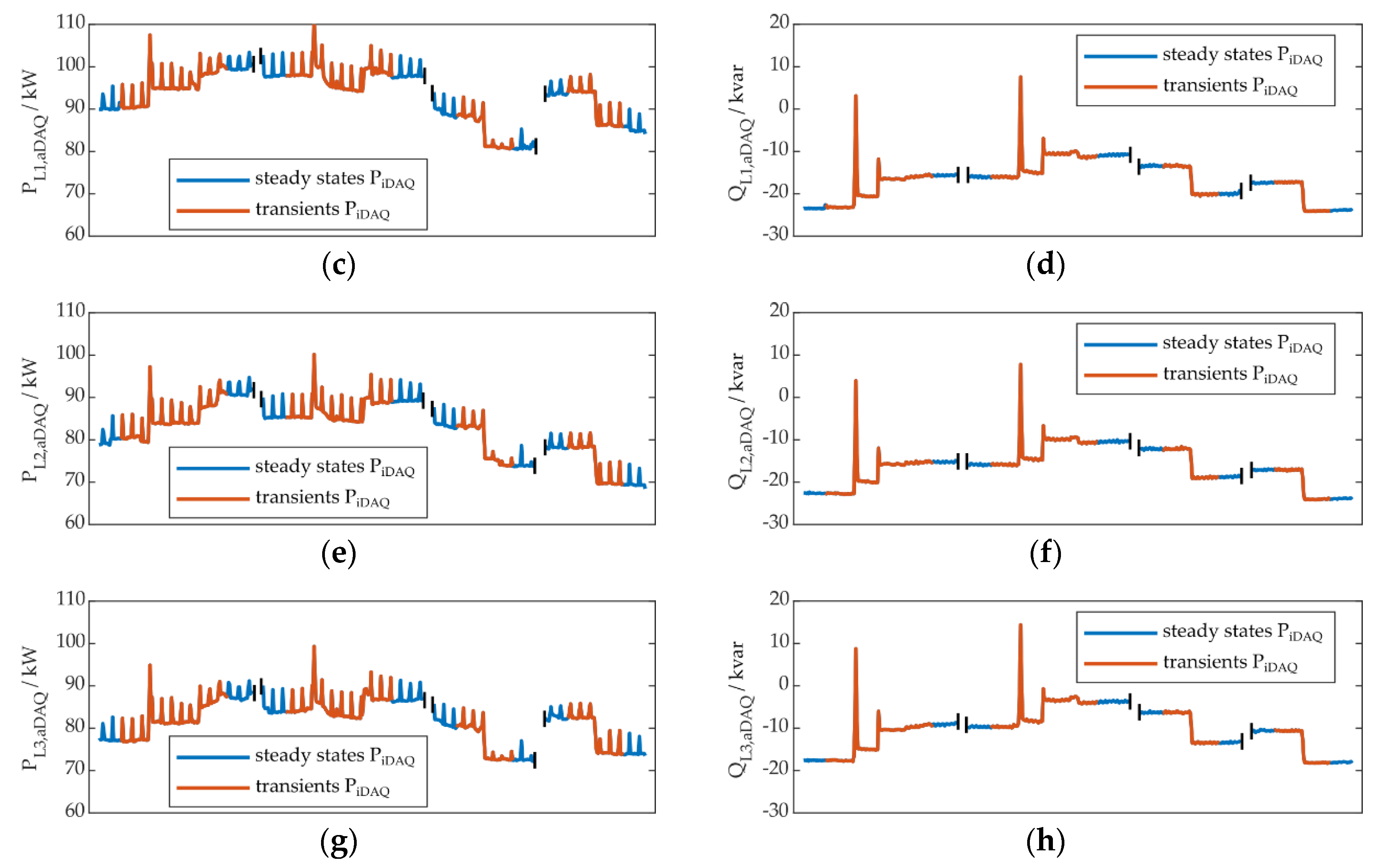
Figure 8.
Appliance model of the refrigeration plant, derived from PiDAQ on the learning day.
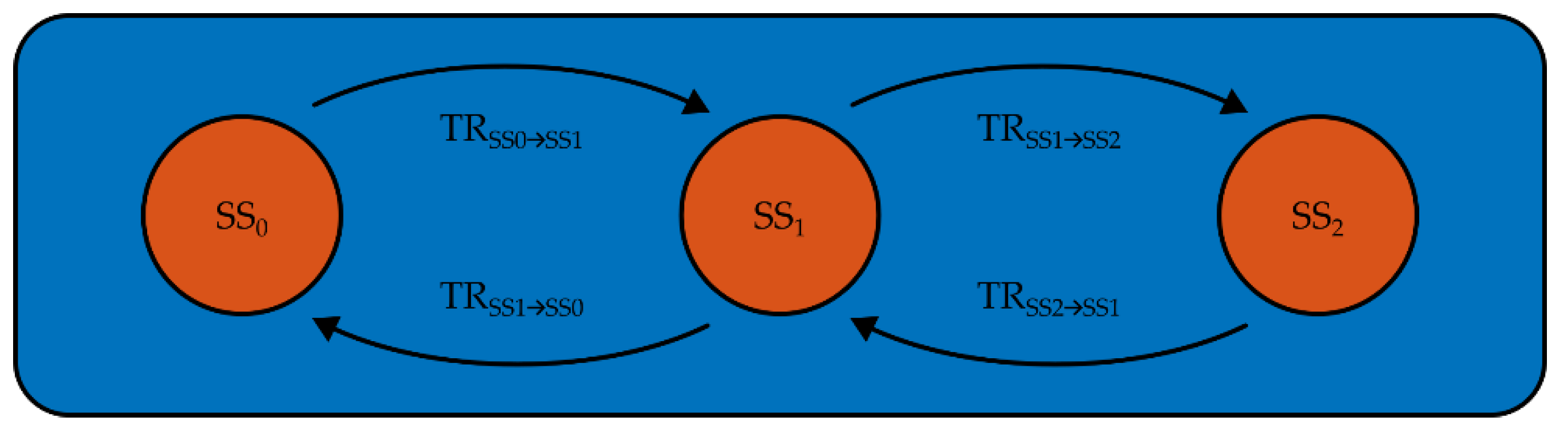
Figure 9.
Illustration of the event detection for one algorithm-parameter-variant: Section of the refrigeration plant’s QiDAQ, containing a transient of the type TRSS1→SS2 (a) and events, detected in this section of QL1,aDAQ (b).
Figure 9.
Illustration of the event detection for one algorithm-parameter-variant: Section of the refrigeration plant’s QiDAQ, containing a transient of the type TRSS1→SS2 (a) and events, detected in this section of QL1,aDAQ (b).
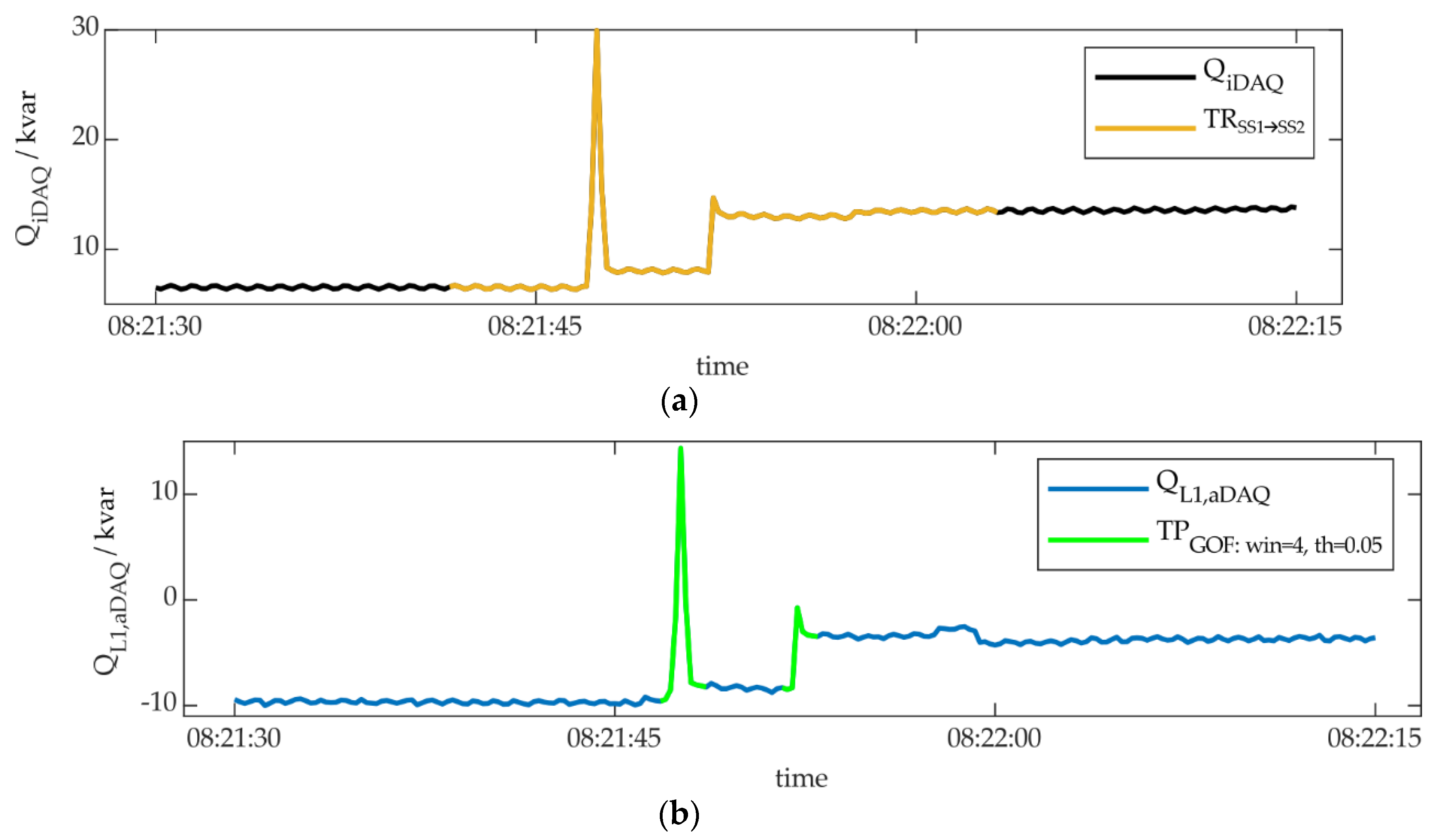
Figure 10.
Clustering of the TP-events, identified by the algorithm χ²-GOF (window size: 4, threshold: 0.05) on the learning day, regarding the features ΔQ and ΔQos (a) and ΔQ and Δt (b).
Figure 10.
Clustering of the TP-events, identified by the algorithm χ²-GOF (window size: 4, threshold: 0.05) on the learning day, regarding the features ΔQ and ΔQos (a) and ΔQ and Δt (b).
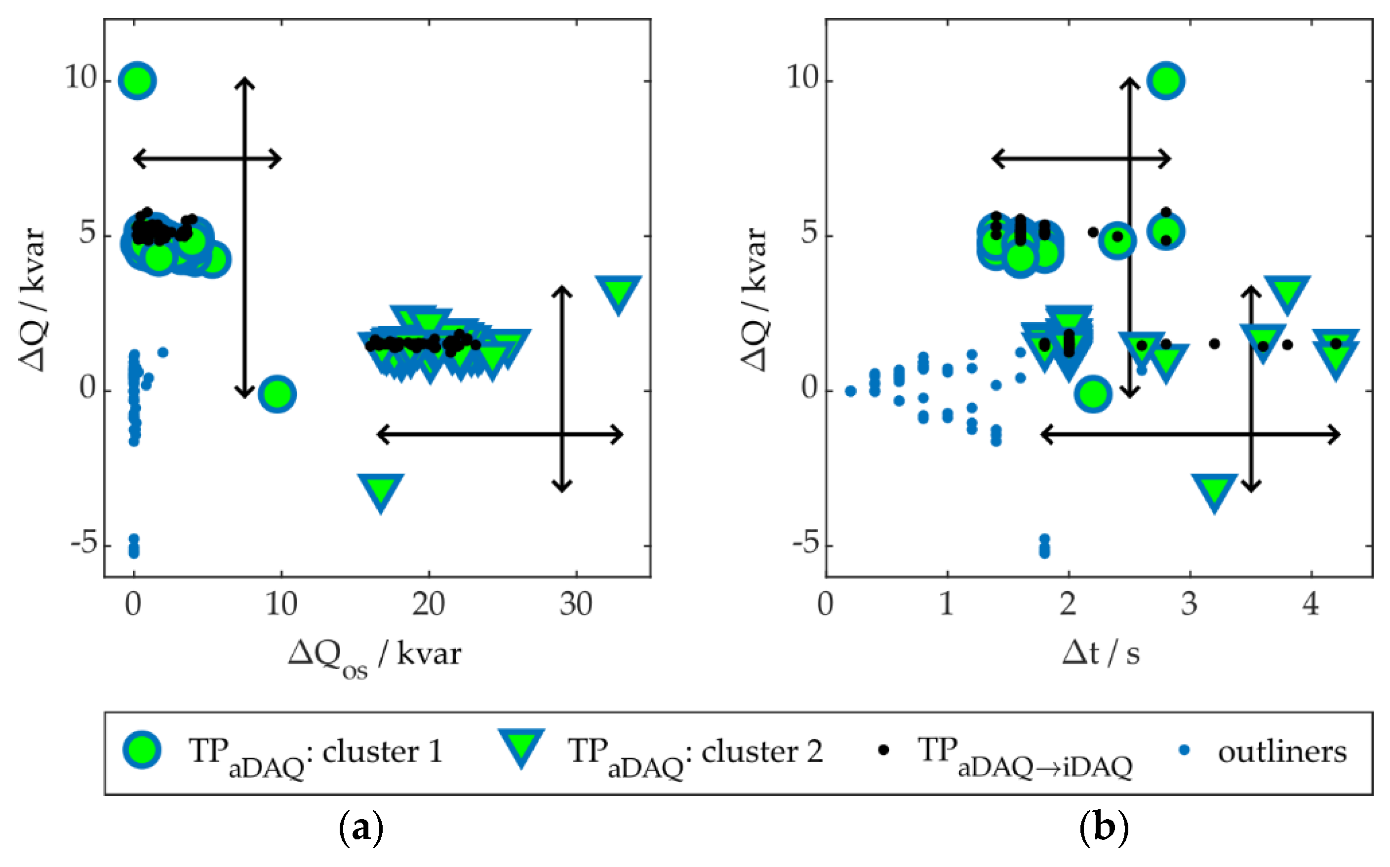
Figure 11.
Illustration of the performance evaluation of one algorithm-parameter-variant, for a section of the learning day: Refrigeration plant’s QiDAQ, including transients of the type TRSS0→SS1 and TRSS1→SS2 (a), as well as the performance of algorithm-parameter-variant i, using QL3,aDAQ (b).
Figure 11.
Illustration of the performance evaluation of one algorithm-parameter-variant, for a section of the learning day: Refrigeration plant’s QiDAQ, including transients of the type TRSS0→SS1 and TRSS1→SS2 (a), as well as the performance of algorithm-parameter-variant i, using QL3,aDAQ (b).
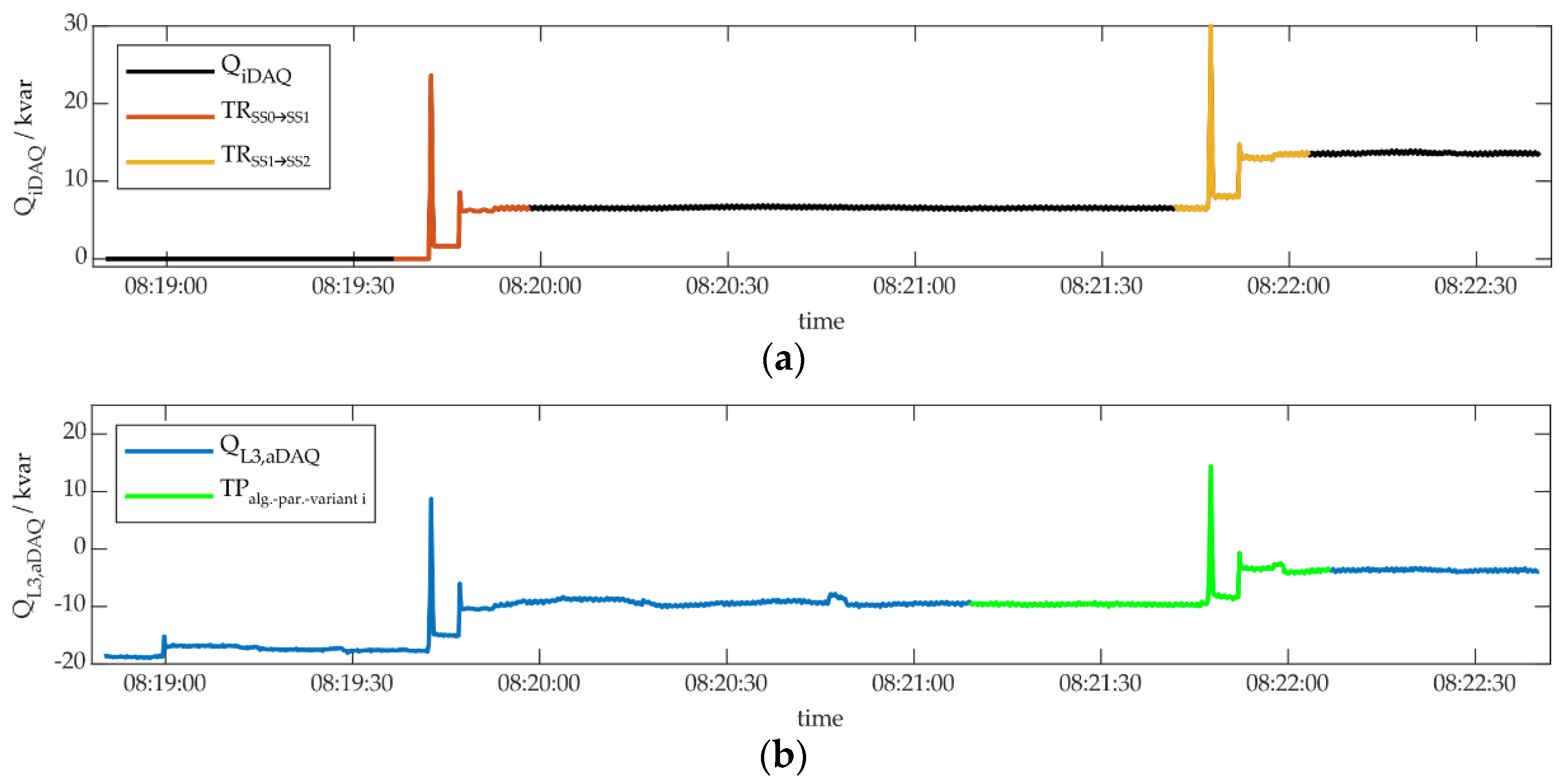
Figure 12.
Illustration of the performance evaluation of two algorithm-parameter-variants, for a section of the learning day: Refrigeration plant’s PiDAQ, including transients of the type TRSS0→SS1 and TRSS1→SS2 (a), as well as the performance of algorithm-parameter-variant j and k, using PL1,aDAQ (b).
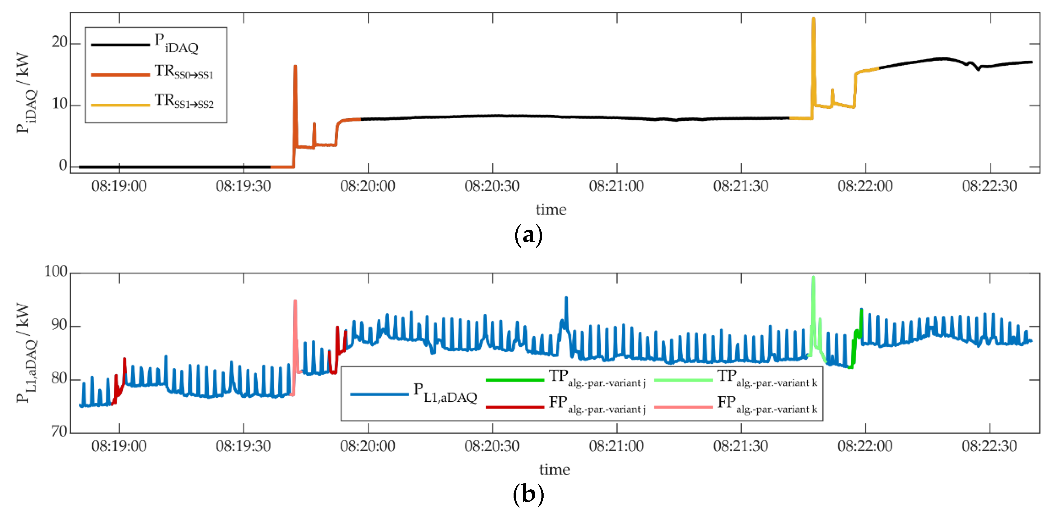
Figure 13.
Results of the algorithm-parameter-variants of the event detection algorithm χ²-GOF for PL3,aDAQ (a) and QL3,aDAQ (b) on the learning day, delivering 100 % TPs, regarding their number of FPs for the transient type TRSS1→SS2 of the refrigeration plant.
Figure 13.
Results of the algorithm-parameter-variants of the event detection algorithm χ²-GOF for PL3,aDAQ (a) and QL3,aDAQ (b) on the learning day, delivering 100 % TPs, regarding their number of FPs for the transient type TRSS1→SS2 of the refrigeration plant.
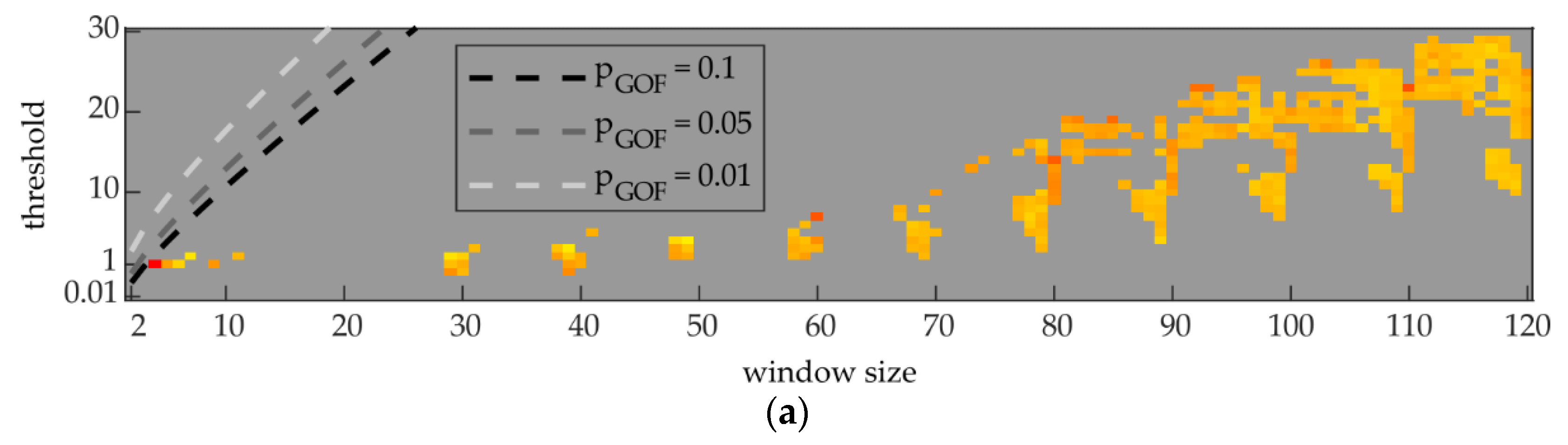
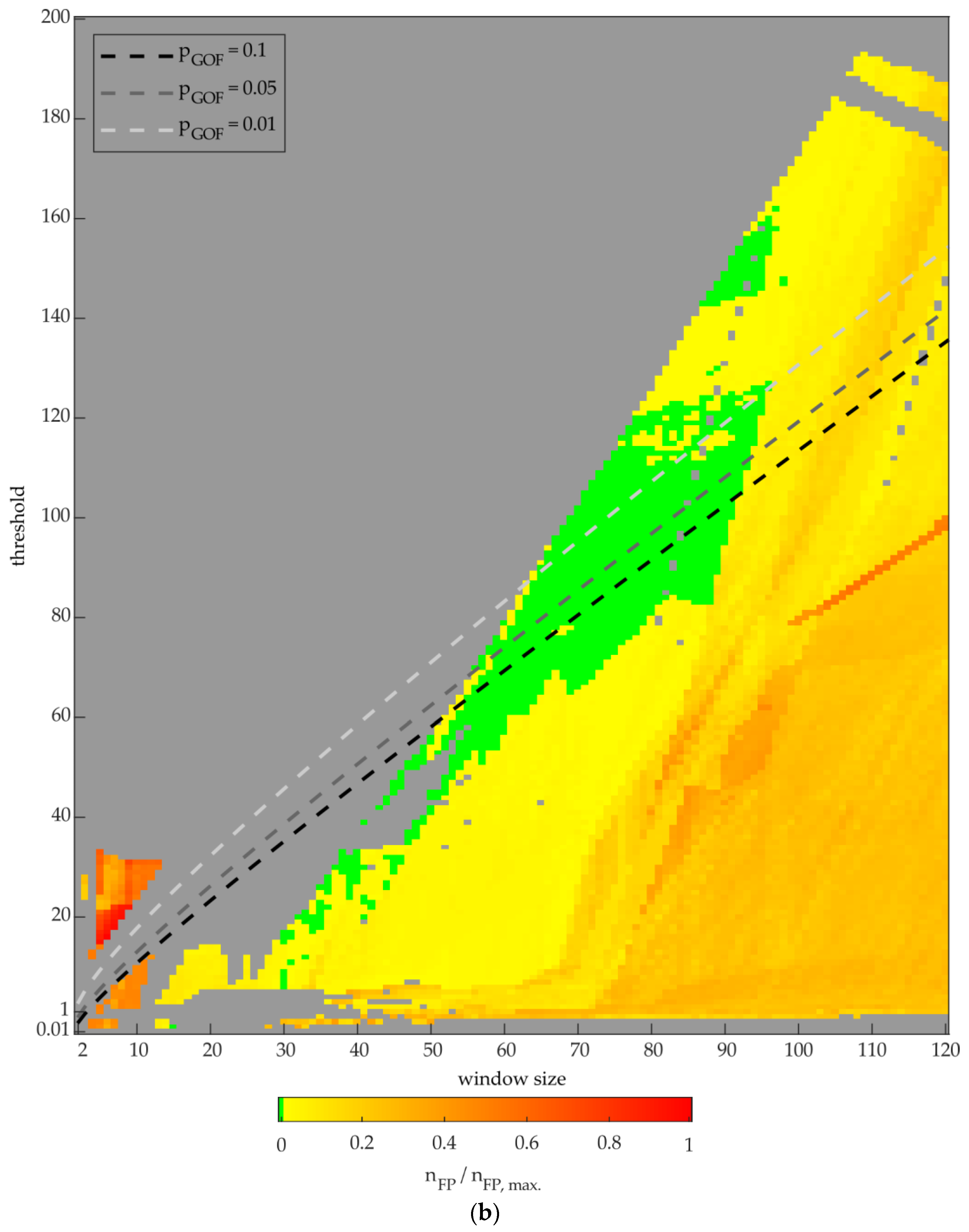
Figure 14.
Results of the algorithm-parameter-variants of the event detection algorithm DSC for PL2,aDAQ (a) and QL2,aDAQ (b) on the learning day, delivering 100 % TPs, regarding their number of FPs for the transient types TRSS1→SS0 and TRSS2→SS1 of the refrigeration plant.
Figure 14.
Results of the algorithm-parameter-variants of the event detection algorithm DSC for PL2,aDAQ (a) and QL2,aDAQ (b) on the learning day, delivering 100 % TPs, regarding their number of FPs for the transient types TRSS1→SS0 and TRSS2→SS1 of the refrigeration plant.
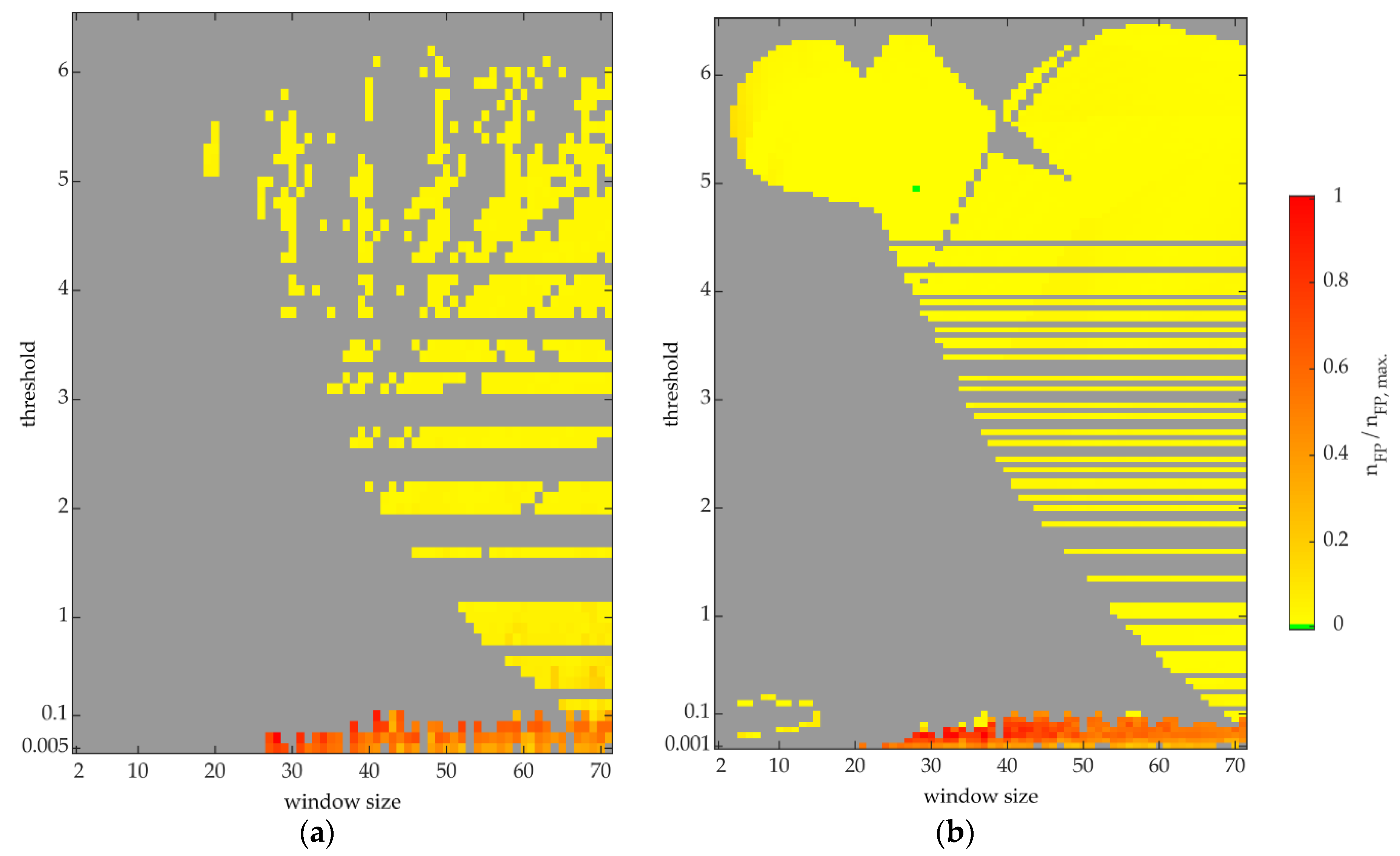
Figure 15.
Load identification results for the transient type TRSS1→SS2 of the refrigeration plant: The building’s PaDAQ, and the detected transients by the applied combination variants for the learning day (a), besides the appliance operation behavior for the learning day (b). The according results for the two test days are displayed in (c) and (d), as well as (e) and (f). All variants show optimal identification results, except for one FP of the P-variant in (e).
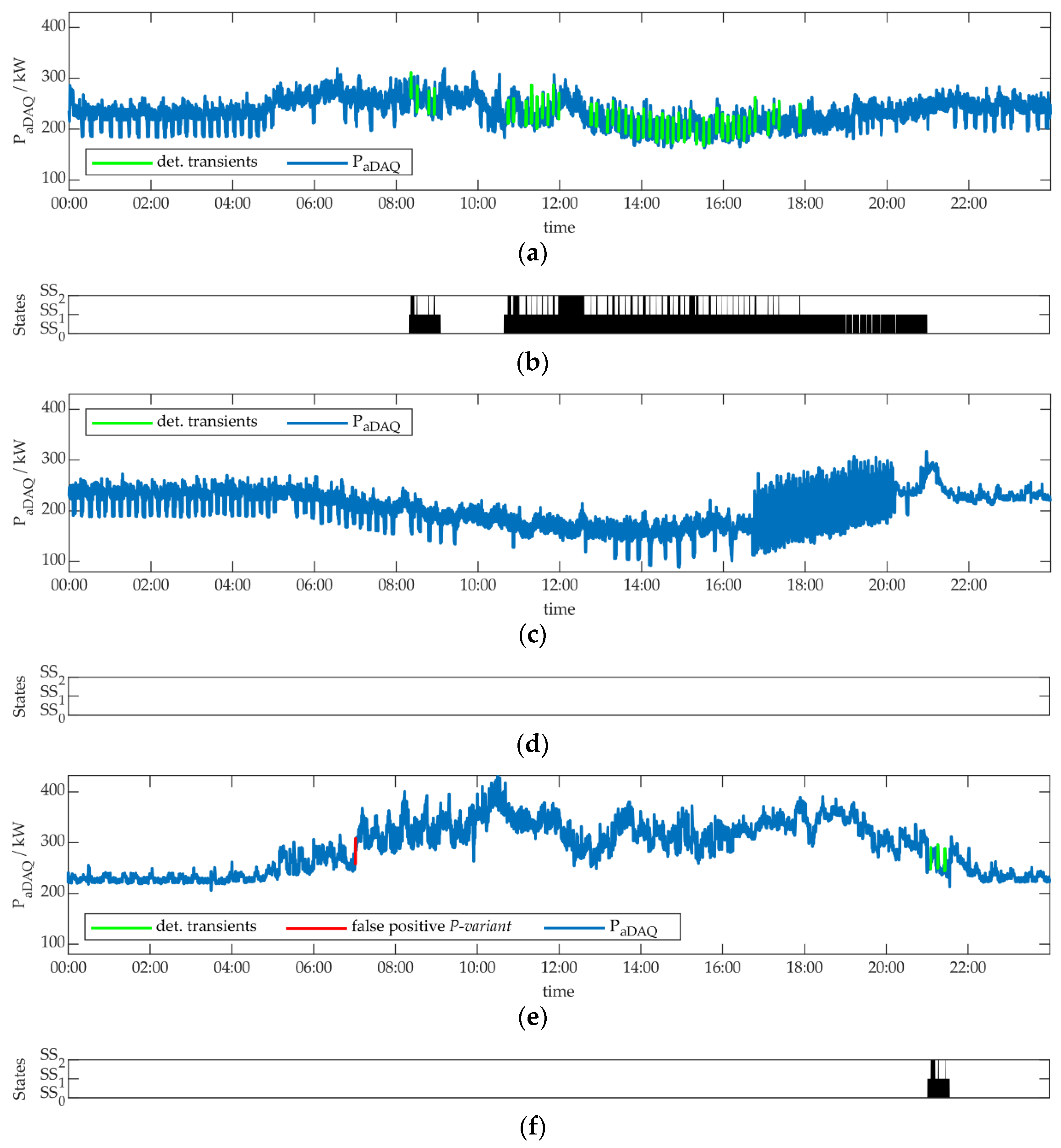
Figure 16.
Load identification results for the transient type TRSS0→SS1 of the refrigeration plant: The building’s PaDAQ, and the detected transients by the applied combination variants for the learning day (a), besides the appliance operation behavior for the learning day (b). The according results for the two test days are displayed in (c) and (d), as well as (e) and (f). All variants show optimal identification results.
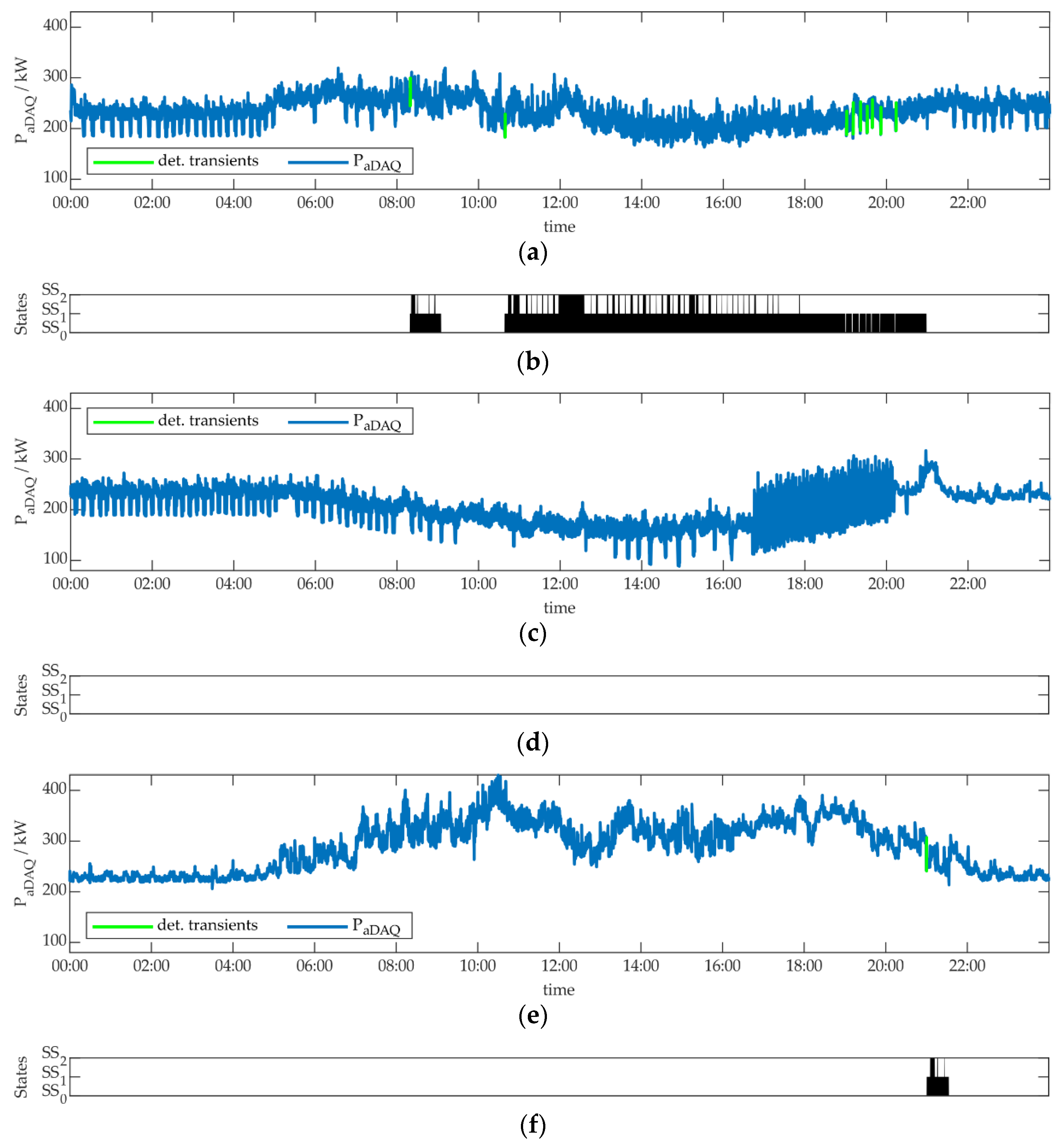
Figure 17.
Load identification results for the transient types TRSS1→SS0 and TRSS2→SS1 of the refrigeration plant: The building’s PaDAQ, and the detected transients by the applied combination variants for the learning day (a), besides the appliance operation behavior for the learning day (b). The according results for the two test days are displayed in (c) and (d), as well as (e) and (f). All variants show optimal identification results.
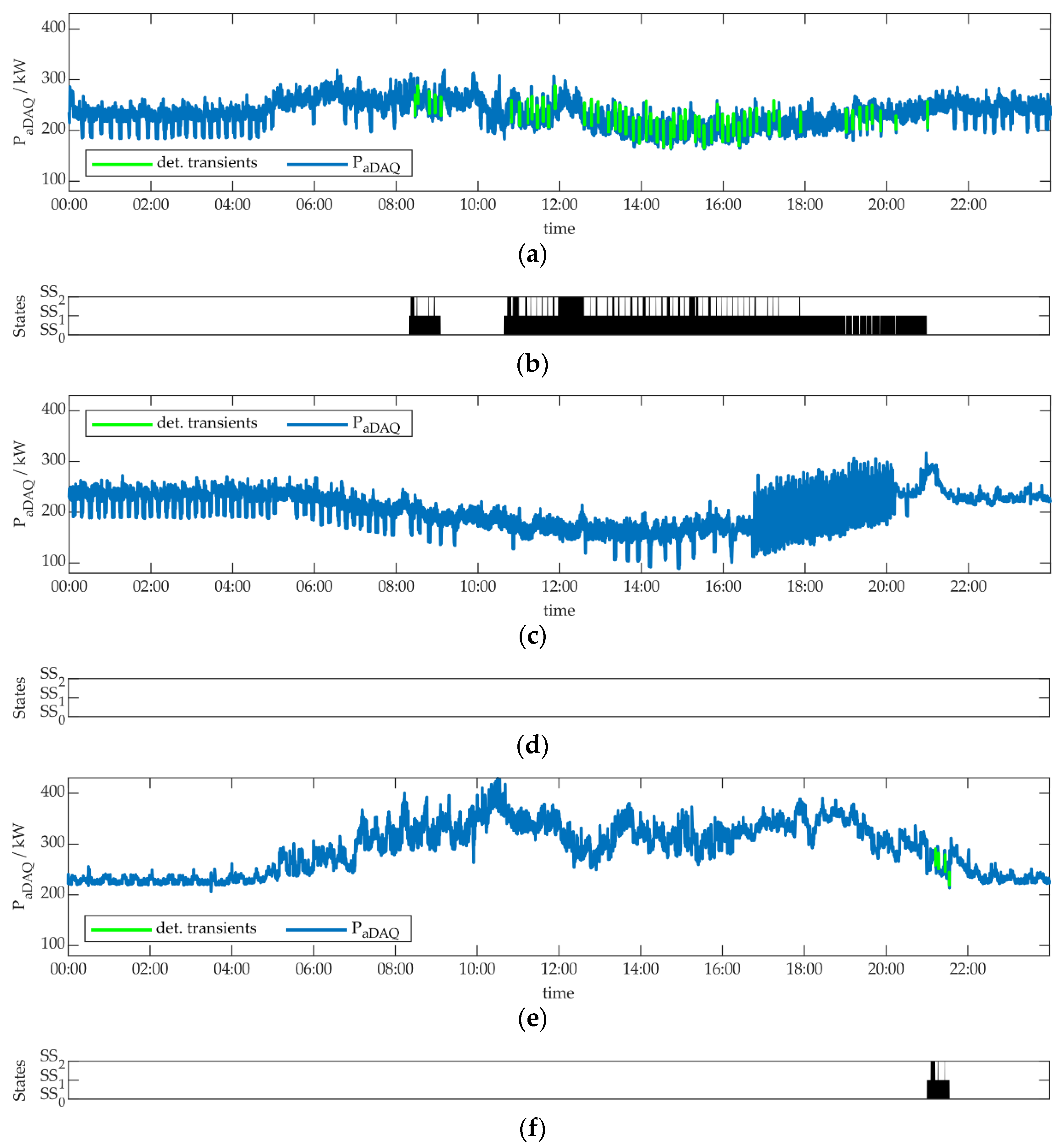

Table 1.
Correlation: General methodology and application in this paper.
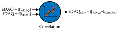 | |
| General methodology: | Application: |
|
|
| Input data: aDAQ and iDAQ, containing individual timestamps each. | |
| Output data: iDAQ, corrected by a potential time shift, relative to aDAQ. | |
Table 2.
Model building: General methodology and application in this paper.
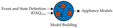 | |
| General methodology: | Application: |
|
|
| Input data: Predefined event and state definition and time-shift corrected iDAQ | |
| Output data: Complete appliance model, based on iDAQ data, containing congruent transient and steady state types | |
Table 3.
Feature extraction: General methodology and application in this paper.
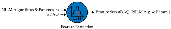 | |
| General methodology: | Application: |
|
|
| Input data: aDAQ data and NILM algorithms, including corresponding parameter sets for these algorithms (applicable for event-based or eventless NILM algorithms) | |
| Output data: aDAQ data feature sets, as a result of the individually applied NILM algorithm-parameter-variants | |
Table 4.
Performance evaluation: General methodology and application in this paper.
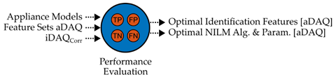 | |
| General methodology: | Application: |
|
|
| Input data: Appliance models, aDAQ feature sets for the applied NILM algorithms and parameter sets, as well as time-shift corrected iDAQ (as ground truth) | |
| Output data: Optimal (combination of) identification features, NILM algorithms and parameters, for the identification of individual appliances’ transient or steady state types | |
Table 5.
Algorithms-parameter-variations, depending on the refrigeration plant’s transient types.
| Algorithm | Parameter | Phase | Transient Type | Win. Size | Threshold |
|---|---|---|---|---|---|
| χ²-GOF | PaDAQ | L1, L2, L3 | TRSS0→SS1, TRSS1→SS2 | 2:120 | 0.01, 0.05, 0.1, 0.5, (1:200) |
| χ²-GOF | PaDAQ | L1, L2, L3 | TRSS1→SS0, TRSS2→SS1 | 2:71 | 0.01, 0.05, 0.1, 0.5, (1:200) |
| χ²-GOF | QaDAQ | L1, L2, L3 | TRSS0→SS1, TRSS1→SS2 | 2:120 | 0.01, 0.05, 0.1, 0.5, (1:200) |
| χ²-GOF | QaDAQ | L1, L2, L3 | TRSS1→SS0, TRSS2→SS1 | 2:71 | 0.01, 0.05, 0.1, 0.5, (1:200) |
| DSC | PaDAQ | L1, L2, L3 | TRSS0→SS1, TRSS1→SS2 | 2:120 | 0.005, 0.01, 0.05, (0.1:0.1:7) |
| DSC | PaDAQ | L1, L2, L3 | TRSS1→SS0, TRSS2→SS1 | 2:71 | 0.005, 0.01, 0.05, (0.1:0.1:7) |
| DSC | QaDAQ | L1, L2, L3 | TRSS0→SS1, TRSS1→SS2 | 2:120 | (0.1, 0.2, 0.5, 1, 2, 5) 10-2, (0.1:0.05:7) |
| DSC | QaDAQ | L1, L2, L3 | TRSS1→SS0, TRSS2→SS1 | 2:71 | (0.1, 0.2, 0.5, 1, 2, 5) 10-2, (0.1:0.05:7) |
Table 6.
Load identification variants for transient type TRSS1→SS2.
| Variant | Algorithm | Parameter | win | th | nTP 1 | nFP 1 | Δ limits 2 | ΔOS limits 2 | Δt limits |
|---|---|---|---|---|---|---|---|---|---|
| Q-variant I | χ²-GOF | QL1,aDAQ | 64 | 96 | 45 | 0 | [5.2, 7.8]. kvar | [11.2, 28.1]. kvar | [10.6, 24.4]. s |
| χ²-GOF | QL2,aDAQ | 88 | 130 | 45 | 0 | [5.5, 8.3]. kvar | [11.1, 28.0]. kvar | [14.2, 32.2]. s | |
| χ²-GOF | QL3,aDAQ | 90 | 146 | 45 | 0 | [6.2, 8.7]. kvar | [9.2, 27.6]. kvar | [9.8, 32.0]. s | |
| Q-variant II | χ²-GOF | QL1,aDAQ | 13 | 0.05 | 45 | 6 | [5.3, 8.2]. kvar | [11.3, 28.2]. kvar | [9.6, 65.6]. s |
| χ²-GOF | QL2,aDAQ | 18 | 0.05 | 45 | 4 | [1.3, 8.5]. kvar | [11.2, 28.1]. kvar | [12.0, 96.4]. s | |
| χ²-GOF | QL3,aDAQ | 15 | 0.05 | 45 | 0 | [5.4,8.9]. kvar | [9.2, 28.2]. kvar | [10.4, 58.0]. s | |
| P-variant | χ²-GOF | Combination of 830 algorithm-parameter-variants using PaDAQ, see text. | |||||||
1 Learning day performance. 2 Rounded to 1 decimal point.
Table 7.
Load identification variants for transient type TRSS0→SS1.
| Variant | Algorithm | Parameter | win | th | nTP 1 | nFP 1 | Δ limits 2 | ΔOS limits 2 | Δt limits |
|---|---|---|---|---|---|---|---|---|---|
| PQ-variant (short) | χ²-GOF | PL1,aDAQ | 4 | 4 | 9 | 44 | [4.4, 16.7]. kW | [0.0, 15.0]. kW | [0.6, 1.6]. s |
| χ²-GOF | PL2,aDAQ | 6 | 6 | 9 | 48 | [0.0, 17.7]. kW | [0.0, 9.4]. kW | [0.2, 1.6]. s | |
| χ²-GOF | PL3,aDAQ | 4 | 6 | 9 | 43 | [5.9, 18.4]. kW | [0.0, 13.5]. kW | [0.4, 1.2]. s | |
| χ²-GOF | QL1,aDAQ | 3 | 54 | 9 | 44 | [9.5, 25.7]. kvar | [0.0, 15.1]. kvar | [0.6, 0.8]. s | |
| χ²-GOF | QL2,aDAQ | 3 | 85 | 9 | 12 | [20.0, 26.6]. kvar | [0.0, 0.0]. kvar | [0.4, 0.8]. s | |
| χ²-GOF | QL3,aDAQ | 2 | 42 | 9 | 17 | [10.0, 19.8]. kvar | [0.0, 10.8]. kvar | [0.4, 0.6]. s |
1 Learning day performance. 2 Rounded to 1 decimal point.
Table 8.
Load identification variants for transient type TRSS1→SS0 and TRSS2→SS1 together.
| Variant | Algorithm | Parameter | win | th | nTP 1 | nFP 1 | Δ limits 2 | ΔOS limits 2 | Δt limits |
|---|---|---|---|---|---|---|---|---|---|
| DSC-variant | DSC | PL1,aDAQ | 62 | 2.6 | 54 | 51 | [-19.4, -7.4]. kW | [0.0, 9.8]. kW | [10.6, 25.0]. s |
| DSC | PL2,aDAQ | 53 | 2.2 | 54 | 42 | [-18.9, -8.3]. kW | [0.0, 9.9]. kW | [11.8, 21.0]. s | |
| DSC | PL3,aDAQ | 54 | 3 | 54 | 59 | [-19.2, -7.2]. kW | [0.1, 8.1]. kW | [9.2, 18.0]. s | |
| DSC | QL2,aDAQ | 28 | 4.95 | 54 | 0 | [-7.4, -6.1]. kvar | [0.0, 6.4]. kvar | [2.6, 4.2]. s |
1 Learning day performance. 2 Rounded to 1 decimal point.
Disclaimer/Publisher’s Note: The statements, opinions and data contained in all publications are solely those of the individual author(s) and contributor(s) and not of MDPI and/or the editor(s). MDPI and/or the editor(s) disclaim responsibility for any injury to people or property resulting from any ideas, methods, instructions or products referred to in the content. |
(c) 2025 by the authors. Licensee MDPI, Basel, Switzerland. This article is an open access article distributed under the terms and conditions of the Creative Commons Attribution (CC BY) license (https://creativecommons.org/licenses/by/4.0/).
Copyright: This open access article is published under a Creative Commons CC BY 4.0 license, which permit the free download, distribution, and reuse, provided that the author and preprint are cited in any reuse.


