
Submitted:
19 December 2024
Posted:
23 December 2024
You are already at the latest version
Abstract
In this article, we propose a new distribution based on the convolution of two independent Akash (AK) random variables with the same parameter, which we call the Akash convolution (AKC) distribution. We study its density and some basic properties, and perform parameter estimation using the methods of moments and maximum likelihood (ML), along with the Fisher information. We evaluate the performance of the ML estimator through a simulation study. Additionally, we present two applications with real data, demonstrating a better performance of the AKC distribution compared to two other distributions.
Keywords:
Akash distribution
; Convolution
; Maximum likelihood
MSC: 62E99; 62P99; 62F10
1. Introduction
A widely used distribution is the Lindley model (see Lindley [1]), we say that a random variable X has a Lindley distribution (L) if its probability density function (pdf) is given by
where is a shape parameter. We denote this by . The cumulative distribution function (cdf) corresponding to (1) is
The L distribution has been used in various settings such as engineering, demography, reliability, and medicine, among others. Some researchers who have carried out these studies are: Hussain [2], Ghitany et al. [3], Zakerzadeh and Dolati [4], Gómez-Déniz and Calderin-Ojeda [5], Krishna and Kumar [6], Bakouch et al. [7], Shanker et al. [8], Ghitany et al. [9], Al-Mutairi et al. [10], Oluyede and Yang [11], Shanker et al. [12] and Abouammoh et al. [13], among others.
Shanker [14] introduced the Akash distribution and applied it to real lifetime data sets from medical science and engineering. Thus we say that a random variable Y has an Akash distribution (AK) with shape parameter if its pdf is given by
where is a shape parameter, and it is denoted by .
In Figure 1, we show the pdf of the distribution for several values of .
Some properties of this pdf are:
- a)
- The cdf of Y is
- b)
- For the r-th moment of Y is
- c)
- The moment generating function () is given by
Extensions distribution are given by Shanker and Shukla [15], Shanker and Shukla [16] and Gómez et al. [17], among others.
In this article, we consider two independent random variables with the same parameter and study their convolution. We show that the convolution distribution has a closed form and several interesting properties. Applications show that it can be an alternative to the and L distributions.
The paper develops as follows: In Section 2, we furnish the distribution and its properties. In Section 3, we perform inference by the methods of moments and maximum likelihood; the Fisher information is obtained, and a simulation study is also carried out. In Section 4, applications are made to two real data sets and compared with the and L distributions. In Section 5, we provide some conclusions.
2. AKC Distribution
In this section we introduce the density function properties of the distribution.
2.1. Density Function
Definition 1.
We say that a random variable Z has a distribution with shape parameter θ, , if it has the following pdf:
where .
In Figure 2, we show the pdf of the distribution for several values of .
2.2. Properties
The following proposition shows that the pdf of the distribution can be obtained from a convolution of two distributions.
Proposition 1.
Let , be two independent random variables and define , then .
Proof.
Since and are independent, the pdf of Z may be obtained from the following convolution product: for ,
By calculating the right-side integral, the result follows. □
The following proposition shows the cdf of the distribution.
Proposition 2.
Let . Then, the cdf of Z is given by
where and is the incomplete gamma function.
Proof.
By directly calculating the cdf of Z we have
and making the following change of variable: , the result is obtained. □
2.3. Reliability Analysis
The reliability function and the hazard function of the distribution are given in the following corollary.
Corollary 1.
Let . Then, the and of T are given by
where .
In Figure 3, we show the hazard function of AKC distribution for several values of .
Proposition 3.
Let . Then, the hazard function of T is increasing for all .
2.4. Order Statistics
Let be a random sample of a random variable . Let us denote by the order statistics, .
Proposition 4.
The pdf of is
where and In particular, the pdf of the minimum, , is
and the pdf of the maximum, , is
Proof.
Since we are dealing with an absolutely continuous model, the pdf of the order statistic is obtained by applying
where F and f denote the cdf and pdf of the parent distribution, in this case. □
2.5. Moments
In this subsection we provide the moments, the moment generating function and skewness and kurtosis coefficients.
Proposition 5.
Let . Then, for the r-moment of Z is given by
Proof.
Using the representation of Z given in Proposition 1 and the binomial theorem, we have that the r-th moment is
then using the moments of the random variable given in (5), the result is obtained. □
Proposition 6.
Let . Then, the moment generating function of the random variable Z is given by
Proof.
Using the representation given in Proposition 1, we get:
and using the moment generating function of the random variable given in (6), the result follows. □
Corollary 2.
Let . Then, the mean and variance Z are given respectively by:
The skewness and kurtosis coefficients are respectively:
Figure 4 depicts plots of skewness and kurtosis coefficients of the distribution.
3. Inference
In this section we estimate the parameter of the model using the method of moments (MM) and the method of maximum likelihood (ML). Asymptotic properties of the ML estimator are discussed and a simulation study is presented.
3.1. Method of Moments
Let be a random sample from . Let be the first sample moment.
Proposition 7.
Given , a random sample from , the method of moment estimator of θ () provides the following estimator:
Proof.
The equation for the method of moments is given by
Solving equation (11) for the parameter , we obtain the result. □
3.2. Maximum Likelihood Estimation
For a random sample, , derived from the ) distribution, the log-likelihood function can be written as
The score equation are given by
so we get this equation
The ML estimator for () is obtained by solving equation (13). Note that this equation is identical to the equation derived for the method of moments. Consequently, the ML estimator of coincides with the moments estimator given in the Proposition 7.
Hence, for large samples, the ML estimator, , is asymptotically normal. That is,
where the asymptotic variance of the ML estimator is the inverse of Fisher’s information:
3.3. Simulation Study
To examine the performance of the ML estimator of the parameter of the distribution, a simulation study is carried out. An algorithm is available to generate random numbers from the distribution. The simulation analysis is performed generating 1000 samples of sizes 50 and 100 from the distribution. The algorithm used to generate random numbers from the distribution is shown below. The Algorithm 1 is based on the representation given in Proposition 1.
| Algorithm 1:for simulating from the can proceed as follows. |
|
Table 1 shows the empirical bias (B), the average of the standard errors (SE), the empirical root mean squared error (RMSE) and the coverage probability (CP). It is to be noted that the CP converge reasonably well to the nominal value used in their construction (95%), suggesting that the normal distribution is a reasonable asymptotic distribution for the the ML estimators in the AKC model. Also, Table 1 shows that, the performance of the estimates is very good even when n is small.
4. Applications
In this Section the distribution is fitted to two engineering science data sets and compared with the and L distributions.
4.1. Application 1
In this application the data set consists of the strength of glass of the aircraft window reported by Fuller et al. [19]. The data are shown in Table 2.
Descriptive statistics are given in Table 3, where CS is the sample skewness coefficient and CK is the sample kurtosis coefficient.
Table 4 shows the ML estimates of the parameters of the , and L models together with their standard errors in parentheses, Also the values of the AIC and BIC criteria are given for each model, (Akaike information criterion (AIC) introduced by Akaike [20] and the Bayesian information criterion (BIC) proposed by Schwarz [21]).
Observe that the smallest AIC and BIC values correspond to the AKC model, meaning that this model produces a better fit than the and L models.
For the fitted distribution we calculated the quantile residuals (QR). If the model is appropriate for the data, the QRs should be a sample from the standard normal model (see Dunn and Smyth [22]). This assumption can be validated with traditional normality tests, such as the Anderson-Darling (AD), Cramèr-von Mises (CVM) and Shapiro-Wilkes (SW) tests.
In Figure 5 the QRs for the AKC distribution are shown together with the p-values of the AD, CVM and SW normality tests. It is seen that the AKC distribution verifies the assumption that the QRs come from the standard normal distribution, validating the fit of the distribution to the strength of glass data.
4.2. Application 2
In this application we model a data set collected by the Department of Mines of the University of Atacama, Chile. The data, consisting of Yttrium measurements in 86 samples of mineral, are shown in Table 5.
Summary statistics are reported in Table 6. ML estimates of the parameter of the , and L models, together with their SE and the values of the AIC and BIC are given in Table 7.
We observe that the smallest values of the AIC and BIC criteria correspond to the AKC model, meaning that the AKC model fits the data better than the AK and L models.
The residual quantiles of the distribution are shown in Figure 6. Also the p-values for the AD, CVM and SW normality tests are given to verify if the QRs come from a standard normal distribution. These indicate that the distribution provides a good fit for the Yttrium data.
5. Conclusions
In this article, we have studied the convolution of two independent random variables with a parameter in common. We have given some of the properties of the new distribution and developed parameter estimates by the methods of moments and maximum likelihood. A simulation study is carried out to investigate the performance of the ML estimator. Also, the ability of the distribution is demonstrated in two applications made to real data sets. It consistently produces better fits than the and L distributions.
Some additional features of the are:
- The distribution has a simple representation.
- The cumulative distribution and risk functions are explicit and represented by known functions.
- The Moments and Maximum Likelihood estimators coincide and have closed form solutions.
- The Maximun Likelihood estimator performs very well, even when samples are small.
- Applications show that the distribution is a good alternative to model positively skewed data when kurtosis is not too high. This is confirmed by the AIC and BIC model selection criteria and statistical tests such as Anderson-Darling, Cramèr-von Mises and Shapiro-Wilkes.
Author Contributions
Conceptualization, L.F-L. and N.M.O.; methodology, H.W.G.; software, L.F-L. and H.W.G.; validation, O.V., N.M.O. and H.W.G.; formal analysis, N.M.O. and H.W.G.; investigation, L.F-L. and O.V.; writing—original draft preparation, L.F-L. and N.M.O.; writing—review and editing, L.F-L. and O.V.; funding acquisition, L.F-L. and H.W.G. All authors have read and agreed to the published version of the manuscript.
Funding
This research received no external funding
Institutional Review Board Statement
Not applicable.
Informed Consent Statement
Not applicable.
Data Availability Statement
The data used in this paper are contained in the text, specifically in Tables 2 and 5.
Conflicts of Interest
The authors declare no conflict of interest.
References
- Lindley, D.V. Fiducial distributions and Bayes’ theorem. J. R. Stat. Soc. Ser. B 1958, 20, 102–107. [Google Scholar] [CrossRef]
- Hussain, E. The non-linear functions of Order Statistics and Their Properties in selected probability models, Ph.D thesis, Department of Statistics, University of Karachi, Pakistan, 2006.
- Ghitany, M.E.; Atieh, B.; Nadarajah, S. Lindley distribution and its applications. Math. Comput. Simul. 2008, 78(4), 493–506. [Google Scholar] [CrossRef]
- Zakerzadeh, H.; Dolati, A. Generalized Lindley distribution. J. Math. Ext. 2009, 3(2), 13–25. [Google Scholar]
- Gómez-Déniz, E.; Calderin-Ojeda, E. The discrete Lindley distribution: properties and application, J. Stat. Comput. Simul. 2011, 81(11), 1405–1416. [Google Scholar] [CrossRef]
- Krishna, H.; Kumar, K. Reliability estimation in Lindley distribution with progressively type II right censored sample. Math. Comput. Simulat. 2011, 82(2), 281–294. [Google Scholar] [CrossRef]
- Bakouch, H.S.; Al-Zaharani, B.; Al-Shomrani, A.; Marchi, V.; Louzada, F. An extended Lindley distribution. J. Korean Stat. Soc. 2012, 41, 75–85. [Google Scholar] [CrossRef]
- Shanker, R.; Sharma, S.; Shanker, R. A two-parameter Lindley distribution for modeling waiting and survival times data. Appl. Math. 2013, 4, 363–368. [Google Scholar] [CrossRef]
- Ghitany, M.; Al-Mutairi, D.; Balakrishnan, N.; Al-Enezi, I. Power Lindley distribution and associated inference. Comput. Stat. Data Anal. 2013, 64, 20–33. [Google Scholar] [CrossRef]
- Al-Mutairi, D.K.; Ghitany, M.E.; Kundu, D. Inferences on stress-strength reliability from Lindley distributions. Commun. Stat. – Theory Methods 2013, 42, 1443–1463. [Google Scholar] [CrossRef]
- Oluyede, B.O.; Yang, T. A new class of generalized Lindley distribution with applications. J. Stat. Comput. Simul. 2014, 85(10), 2072–2100. [Google Scholar] [CrossRef]
- Shanker, R.; Hagos, F.; Sujatha, S. On modeling of Lifetimes data using exponential and Lindley distributions. Biom. Biostat. Int. J. 2015, 2(5), 1–9. [Google Scholar] [CrossRef]
- Abouammoh, A.M.; Alshangiti, A.M.; Ragab, I.E. A new generalized Lindley distribution. J. Stat. Comput. Simul. 2015, 85(18), 3662–3678. [Google Scholar] [CrossRef]
- Shanker, R. Akash Distribution and Its Applications. International Journal of Probability and Statistics 2015, 4(3), 65–75. [Google Scholar]
- Shanker, R.; Shukla, K.K. On Two-Parameter Akash Distribution. Biom. Biostat. Int. J. 2017, 6(5), 00178. [Google Scholar] [CrossRef]
- Shanker, R.; Shukla, K.K. Power Akash Distribution and Its Application. J. Appl. Quant. Methods 2017, 12(3), 1–10. [Google Scholar]
- Gómez, Y.M.; Firinguetti-Limone, L.; Gallardo, D.I.; Gómez, H.W. An Extension of the Akash Distribution: Properties, Inference and Application. Mathematics 2014, 12, 31. [Google Scholar] [CrossRef]
- Glaser, R.E. Bathtub and Related Failure Rate Characterizations. J. Am. Stat. Assoc. 1980, 75(371), 667–672. [Google Scholar] [CrossRef]
- Fuller, E.J.; Frieman, S.; Quinn, J.; Quinn, G.; Carter, W. Fracture mechanics approach to the design of glass aircraft windows: A case study, SPIE Procceding, 1994, Vol. 2286, 419–430. [CrossRef]
- Akaike, H. A new look at the statistical model identification. IEEE Trans. Automat. Contr. 1974, 19, 716–723. [Google Scholar] [CrossRef]
- Schwarz, G. Estimating the dimension of a model. Ann. Stat. 1978, 6, 461–464. [Google Scholar] [CrossRef]
- Dunn, P.K.; Smyth, G.K. Randomized Quantile Residuals. J. Comput. Graph. Stat. 1996, 5(3), 236–244. [Google Scholar] [CrossRef]
Figure 1.
Examples of the 0.6) (black color), 0.8) (blue color) and 1.2) (red color).
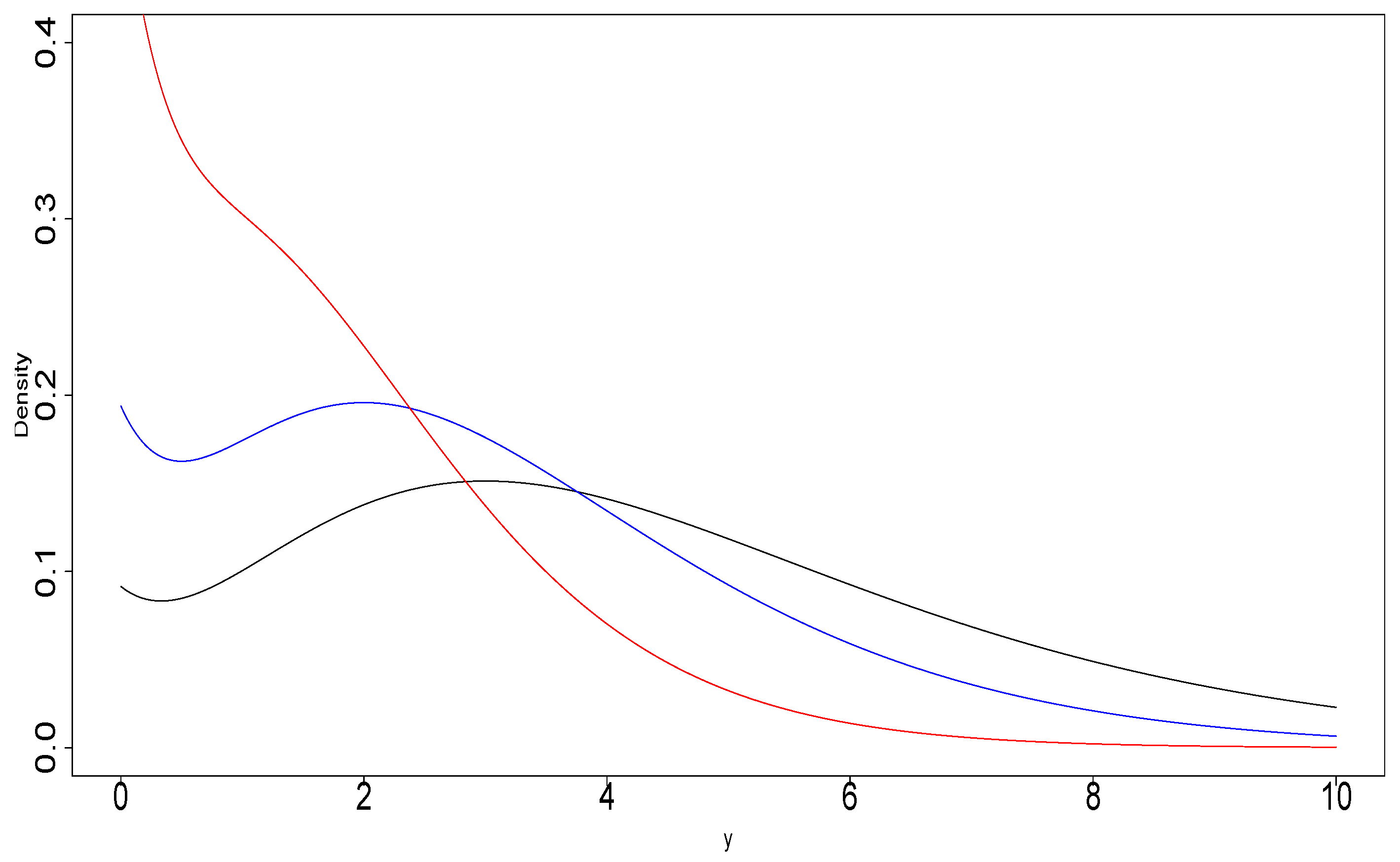
Figure 2.
Examples of the 0.6) (black color), 0.8) (blue color) and 1.2) (red color).
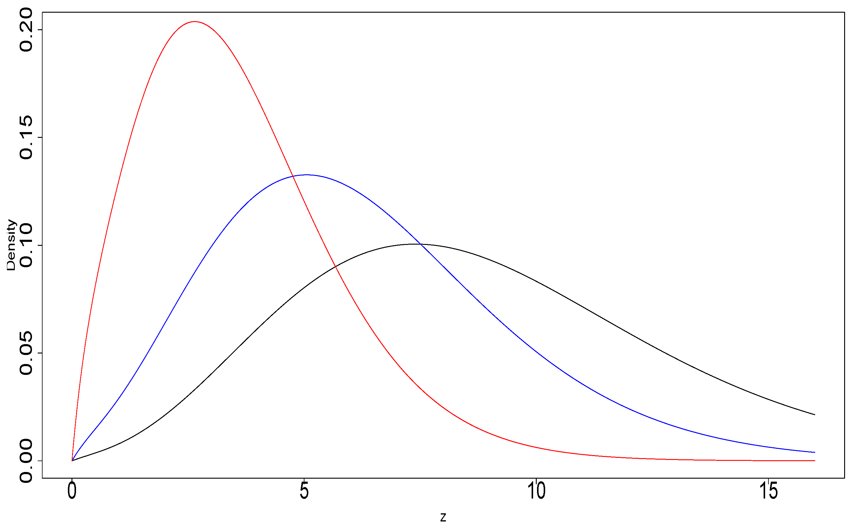
Figure 3.
Hazard function of AKC distribution for selected values of : (black color), (blue color) and (red color)
Figure 3.
Hazard function of AKC distribution for selected values of : (black color), (blue color) and (red color)
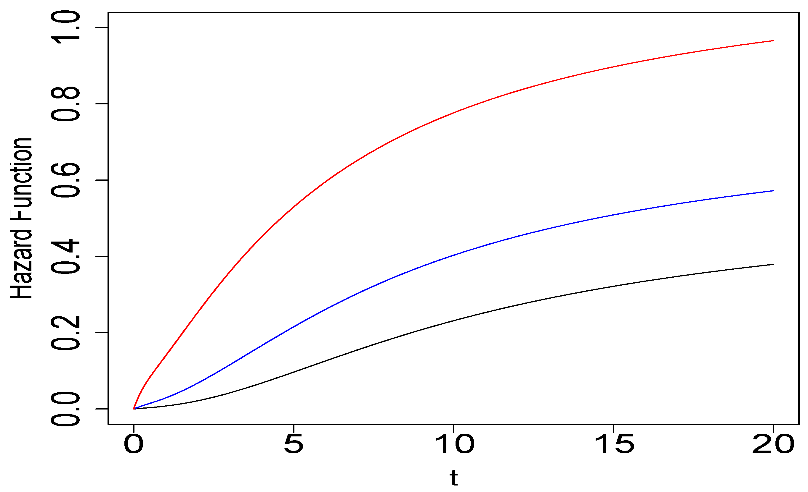
Figure 4.
Plots of the skewness and kurtosis coefficients of the model.
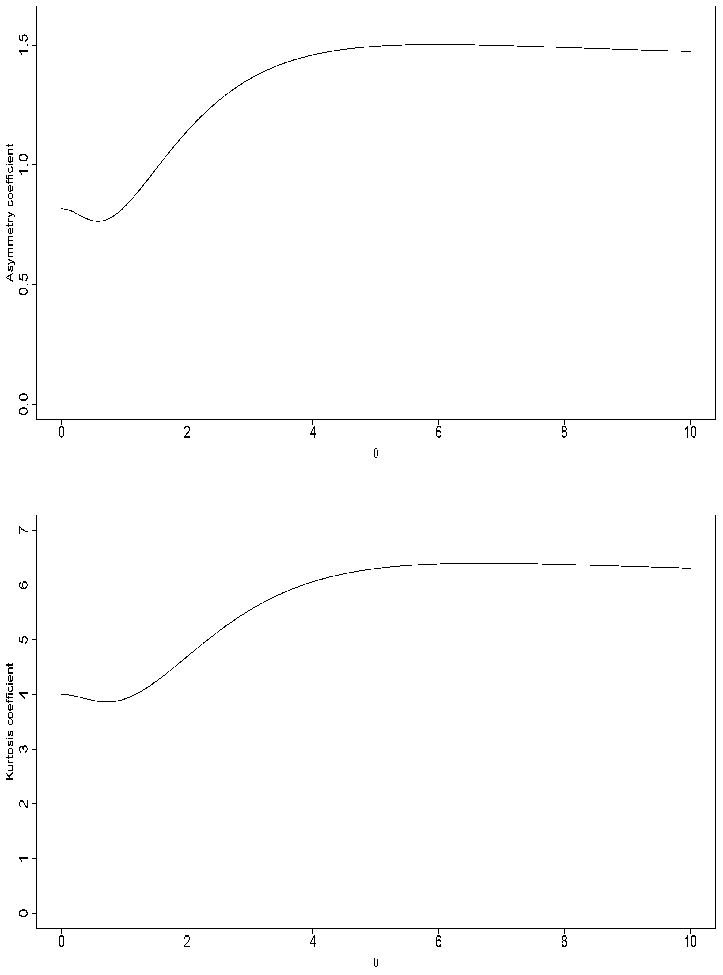
Figure 5.
Q-Q plots of the QRs for AKC distribution
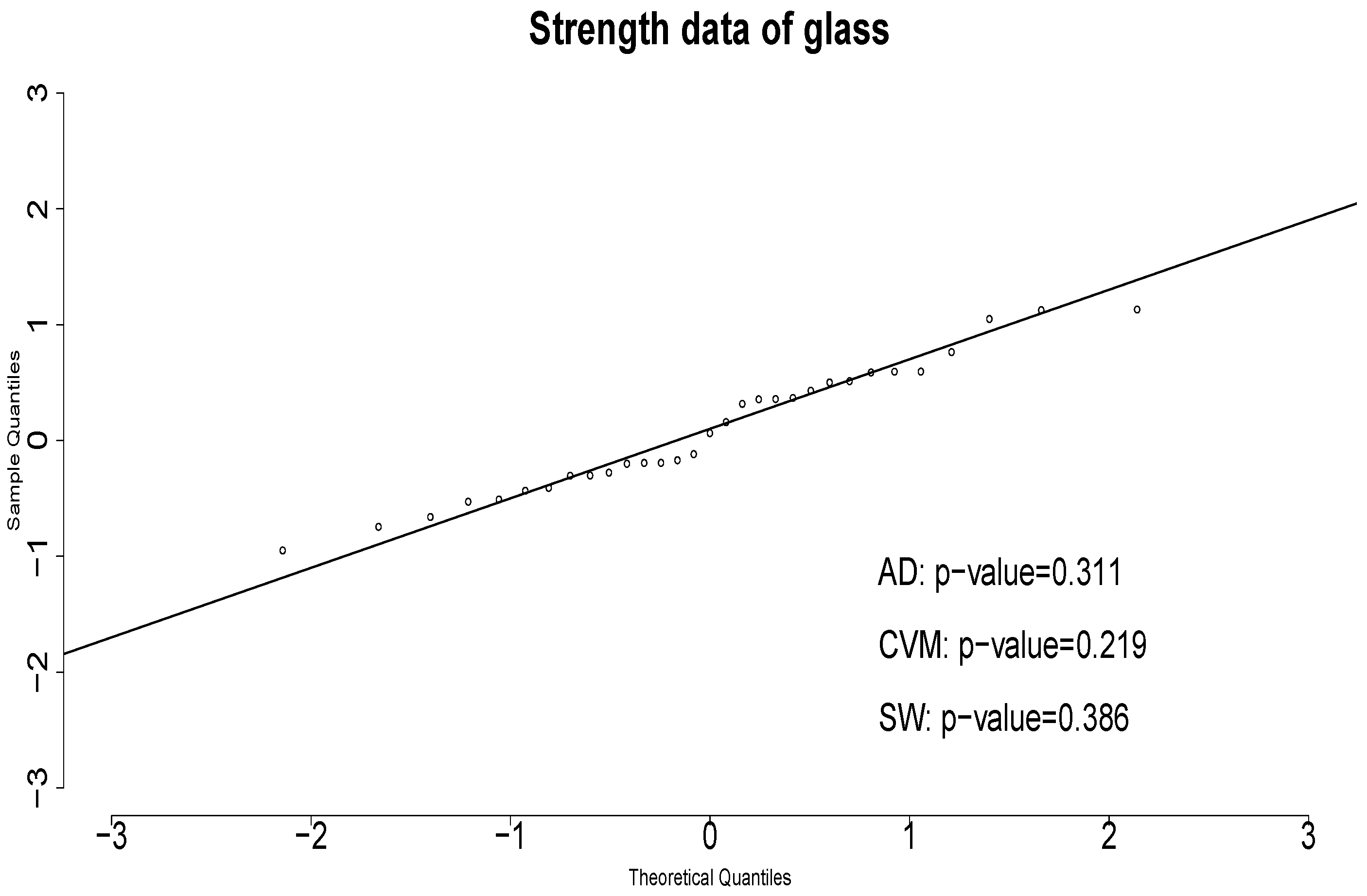
Figure 6.
Q-Q plots of the QRs for AKC distribution
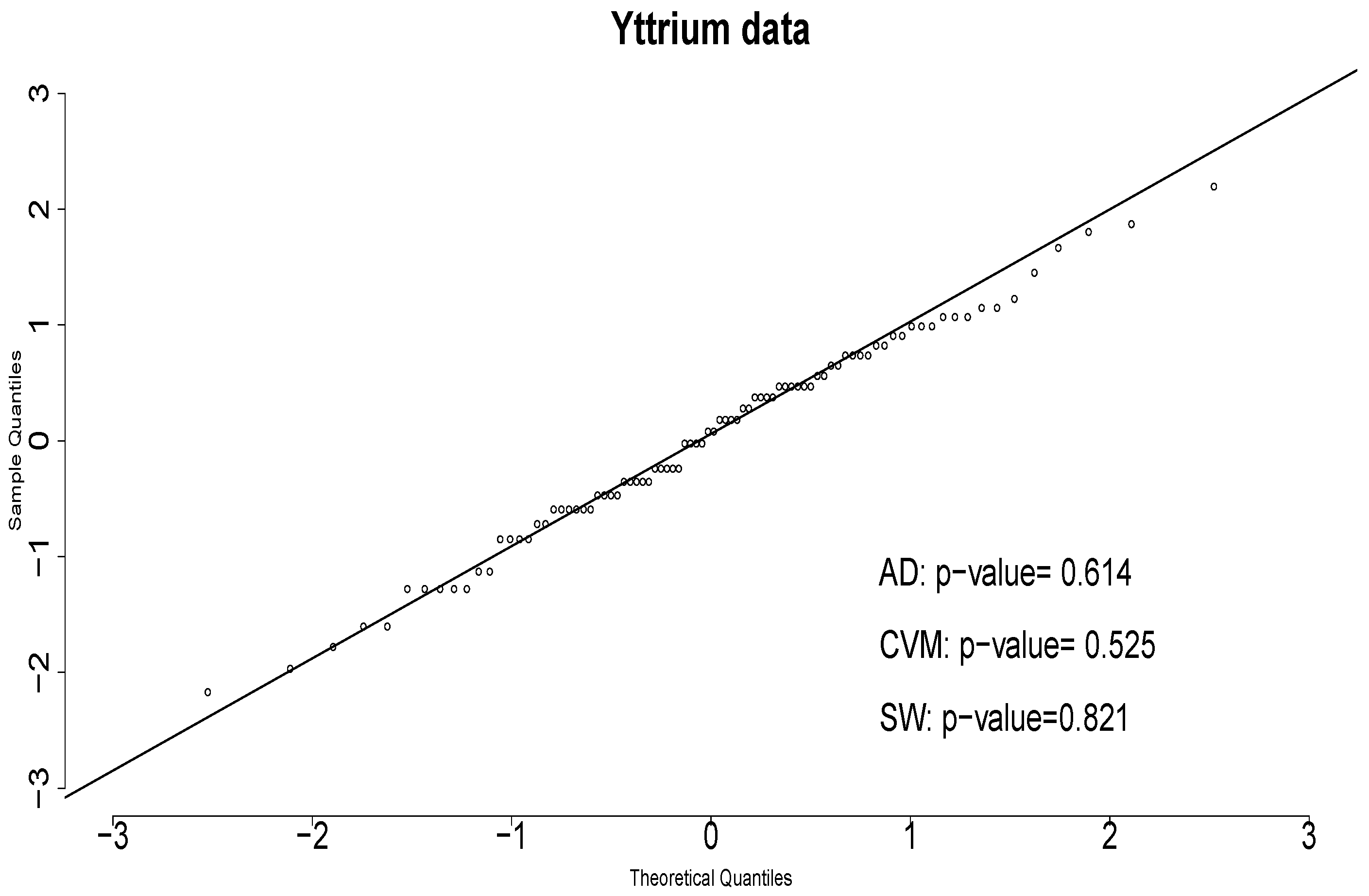

Table 1.
B, SE, RMSE, and CP for the AKC model with .
| n | B | SE | RMSE | CP | |
|---|---|---|---|---|---|
| 0.2 | 20 | 0.001 | 0.018 | 0.018 | 0.942 |
| 50 | 0.001 | 0.012 | 0.012 | 0.949 | |
| 100 | 0.0002 | 0.008 | 0.008 | 0.955 | |
| 0.5 | 20 | 0.002 | 0.046 | 0.046 | 0.952 |
| 50 | 0.001 | 0.029 | 0.029 | 0.952 | |
| 100 | 0.001 | 0.019 | 0.019 | 0.946 | |
| 0.8 | 20 | 0.004 | 0.073 | 0.073 | 0.945 |
| 50 | 0.002 | 0.045 | 0.045 | 0.957 | |
| 100 | 0.002 | 0.031 | 0.031 | 0.953 | |
| 1 | 20 | 0.007 | 0.091 | 0.091 | 0.955 |
| 50 | -0.001 | 0.056 | 0.056 | 0.954 | |
| 100 | 0.004 | 0.040 | 0.040 | 0.941 | |
| 2 | 20 | 0.013 | 0.204 | 0.204 | 0.954 |
| 50 | 0.007 | 0.126 | 0.126 | 0.943 | |
| 100 | 0.008 | 0.088 | 0.088 | 0.948 | |
| 3 | 20 | 0.051 | 0.366 | 0.369 | 0.943 |
| 50 | 0.021 | 0.223 | 0.224 | 0.952 | |
| 100 | 0.009 | 0.155 | 0.155 | 0.950 | |
| 4 | 20 | 0.067 | 0.537 | 0.540 | 0.946 |
| 50 | 0.025 | 0.323 | 0.324 | 0.953 | |
| 100 | 0.028 | 0.238 | 0.240 | 0.949 | |
| 5 | 20 | 0.052 | 0.688 | 0.690 | 0.955 |
| 50 | 0.049 | 0.441 | 0.444 | 0.954 | |
| 100 | 0.016 | 0.309 | 0.309 | 0.948 |
Table 2.
Strength of glass of aircraft window reported by Fuller et al. (1994).
| 18.83 | 20.80 | 21.657 | 23.03 | 23.23 | 24.05 | 24.321 | 25.50 | 25.52 | 25.80 |
| 26.69 | 26.77 | 26.78 | 27.05 | 27.67 | 29.90 | 31.11 | 33.20 | 33.73 | 33.76 |
| 33.89 | 34.76 | 35.75 | 35.91 | 36.98 | 37.08 | 37.09 | 39.58 | 44.045 | 45.29 |
| 45.381 |
Table 3.
Descriptive statistics for strength of glass data.
| n | Median | Mean | Variance | CS | CK |
|---|---|---|---|---|---|
| 31 | 29.90 | 30.81 | 52.61 | 0.405 | 2.287 |
Table 4.
ML Estimates of the , and L Models for Glass Strength Data.
| Model | ML estimate | AIC | BIC |
|---|---|---|---|
| AKC() | 225.868 | 227.302 | |
| AK() | 242.682 | 244.116 | |
| L() | 255.988 | 257.422 |
Table 5.
Yttrium data collected by the Mines Department, University of Atacama, Chile.
| 27 | 20 | 17 | 12 | 33 | 19 | 27 | 27 | 25 | 26 |
| 17 | 13 | 15 | 22 | 24 | 20 | 9 | 20 | 13 | 26 |
| 8 | 27 | 29 | 7 | 33 | 28 | 15 | 36 | 31 | 24 |
| 22 | 12 | 26 | 35 | 15 | 45 | 10 | 27 | 24 | 42 |
| 27 | 23 | 16 | 18 | 28 | 17 | 30 | 18 | 19 | 10 |
| 30 | 30 | 12 | 20 | 17 | 26 | 23 | 35 | 33 | 18 |
| 12 | 22 | 30 | 15 | 19 | 32 | 19 | 19 | 50 | 24 |
| 17 | 34 | 29 | 34 | 32 | 12 | 44 | 39 | 34 | 16 |
| 31 | 22 | 20 | 17 | 18 | 25 |
Table 6.
Descriptive statistics for Yttrium data.
| n | Median | Mean | Variance | CS | CK |
|---|---|---|---|---|---|
| 86 | 23.00 | 23.53 | 79.264 | 0.489 | 3.033 |
Table 7.
ML Estimates of , , and L Models for Yttrium data.
| Model | ML estimate | AIC | BIC |
|---|---|---|---|
| AKC() | 617.956 | 620.411 | |
| AK() | 640.645 | 643.100 | |
| L() | 669.327 | 671.781 |
Disclaimer/Publisher’s Note: The statements, opinions and data contained in all publications are solely those of the individual author(s) and contributor(s) and not of MDPI and/or the editor(s). MDPI and/or the editor(s) disclaim responsibility for any injury to people or property resulting from any ideas, methods, instructions or products referred to in the content. |
© 2024 by the authors. Licensee MDPI, Basel, Switzerland. This article is an open access article distributed under the terms and conditions of the Creative Commons Attribution (CC BY) license (http://creativecommons.org/licenses/by/4.0/).
Copyright: This open access article is published under a Creative Commons CC BY 4.0 license, which permit the free download, distribution, and reuse, provided that the author and preprint are cited in any reuse.


