
Submitted:
17 October 2023
Posted:
19 October 2023
You are already at the latest version
Abstract
In this article we introduce an extension of the Akash distribution. We use the slash 1
methodology to make the kurtosis of the Akash distribution more flexible. We study the general 2
density of this new distribution, some properties, moments, coefficients of asymmetry and kurtosis. 3
Statistical inference is performed using the methods of moments and maximum likelihood via the 4
EM algorithm. A simulation study is carried out to observe the behavior of the maximum likelihood 5
estimator. An application to a real data set with high kurtosis is considered, where it is shown that 6
the new distribution fits better than other extensions of the Akash distribution.
Keywords:
Akash distribution
; Kurtosis
; Maximum likelihood estimation
; Slash distribution
1. Introduction
The slash distribution is an extension of the normal distribution. Its representation is the quotient between two independent random variables, one normal and the other a power of the uniform distribution. In this way we say that S has a slash distribution if:
where , is independent of and , its representation can be seen in Johnson et al. [1]. This distribution has heavier tails than the normal distribution, that is, it has greater kurtosis. Properties of this family are discussed in Rogers and Tukey [2] and Mosteller and Tukey [3]. The maximum likelihood estimation of the location and scale parameters are discussed in Kafadar [4]. Wang and Genton [5] provide a multivariate version of the slash distribution and a multivariate skew version. Gomez et al. [6] and Gómez and Venegas [7] extend the slash distribution using the family of univariate and multivariate elliptic distributions. This methodology to increase the weight of the queues has also been used in distributions with positive support, for example, Gómez et al. [8] in the Birnbaum-Saunders distribution, Olmos et al. [9,10] in the half-normal and generalized half-normal distributions, Astorga et al. [11] in the Muth power distribution and Rivera et al. [12] in the Rayleigh distribution, among others.
Based on the work of Rivera et al. [12], the scale mixture of Rayleigh (SMR) distribution is introduced. We say that with and . Then the probability density function (pdf) of Y is
Also, a necessary distribution in the development of this paper is the gamma distribution, whose pdf is given by
where . Its corresponding cumulative distribution function (cdf) is denoted by:
Shanker [13] introduced the Akash distribution and applied it to real lifetime data sets from medical science and engineering. Thus, we say that a random variable Y has an Akash distribution (AK) with shape parameter if its pdf is given by
where and we denote it by The parameter is a shape parameter, and if we add a scale parameter the pdf is given by
where is a scale parameter, is a shape parameter and we denote it by
Extensions of the AK distribution are carried out by Shanker and Shukla [14,15], among others. Both extensions consider adding a parameter and we will compare them with the new distribution. The two-parameter Akash distribution (TPAD) introduced by Shanker and Shukla [14] has the following pdf:
where and we denote it by
The power Akash distribution (PAD), introduced by Shanker and Shukla [15], has the following pdf:
where and we denote it by
The main objective of this paper is to introduce an extension of the AK distribution given in (6), making use of the slash methodology, in order to obtain a new distribution with greater kurtosis to be able to accomcodate outliers.
The paper evolves as follows: In Section 2 we deliver the new distribution and present its properties. In Section 3 we perform inference using the method of moments and maximum likelihood via the EM algorithm, a simulation study is also carried out. In Section 4 we apply the distribution to a real data set and compare it with other extensions of the AK distribution. In Section 5 we provide some conclusions.
2. New density and its properties
In this section we introduce the representation, density and properties of the new distribution.
2.1. Representation
The representation of this new distribution is given by
where , , Y and Z are independent random variables with . We name the distribution of X slash AK (SAK) and denote it by .
2.2. Density function
The following Proposition shows the pdf of the SAK distribution is generated using the representation given in (9).
Proposition 1.
Let . Then, the pdf of X is given by
where and G is the cdf of the gamma distribution given in .
Proof.
Using the representation given in (9) and procedures based on the Jacobian method, we get the result. □
2.3. Properties
The following Proposition gives the cdf in closed form. It depends on G, which is the cdf of the gamma distribution given in .
Proposition 2.
Let . Then, the cdf of X is given by
where and G is given in .
Proof.
The result follows from a direct application of the definition of a cdf. □
2.3.1. Reliability analysis
The reliability function and the hazard function of the SAK distribution are given in the following corollary.
Corollary 1.
Let . Then, the and of T are given by
- 1.
- 2.
where .
In Figure 2, we introduce the Hazard function of the SAK distribution for several values of and q.
2.3.2. Right tail of the SAK distribution
According to Rolski et al. [16] a distribution has a heavy right tail if
The following result shows that the SAK distribution is heavy-tailed.
Proposition 3.
The distribution of the random variable is heavy-tailed.
Proof.
Applying L’Hospital’s rule twice we have,
□
The following Proposition shows that the SAK distribution can be represented as a scale mixture between the AK and Beta distributions.
Proposition 4.
If and then .
Proof.
The marginal pdf of X is given by
and using , and , this result is obtained. □
The following result shows that when the parameter q tends to infinity, the AK distribution is obtained.
Proposition 5.
Let . If then X converges in law to a random variable .
Proof.
Using its representation we analyze the convergence of this quotient, where and Beta. In the Beta() distribution we have, and . Then, applying Chebychev’s inequality for Z, we have
If then the right hand side of (12) tends to zero, i.e. converges in probability to 0. Also , then we have,
Since , applying Slutsky’s Lemma to , we have
Thus, for increasing values of q, X converges in law to a distribution. □
2.3.3. Moments
In this subsection we obtain the moments of the SAK distribution. To achieve this aim, the next lemma will be useful.
Lemma 1.
Let with . For , exists if and only if and in this case
Proof.
The r-th moment of the random variable is given by Shanker [13], which is , then calculating the r-th moment of the random variable , where is a parameter of scale, the result is obtained. □
The moments of a SAK distribution are given in the following Proposition 6,
Proposition 6.
Let with σ and . For , exists if and only if and in this case
Proof.
Using the representation given in the Proposition 4 and by Lemma 1, we get
Solving the integral gives the result. □
From Proposition 6, the explicit expression of the noncentral moments, , for and the variance of , follow.
Corollary 2.
Let with θ and . From (14), the following noncentral moments and the variance of X, , are obtained
where
Remark 1.
Note that when , , which is the variance of an distribution.
The next Corollary gives the asymmetry coefficient, , of a model.
Corollary 3.
Let with and . Then the skewness coefficient of X is:
Proof.
Recall that
where , and were given in Corollary 2. □
Also, the kurtosis coefficient, , of a distribution is given in the following Corollary.
Corollary 4.
Let with and . Then the kurtosis coefficient of X is
where , , and
Proof.
Recall that
where , , , and were given in Corollary 2. □
Remark 2.
It can be verified that for skewness and kurtosis coefficients converge to and respectively, which coincide with the corresponding coefficients for the AK(θ) distribution (see Shanker, 2015).
The results of Table 2 show that the values of the skewness and kurtosis coefficients depend on the parameters and q and that as q decreases, the skewness and kurtosis coefficients increase. On the other hand, as q increases, the skewness and kurtosis coefficients are those of the AK() distribution (Proposition 5).
3. Inference
In this section we study the estimation the parameters by the method of moments and ML via the EM algorithm. We also carry out some simulations to study the behavior of the ML estimators.
3.1. Method of moment estimators
Let be a random sample from . Consider the first two sample moments, denoted by and , respectively.
Proposition 7.
Given a random sample from with , the moment method estimators of θ and q are
where (16) must be solved numerically to obtain . Then must be replaced in (15) to get .
3.2. ML estimation
Let be a random sample from . Then the log-likelihood function is
where Taking partial derivatives in with respect to and q and setting them equal to zero, we get
where , and Solving numerically this system of equations to find the ML estimates may be a difficult task due to the functions it involves. However, an EM algorithm can be implemented (see Dempster et al. [17]) to obtain the ML estimates. The following subsection is dedicated to achieving this goal.
3.3. EM Algorithm
An alternative stochastic representation for the SAK model is given by
where and , represent non-observable variables. This representation can be used for an alternative estimation procedure based on the EM algorithm (Dempster et al. [17]). In this context, the observed data are given by , where . The vectors and are the latent variables and the vector are the complete data. Note that the joint distribution of is given by
Therefore, up to a constant that does not depend on the vector of parameters , the complete log-likelihood function for the model is given by
With this, the expected value of , given the observed data, is
where and . Note that
where , is the cdf for the gamma model and denotes de gamma distribution with shape a and rate b truncated in the interval (0,1). Therefore, using properties of conditional expectations, we have and by (19) such expectations are simple to be computed. In a similar manner, we can compute , obtaining as results
Therefore, the kth iteration of the algorithm comprises the following steps:
- E-step: Given and , for compute and using equations (20) and (21), respectively.
- M1-step: Update as
- M2-step: Update as the solution for the non-linear equation
The E, M1 and M2 steps are repeated until convergence is obtained, i.e. until the maximum distance between the estimate obtained in two consecutive iterations is less than a specified value.
In the following subsection we run some simulations to study the behavior of the ML estimators.
3.4. Simulation study
Table 3 shows the empirical bias (bias), the average of the standard errors (SE), the root of the empirical mean squared error (RMSE), and the 95% coverage probability (CP) based on the asymptotic distribution for the ML estimators of the parameters. Table 3 shows that the performance of the estimator improves as n increases.
4. Application
In this section we analyze a real data set showing that the SAK distribution can be more appropriate than other commongly used distributions to model heavy right-tailed data. The data correspond to plasma beta-carotene levels (ng/ml) of 314 patients. This data set contains 14 variables and is available online at “http://Lib.stat.cmu.edu/datasets/Plasma Retinol”. In this study, we consider the variable Betaplasma. The medical interest in this variable comes from the fact that low levels of plasma beta-carotene may be associated with higher risk of developing certain types of cancer. In Table 4 we present some descriptive statistics including the sample skewness, , and sample and kurtosis . We may observe high kurtosis in this data set.
The moment estimates for the parameters of the SAK distribution are and . These estimates are useful starting values, required to implement maximum likelihood estimation using numerical methods. Table 5 shows the ML estimates for the parameters of the PAD, SMR and SAK models. For each model we report the value of the log-likelihood. It can be seen that the SAK model presented a larger value of log-likelihood than the other models.
In order to compare the fit of the distributions, we considered the usual Akaike information criterion (AIC), introduced by Akaike [18], and the Bayesian information criterion (BIC), proposed by Schwarz [19]. It is known that AIC= and BIC= where k is the number of parameters in the model, n is the sample size and is the maximized value of the log-likelihood function. Table 6 shows the AIC and BIC for each model, indicating that the SAK distribution leads to a better fit than the other distributions. Figure 3 presents the histogram for the data together with the fitted densities.
We also calculated the quantile residuals (QR). If the model is appropriate for the data, the QR should be a sample of the standard normal distribution (see Dunn and Smyth, [20]). This assumption can be validated with traditional normality tests, such as the Anderson-Darling (AD), Cramér-von Mises (CVM) and Shapiro-Wilkes (SW) tests. Figure 4 shows the qqplot of the quantile residuals of the three fitted distributions. All three tests suggest that the SAK model provides a better fit for this data set.
5. Discussion
This paper presents an extension of the AK distribution based on the slash methodology. Some properties of this new distribution are derived. It is also compared with two other distributions using a real data set. Estimation is done through ML via the EM algorithm. The new SAK distribution is an alternative to fit heavy-tailed right-skewed data. Additional features of the SAK distribution are:
- The distribution has two representations, one based on the quotient of two independent random variables and another based on a scale mixture between the AK and Beta distributions.
- The pdf, cdf and hazard function of the SAK distribution are explicit and are represented by the cdf of the gamma distribution.
- The distribution has a heavy right tail.
- The distribution contains the AK distribution as a limit, that is, when the parameter q tends to infinity in the distribution SAK, the AK distribution is obtained.
- The moments and the coefficients of skewness and kurtosis are explicit.
- In the application, observing the AIC and BIC and the Anderson-Darling, Cramér-von Mises and Shapiro-Wilkes statistical tests, we may conclude that the SAK distribution fits the Betaplasma data set better than the PAD and SMR distributions, which are also extensions of the AK distribution.
References
- Jonhson, N.L., Kotz, S., and Balakrishnan, N.1995.Continuous univariate distributions. Vol 1, 2nd edn. New York: Wiley.
- Rogers, W.H., Tukey, J.W. 1972. Understanding some long-tailed symmetrical distributions. Statist. Neerlandica 26 :211-226. [CrossRef]
- Mosteller, F., Tukey, J.W. 1977. Data analysis and regression. Addison-Wesley, Reading, MA.
- Kafadar, K. 1982. A biweight approach to the one-sample problem. J. Amer. Statist. Assoc. 77 :416-424. [CrossRef]
- Wang, J., Genton, M.G. 2006. The multivariate skew-slash distribution. Journal Statistical Planning and Inference 136 :209-220. [CrossRef]
- Gómez, H.W., Quintana, F.A., Torres, F. J. 2007. A New Family of Slash-Distributions with Elliptical Contours. Statistics and Probability Letters 77(7):717-725. [CrossRef]
- Gómez, H.W., Venegas, O. 2008. Erratum to: A new family of slash-distributions with elliptical contours [Statist. Probab. Lett. 77 (2007) 717-725]. Statistics and Probability Letters 78 (14):2273-2274. [CrossRef]
- Gómez, H.W., Olivares-Pacheco, J.F., Bolfarine, H. 2009. An extension of the generalized birnbaun-saunders distribution. Statistics and Probability Letters 79 (3):331-338. [CrossRef]
- Olmos, N.M., Varela, H., Gómez, H.W. and Bolfarine, H. 2012. An extension of the half-normal distribution. Statistical Papers 53 :875-886. [CrossRef]
- Olmos, N.M., Varela, H., Bolfarine, H., Gómez, H.W. 2014. An extension of the generalized half-normal distribution. Statistical Papers 55:967-981. [CrossRef]
- Astorga, J.M., Reyes, J., Santoro, K.I., Venegas, O., Gómez, H.W. 2020. A Reliability Model Based on the Incomplete Generalized Integro-Exponential Function. Mathematics 8:1537. [CrossRef]
- Rivera P.A., Barranco-Chamorro I., Gallardo D.I., Gómez H.W. 2020. Scale Mixture of Rayleigh Distribution. Mathematics 8(10):1842. [CrossRef]
- Shanker, R. 2015. Akash Distribution and Its Applications. International Journal of Probability and Statistics 4(3):65-75. [CrossRef]
- Shanker, R., Shukla, K.K. 2017a. On Two-Parameter Akash Distribution. Biometrics & Biostatistics International Journal 6(5):00178. [CrossRef]
- Shanker, R., Shukla, K.K. 2017b. Power Akash Distribution and Its Application. Journal of Applied Quantitative Methods 12(3):1-10.
- Rolski, T., H. Schmidli, V. Schmidt, and J. Teugel. 1999. Stochastic Processes for Insurance and Finance. John Wiley & Sons.
- Dempster. A.P.; Laird. N.M.; Rubim. D.B. 1977. Maximum likelihood from incomplete data via the EM algorithm (with discussion). J. R. Stat. Soc. Ser. B, 39, 1–38.
- Akaike, H. 1974. A new look at the statistical model identification. IEEE Transactions on Automatic Control, 19(6), 716-723. [CrossRef]
- Schwarz, G. 1978. Estimating the dimension of a model. Ann. Statist., 6(2), 461-464. [CrossRef]
- Dunn, P.K., Smyth, G.K. 1996. Randomized Quantile Residuals. Journal of Computational and Graphical Statistics, 5(3), 236-244. [CrossRef]
Figure 1.
Left side: Examples of the SAK() (in black), SAK() (in blue), SAK() (in red). Right side: Examples of the SAK() (in black), SAK() (in blue), SAK() (in red).
Figure 1.
Left side: Examples of the SAK() (in black), SAK() (in blue), SAK() (in red). Right side: Examples of the SAK() (in black), SAK() (in blue), SAK() (in red).
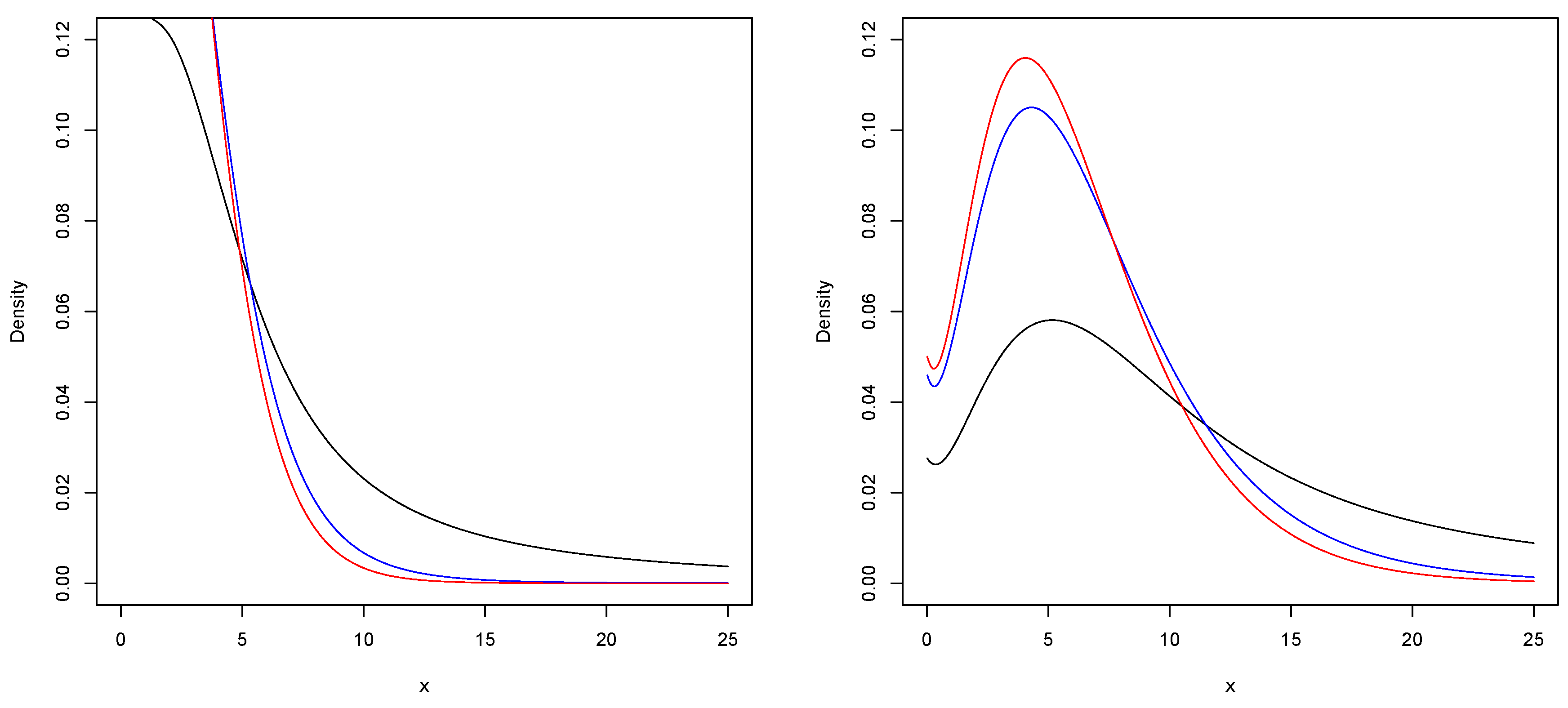
Figure 2.
Hazard function of the SAK() distribution (in black), SAK() distribution (in blue), SAK() distribution (in red).
Figure 2.
Hazard function of the SAK() distribution (in black), SAK() distribution (in blue), SAK() distribution (in red).
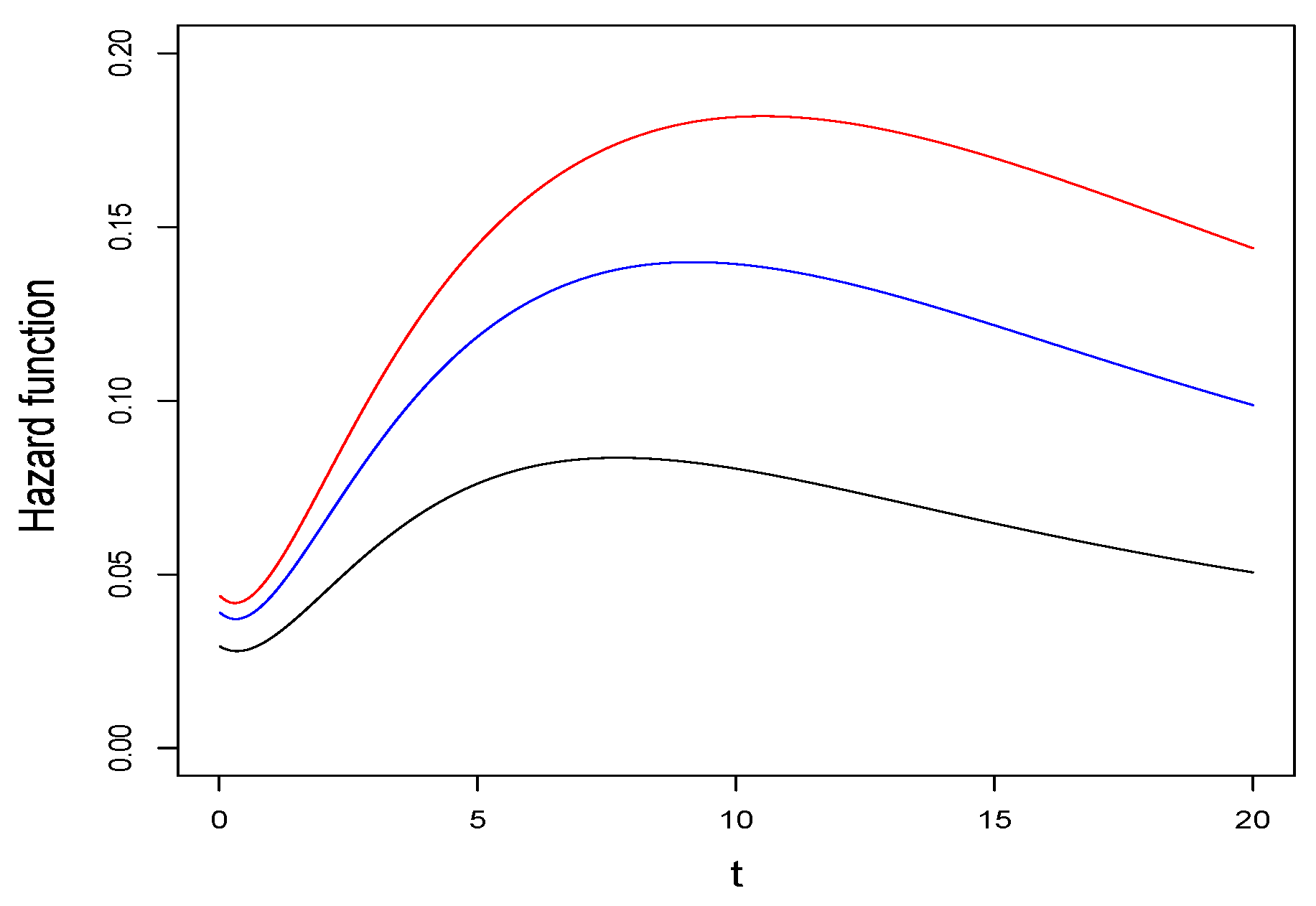
Figure 3.
Betaplasma: Histogram and fitted PAD pdf (in red), SMR pdf (in blue) and SAK pdf (in black).
Figure 3.
Betaplasma: Histogram and fitted PAD pdf (in red), SMR pdf (in blue) and SAK pdf (in black).
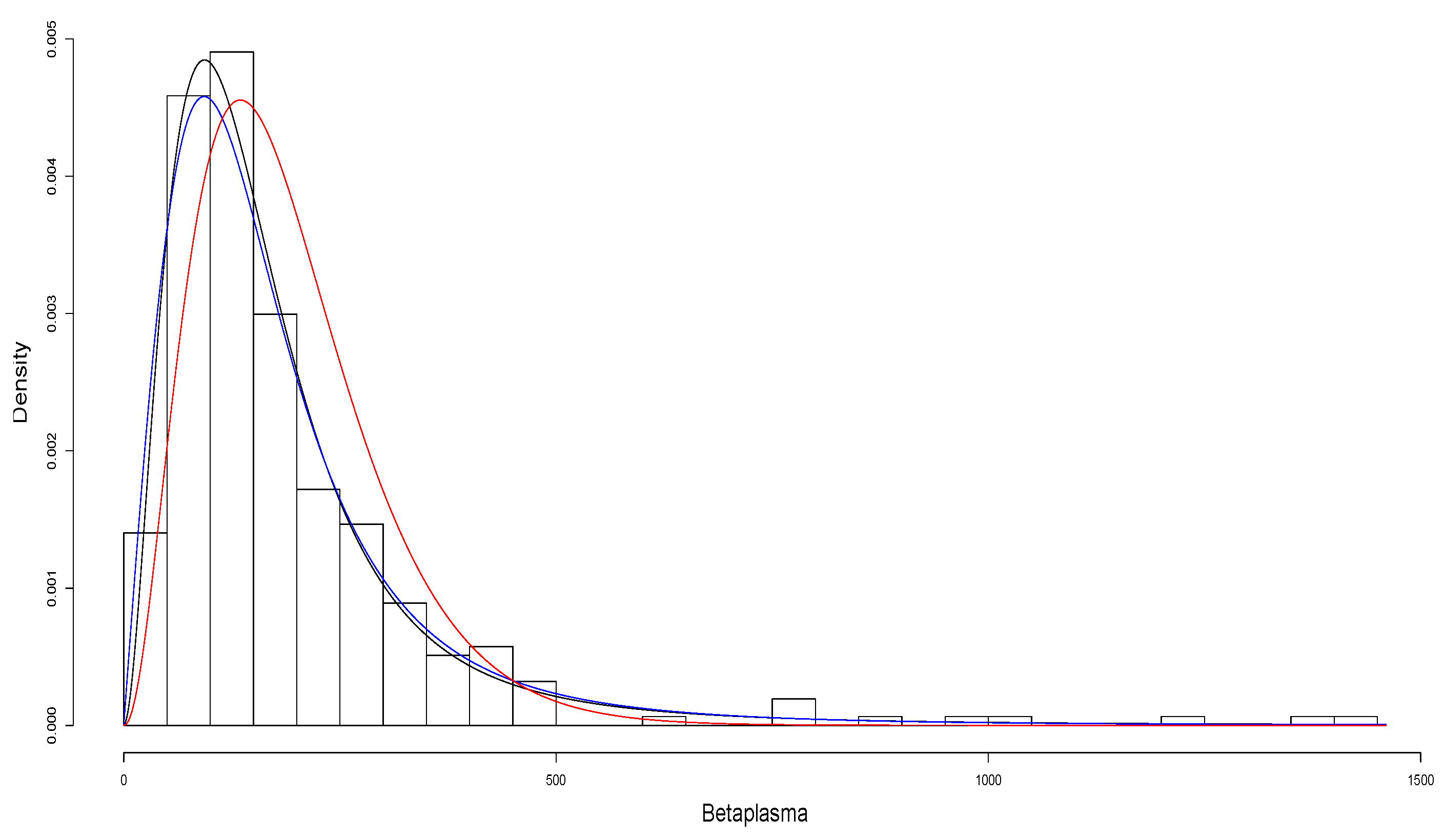
Figure 4.
qqplots of the quantile residuals for the fitted models, together with the p-values of the AD, CVM and SW normality tests.
Figure 4.
qqplots of the quantile residuals for the fitted models, together with the p-values of the AD, CVM and SW normality tests.
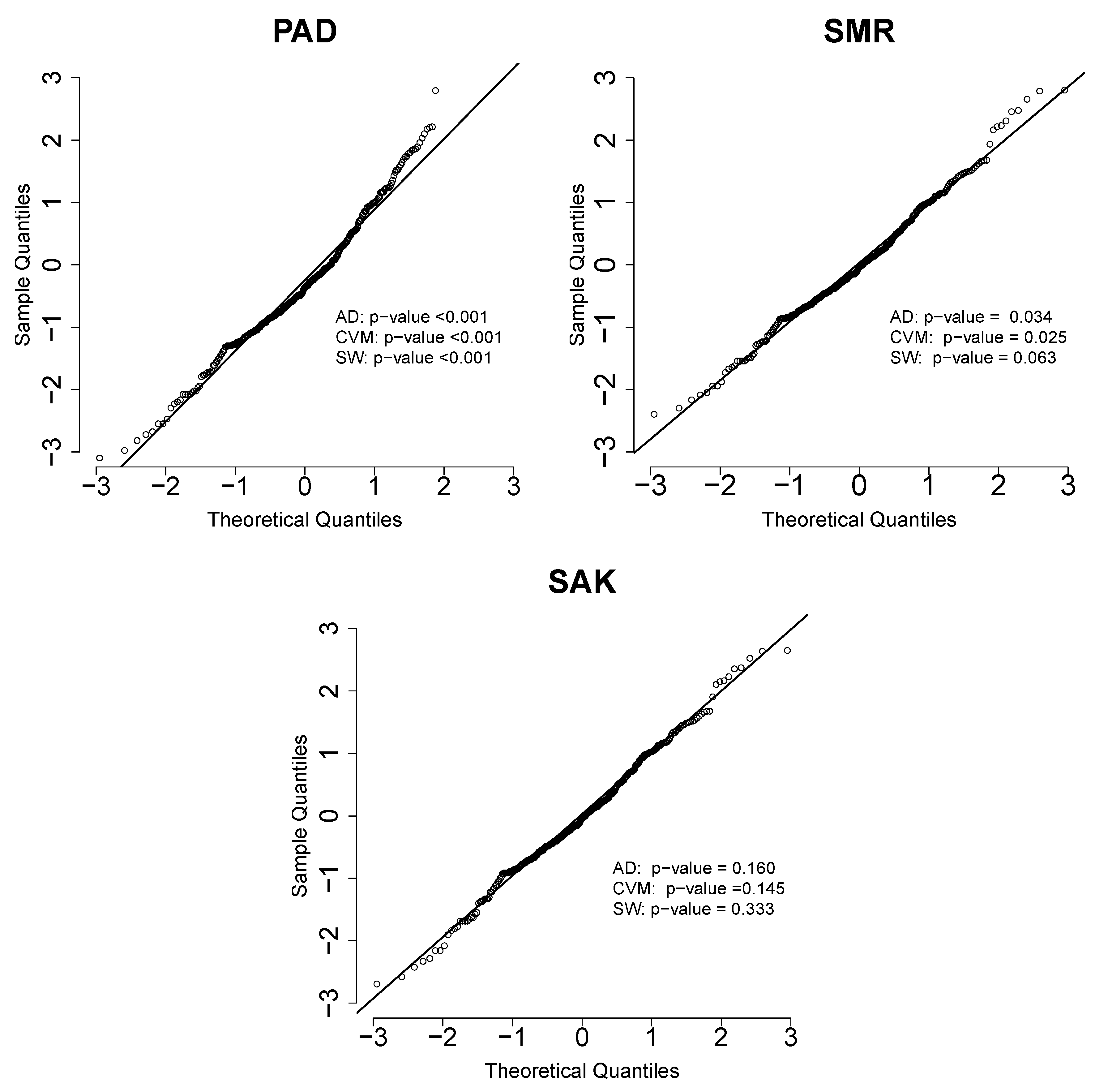

Table 1.
Tail comparisons of the AK and SAK distributions.
| Distribution | Distribution | ||||
| SAK(1,1) | SAK(0.5,1) | ||||
| SAK(1,5) | SAK(0.5,5) | ||||
| SAK(1,10) | SAK(0.5,10) | ||||
| AK(1) | AK(0.5) |
Table 2.
Skewness and kurtosis of the SAK distribution for various values of the shape parameters.
| q | |||
| 5 | |||
| 1 | |||
| 6 | |||
| 1 | |||
| 7 | |||
| 1 | |||
| 10 | |||
| 1 | |||
| 100 | |||
| 1 | |||
| ∞ | |||
| 1 |
Table 3.
Estimated bias, SE, RMSE and CP of the ML estimators of the parameters of the SAK model for different values of n
Table 3.
Estimated bias, SE, RMSE and CP of the ML estimators of the parameters of the SAK model for different values of n
| n = 30 | n = 50 | n = 100 | n = 200 | n = 500 | ||||||||||||||||||
| q | estimator | bias | SE | RMSE | CP | bias | SE | RMSE | CP | bias | SE | RMSE | CP | bias | SE | RMSE | CP | bias | SE | RMSE | CP | |
| 0.5 | 0.5 | -0.002 | 0.119 | 0.124 | 0.914 | -0.004 | 0.092 | 0.094 | 0.930 | -0.001 | 0.065 | 0.066 | 0.937 | 0.000 | 0.046 | 0.046 | 0.946 | 0.000 | 0.029 | 0.029 | 0.947 | |
| 0.036 | 0.122 | 0.139 | 0.961 | 0.025 | 0.092 | 0.100 | 0.958 | 0.012 | 0.063 | 0.065 | 0.952 | 0.005 | 0.043 | 0.044 | 0.952 | 0.001 | 0.027 | 0.027 | 0.951 | |||
| 1.0 | -0.004 | 0.110 | 0.114 | 0.918 | -0.003 | 0.085 | 0.086 | 0.931 | -0.002 | 0.060 | 0.061 | 0.940 | -0.001 | 0.043 | 0.043 | 0.946 | 0.000 | 0.027 | 0.027 | 0.946 | ||
| -0.159 | 0.236 | 0.253 | 0.924 | -0.112 | 0.161 | 0.171 | 0.929 | -0.087 | 0.108 | 0.115 | 0.939 | -0.059 | 0.074 | 0.081 | 0.948 | -0.046 | 0.046 | 0.051 | 0.948 | |||
| 2.0 | -0.003 | 0.105 | 0.107 | 0.931 | -0.003 | 0.081 | 0.082 | 0.939 | -0.002 | 0.057 | 0.058 | 0.940 | -0.001 | 0.040 | 0.041 | 0.945 | 0.000 | 0.025 | 0.026 | 0.947 | ||
| -0.137 | 0.597 | 0.622 | 0.904 | -0.125 | 0.395 | 0.420 | 0.924 | -0.077 | 0.233 | 0.250 | 0.932 | -0.041 | 0.151 | 0.162 | 0.942 | -0.023 | 0.092 | 0.095 | 0.948 | |||
| 3.0 | 0.5 | 0.136 | 1.063 | 1.236 | 0.891 | 0.095 | 0.794 | 0.861 | 0.915 | 0.035 | 0.537 | 0.556 | 0.927 | 0.013 | 0.373 | 0.380 | 0.940 | 0.005 | 0.234 | 0.235 | 0.947 | |
| 0.059 | 0.156 | 0.206 | 0.963 | 0.030 | 0.110 | 0.124 | 0.958 | 0.015 | 0.075 | 0.079 | 0.955 | 0.009 | 0.052 | 0.054 | 0.953 | 0.003 | 0.032 | 0.033 | 0.952 | |||
| 1.0 | 0.104 | 0.982 | 1.112 | 0.896 | 0.060 | 0.729 | 0.786 | 0.912 | 0.028 | 0.499 | 0.517 | 0.929 | 0.012 | 0.347 | 0.354 | 0.941 | 0.003 | 0.218 | 0.219 | 0.948 | ||
| -0.087 | 0.398 | 0.446 | 0.892 | -0.057 | 0.245 | 0.296 | 0.925 | -0.021 | 0.145 | 0.188 | 0.938 | -0.012 | 0.097 | 0.117 | 0.948 | -0.002 | 0.060 | 0.066 | 0.947 | |||
| 2.0 | 0.145 | 0.976 | 1.070 | 0.922 | 0.068 | 0.709 | 0.747 | 0.929 | 0.018 | 0.478 | 0.491 | 0.934 | 0.006 | 0.332 | 0.339 | 0.941 | 0.000 | 0.208 | 0.210 | 0.946 | ||
| -0.105 | 1.025 | 1.090 | 0.915 | -0.084 | 0.724 | 0.790 | 0.924 | -0.069 | 0.440 | 0.485 | 0.935 | -0.048 | 0.255 | 0.282 | 0.942 | -0.008 | 0.140 | 0.155 | 0.948 | |||
| 10.0 | 0.5 | 0.595 | 4.688 | 5.331 | 0.882 | 0.291 | 3.484 | 3.709 | 0.901 | 0.126 | 2.400 | 2.470 | 0.925 | 0.088 | 1.684 | 1.706 | 0.942 | 0.019 | 1.056 | 1.049 | 0.944 | |
| 0.069 | 0.175 | 0.184 | 0.964 | 0.035 | 0.113 | 0.128 | 0.963 | 0.016 | 0.075 | 0.080 | 0.957 | 0.007 | 0.052 | 0.053 | 0.951 | 0.003 | 0.032 | 0.033 | 0.951 | |||
| 1.0 | 0.559 | 4.440 | 4.910 | 0.904 | 0.222 | 3.260 | 3.453 | 0.910 | 0.102 | 2.248 | 2.328 | 0.926 | 0.059 | 1.574 | 1.600 | 0.941 | 0.009 | 0.987 | 0.980 | 0.948 | ||
| -0.097 | 0.508 | 0.631 | 0.899 | -0.051 | 0.284 | 0.389 | 0.903 | -0.031 | 0.152 | 0.199 | 0.939 | -0.023 | 0.098 | 0.117 | 0.948 | -0.012 | 0.060 | 0.080 | 0.948 | |||
| 2.0 | 0.885 | 4.575 | 4.757 | 0.935 | 0.389 | 3.286 | 3.316 | 0.937 | 0.172 | 2.209 | 2.217 | 0.944 | 0.035 | 1.533 | 1.546 | 0.947 | -0.006 | 0.955 | 0.955 | 0.947 | ||
| -0.068 | 1.224 | 1.222 | 0.924 | -0.057 | 0.834 | 0.950 | 0.931 | -0.037 | 0.440 | 0.483 | 0.935 | -0.027 | 0.305 | 0.313 | 0.942 | -0.018 | 0.149 | 0.159 | 0.943 | |||
Table 4.
Descriptive statistics for the data set.
| n | ||||
| 314 | 190.4968 | 33480.72 | 3.536562 | 16.8145 |
Table 5.
ML estimates for PAD, SMR and SAK models.
| Parameter estimates | PAD (SE) | SMR (SE) | SAK (SE) |
| 0.012 (0.003) | 16998.167 (3399.076) | 0.027 (0.002) | |
| 1.052 (0.038) | − | − | |
| q | − | 2.926 (0.385) | 2.331 (0.294) |
| Log-likelihood | −1953.632 | −1910.472 | −1908.147 |
Table 6.
AIC and BIC for fitted models.
| Criterion | PAD | SMR | SAK |
| AIC | 3911.264 | 3824.944 | 3820.294 |
| BIC | 3918.763 | 3832.443 | 3827.793 |
Disclaimer/Publisher’s Note: The statements, opinions and data contained in all publications are solely those of the individual author(s) and contributor(s) and not of MDPI and/or the editor(s). MDPI and/or the editor(s) disclaim responsibility for any injury to people or property resulting from any ideas, methods, instructions or products referred to in the content. |
© 2023 by the authors. Licensee MDPI, Basel, Switzerland. This article is an open access article distributed under the terms and conditions of the Creative Commons Attribution (CC BY) license (http://creativecommons.org/licenses/by/4.0/).
Copyright: This open access article is published under a Creative Commons CC BY 4.0 license, which permit the free download, distribution, and reuse, provided that the author and preprint are cited in any reuse.


