
Submitted:
17 December 2024
Posted:
18 December 2024
You are already at the latest version
Abstract
Due to the geostrophic balance, horizontal divergence-free is often assumed when analyzing large-scale oceanic flows. However, the geostrophic balance is a leading-order approximation. We investigate the statistical feature of weak horizontal compressibility in the Gulf of Mexico by analyzing drifter data (the Grand LAgrangian Deployment (GLAD) experiment and the LAgrangian Submesoscale ExpeRiment (LASER)) based on the asymptotic probability density function of the angle between velocity and acceleration difference vectors in a strain-dominant model. The results reveal a notable divergence at scales between 10 km and 300 km, which is stronger in winter (LASER) than in summer (GLAD). We conjecture that the divergence is induced by wind stress with its curl parallel to the earth’s rotation.
Keywords:
homogeneous turbulence
; isotropic turbulence
; oceanic surface flow
; ocean surface drifter
; skewness of horizontal divergence
1. Introduction
In large-scale oceanic flows, the Coriolis effect and the pressure gradient dominate the horizontal momentum balance [1,2]. When the Coriolis parameter is a constant, geostrophic flow is horizontally non-divergent. This horizontal non-divergent condition simplifies many theoretical analyses. For instance, the third-order structure function theory with the incompressible condition can be used to study the direction of energy cascades in the atmosphere [3] and ocean [4,5].
Geostrophic balance describes the oceanic mesoscale to the leading order of small Rossby number, while at submeso and smaller scales, horizontal divergence can be of leading order [6] and even mesoscale motion can have weak horizontal divergence. Second-order structure functions can be constructed to detect the amplitude of this compressibility [7], but the sign of horizontal velocity divergence is unknown.
We go beyond the velocity structure function and study the combined information from the velocity difference vector and acceleration difference vector . In three-dimensional (3D) turbulence, the ensemble average of their dot product, denoted as , is found to be a constant under a fixed energy cascading rate with its sign corresponding to the direction of cascade in the inertial range, which is justified by experiments [8]. Thus, it is natural to study the angle between and . In a simple model with constant strain rates and without rotation, the probability density function (p.d.f.) of is related to the aspect ratio of the eigenvalues of the velocity strain rate tensor. The p.d.f. of under this model fits well with the p.d.f. from experiments [9].Therefore, it is possible to obtain information about the eigenvalues of the strain rate tensor from the p.d.f. of .
This paper treats the oceanic surface flow as a projection of 3D flow. In this sense, the eigenvalues of the strain rate tensor reveal the compressibility of the surface flow. By analyzing drifter data in the Gulf of Mexico, we aim to detect the amplitude and sign of the horizontal divergence in oceanic surface flow.
The structure of the rest of this paper is as follows. Section 2 introduces the theoretical background and methods for analyzing the drifter data. Then we show the main results in Section 3. Finally, we discuss the phenomenon found from the results and propose the possible physics in Section 4. Details of data processing and error estimation will be shown in Appendix A and Appendix B. More fitting results are displayed in Appendix C.
2. Theories and Methods
We build a model that captures the relation between the angle of acceleration and velocity difference vectors and the divergence at a certain scale, which is inspired by Gibert et al. (2012) [9]. Since drifters may be distributed at strain-dominant regions around vortices in a diffusion process [10], we consider that at each scale, random strains dominantly impact pair separation. Thus we keep the model to be irrotational.
2.1. Random Strain Model
We can start from a simple case where the flow has constant strain rates and does not rotate. Consider a 3D incompressible flow, then the velocity gradient tensor is constant and symmetric with zero trace:
For simplicity, we consider a linear velocity profile and the corresponding acceleration can be expressed as
Here, we chose the Cartesian coordinates O-, where the x-axis points to the East, the y-axis points to the North and the z-axis is vertically upwards. The indices range from 1 to 3, and each pair of repeating indices represents the corresponding summation from 1 to 3. The velocity is also denoted as , where represent the unit vectors of the axes respectively.
We can perform an orthogonal diagonalization since is assumed symmetric. Choosing the principal coordinates O-, we obtain
where are the eigenvalues of . Here, we applied the incompressibility condition
and .
For the large-scale oceanic flow, due to the dominant geostrophic balance, the principal axes and lie close to the x-y plane. Therefore, it is reasonable to assume and the -axis is parallel to the z-axis. Under these assumptions, the horizontal velocity divergence is not zero:
where is the horizontal gradient.
Thus, a divergent flow would correspond to a negative and a negative , and a convergent flow would correspond to a positive and a positive .
Considering two-dimensional (2D) drifter pair dispersion in the ocean, the relative position vector between two drifters can be expressed as
where and are the unit vectors of the axes and , is the distance between the drifters, and represents the angle between and . When is fixed, the velocity and acceleration difference vectors can be expressed as
and
Let be the angle between and . We can obtain the exact expression of :
which is independent of and .
Oceanic flows can be different when the scale changes. To apply the model to real oceanic flows, we assume () and to be functions of the scale, i.e. functions of in a 2D drifter pair dispersion. We further assume that the angle is a random variable (r.v.), to capture the changing direction of the principal axes and drifter pairs. When the flow is assumed isotropic, is independent of . Considering (9), for a fixed scale, the quantity as a function of is also a r.v. Our aim is to obtain from the distribution of under different scales.
2.2. Probability Distribution of
The exact expression of as a function of (9) has a complicated form which is not easily applicable to data analysis. As has been discussed above, the dominant geostrophic balance implies , so we can expand into a series of :
At the first order, we obtain
It is reasonable to reset instead of to be the independent variable. We introduce the following notations for convenience:
The reverse function of (11) exists when , and the 1st-order relations become
To the second order, these relations become
The results of our study will show that is on the order of for oceanic surface flow, making the 1st-order expansion a good approximation.
The probability distribution of can be expressed by the distribution of (or ) in an asymptotic form. Consider a simple case when is uniformly distributed over . The p.d.f. of was derived in the 2D incompressible case with [9]:
To the 1st order of , We derive the expression of p.d.f. of as
This expression introduces an asymmetric part with as the leading order, which inspires us to describe the influence of non-zero by even-odd decomposition.
2.3. Procedure for Analyzing Oceanic Surface Flow
Hinted by (16), we decompose the p.d.f.s into the even and odd parts
The analysis will be based on the following assumptions:
Assumption 1.
Assuming that in the even-odd decomposition , . So we can introduce a bookkeeping parameter ϵ to mark the smallness of the odd part of the p.d.f., i.e.
Assumption 2.
is small in oceanic flows, i.e. . Hence the discussion in Section 2.2 holds valid.
Assumption 3.
, i.e. the odd p.d.f. of is dominated by α instead of ϵ. Thus, α measures the skewness of p.d.f. of the angular distribution of drifter pairs.
The p.d.f. of can be derived through a simple relation: , where always holds non-negative under assumption 2. Denoting with and , we have:
where we omitted the second-order term. Combined with assumption 1 and assumption 3, we get the even-odd decomposition for :
where the skewness of p.d.f. of the angular distribution is captured by .
Considering the decomposition in (20), we can use the even part to express the odd part, thus obtaining the by fitting. Here we use the least square method for fitting.
After obtaining the odd and even parts of the p.d.f. from data, we introduce the loss function as
where
then we obtain by minimizing :
Here the sequence represents the data points, and it is chosen to be a finite arithmetic sequence with a common difference of .
In our model, is closely related to horizontal compressibility by (5). If itself is a r.v. with its p.d.f. denonted as , assuming that is negligible when , then the relation between x and y is 1-to-1, therefore the in (20) can be understood as its expectation . Thus, we may expect to obtain a statistical average of horizontal velocity divergence, i.e. the asymmetry towards divergence or convergence, by the sign of .
3. Results
In this study, we analyze two data sets of drifter motion from the Grand LAgrangian Deployment (GLAD) experiment and the LAgrangian Submesoscale ExpeRiment (LASER). Drifters were deployed in the Gulf of Mexico in Summer/July to August 2012 (GLAD) [11] and in Winter/January to February 2016 (LASER) [12]. The locations of drifters are tracked using the Global Positioning System (GPS) within a nominal position error less than 10 m [5]. We think these two sets of data can reflect the velocity of oceanic surface flows precisely at the scales studied here.
The p.d.f. of to the zeroth order is (15) when is uniformly distributed over . Therefore, we can do a rough comparison between the actual p.d.f. of and (15). Choose the data in LASER and around 33 km as an example, and the result is shown in Figure 1. Details of data processing are written in Appendix A. We find that (15) can already qualitatively describe the p.d.f. of , i.e. distributing around has the maximum probability, while the p.d.f. changes little and lies below around . The dimensionless quantity , which may represent the compressibility by (5), appears in the first-order expansion. Then, a rough estimation of can be done according to (16).
Section 2.3 provides a method to obtain with a weaker assumption to the distribution of , and we can take an example to show the whole process. Figure 2 shows the fitting process and its performance for around 33 km in LASER. We first decompose the p.d.f. of into the even and odd part, shown in Figure 2(a) and (c), respectively. Note that in Figure 2(a), q relates to the even part of p.d.f. of through (22b). Then, using the discrete format in Appendix A, we take the derivative of q, shown in Figure 2(b). Thus, we fit p using to obtain following the least-square procedure shown in (21)–(23). The red fitting curve in Figure 2(c) well captures p. Figure 2(d) shows the comparison between the p.d.f. of obtained from data and the theoretical expression (20) obtained from our fitting procedure.
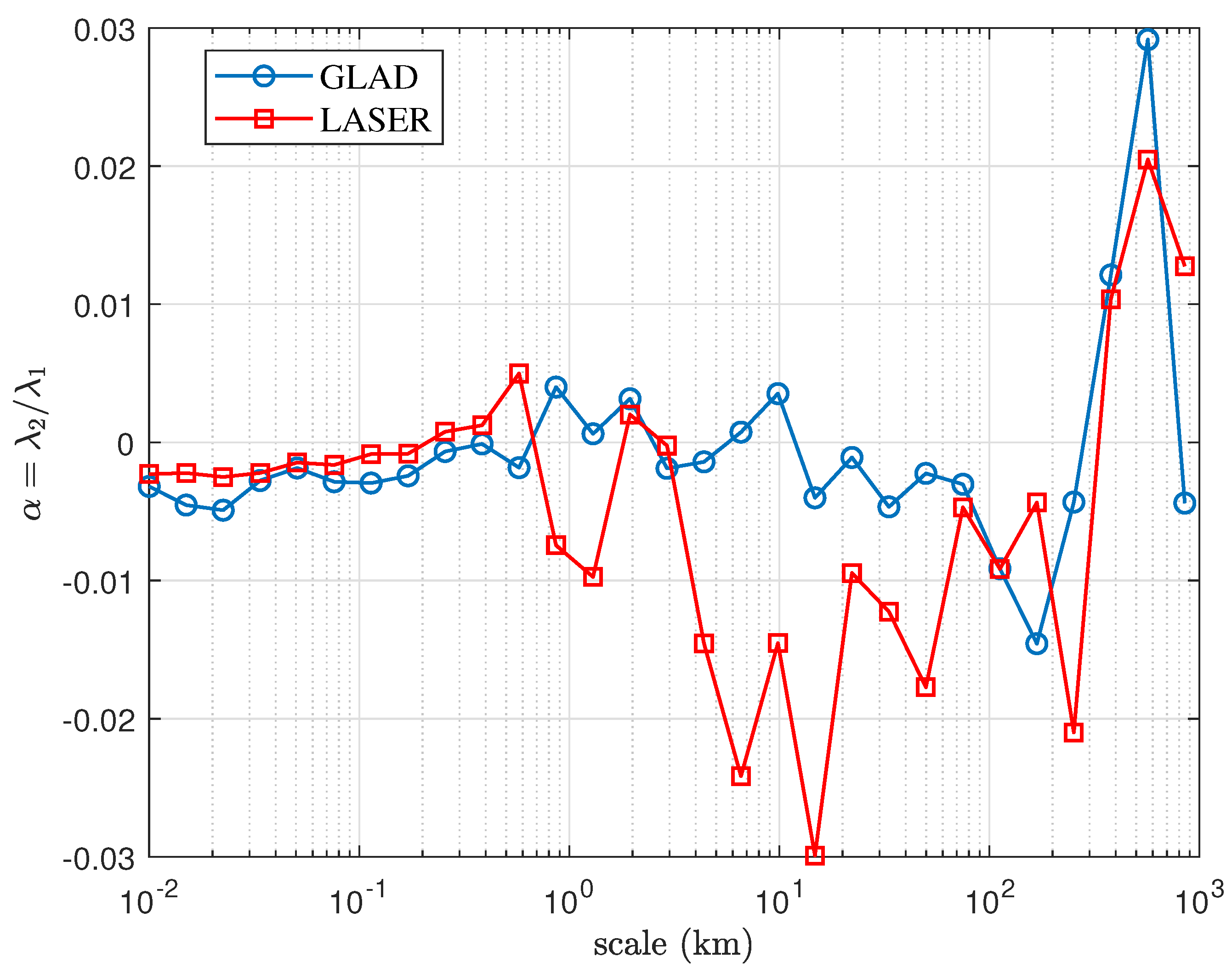
The above process can be carried out in other scales of , in GLAD and LASER. More fitting results are shown in Appendix C. Then we can get as a function of scale, which is shown in Figure 3. Details of data processing and error estimation are written in Appendix A and Appendix B, which will tell us that Figure 3 is reliable when the scale is above 3 km. We can find that is on the order of in general, and stays negative when the scale ranges from about 10 km to about 300 km. This range of scale is larger in LASER than in GLAD, and so does the amplitude of negative .
4. Discussion
Figure 3 shows that is negative (implying on average divergent flow) at most of the scales, with some positive (convergent flows) at scales around 1-10km. The negative is more prominent in LASER than in GLAD. This at least verifies that the surface flow is weakly compressible, as is small and non-zero, and may involve some patterns in 3D flows. Besides, compared with theories of 3D homogeneous isotropic turbulence [13] with (which may imply a positive )1, the negative implies the uniqueness of oceanic flow. We do not know the exact reason behind this negative , but we propose in the following sections two possible explanations.
4.1. Kinematics: Drifter Concentration Caused by Mesoscale Vortices and Surface Compressibility
Cressman et al. (2004) [14,15] analysed the motion of small particles on the surface of water in a square tank, and simulated the velocity distribution numerically. They claimed that surface flow is a compressible flow with low speed (lower than the speed of sound). Structures of source and sink will exist on the surface, as the motion is still 3D in essence. Particles will be trapped in narrow convergent regions (with negative 2D divergence of velocity), and be distribute around vortices with a larger scale.
For oceanic flows, the leading order vortices are mesoscale eddies (ranging from several km to several hundreds of km). It is possible that these mesoscale vortices are accompanied with narrow convergent fronts, so that the drifters will accumulate around these vortices [12]. Meanwhile, the vortices correspond to divergent regions due to mass conservation. This qualitative view agrees with the suggestion of divergence (negative ) at mesoscales ( km), with some suggestion of convergence (positive ) at submesoscale fronts ( km). We further speculate, that the negative alpha seen at even smaller scales may correspond to the divergent zones of Langmuir cells.
4.2. Dynamics: Weak Compressibility Caused by Ekman Pumping
Coriolis force is non-negligible for large scales in oceanic flows. The balance between Coriolis force and internal friction force is significant near the surface, resulting in the boundary layer between the ocean and the atmosphere, which is called the Ekman layer. Some contents in this section will use Vallis (2017) [1] as a reference.
For the Ekman layer on the surface of the ocean, friction at the bottom is zero (from definition), and wind stress will happen at the top. The z-component w of the velocity stays zero at the top, but non-zero at the bottom:
Here denotes the z-component of the curl, , where is the horizontal component of the velocity under geostrophic balance. The term represents the divergence of geostrophic transport, which is relatively small in (24).
Therefore, wind stress with a curl consistent with the rotation of the earth (i.e. positive curl in the northern hemisphere) will cause the up-welling and surface divergence, which is likely to contribute to the negative . The Gulf of Mexico is a region associated with negative wind stress curl on average [16], which could not explain the observed positive (divergence) at scales larger than km. However, this region is also subject to hurricanes, which are cyclones with a positive wind stress curl. In particular, the LASER experiment experienced a strong hurricane, which may explain the more negative detected in the LASER dataset.
5. Conclusions
We constructed a pure-strain model with a parameter to analyse the drifter data, where can reflect the existence of compressibility in a 2D flow, and the horizontal divergence asymmetry in 2D turbulence. We find that stays negative at the mesoscales, representing a divergent flow, and we conjecture that mesoscale eddies interspersed with convergent fronts or a wind stress with a cyclonic wind stress curl arising from hurricanes may explain this observed divergence.
This study analyzed two data sets, and our model better matches LASER than GLAD (shown in Appendix B). This difference may be caused by the difference in data volume, or our assumptions, such as homogeneity and isotropy, are better satisfied in LASER than in GLAD. The inhomogeneity and anisotropy in GLAD were already discussed in other studies [17].
A major caveat of this work is that we assumed the flow to be pure-strain; but oceanic flows are known to have comparably strong vorticity as well [18]. Thus, this strong assumption on our flow model may impact some of the results and conclusions. Also, our model is probably invalid when the velocity gradient tensor changes significantly with time, and the assumption of linearity is restrictive. Regardless, we provide an interesting and novel proof of concept for analyzing ocean observations, which is worthy of further investigation.
Author Contributions
Conceptualization, methodology, formal analysis, T. Z., J.-H. X. and D. B.; data processing: T. Z. and D. B.; writing—original draft preparation, T. Z.; writing—review and editing, T. Z., J.-H. X. and D. B. All authors have read and agreed to the published version of the manuscript.
Funding
T.Z. and J.-H.X. acknowledge financial support from the National Natural Science Foundation of China (NSFC) under grant numbers 12272006, 42361144844 and 12472219 and from the Laoshan Laboratory under grant numbers LSKJ202202000, LSKJ202300100. D.B. acknowledges financial support from the U.S. National Science Foundation under grant number NSF-OCE-2242110.
Data Availability Statement
The surface drifter data are available at https://data.gulfresearchinitiative.org/.
Acknowledgments
Conflicts of Interest
The authors declare no conflicts of interest.
Appendix A. Details of Data Processing
The data used in this research covers the time period from day 10 to day 52 in GLAD and LASER experiments. The positions (latitudes and longitudes) and velocities of the drifters are contained in the original data. Acceleration is computed by the central differencing scheme, and the time interval between neighbouring data points is 15 minutes originally. The actual used data takes 30 minutes as the time interval.
The p.d.f. of (defined by the first equals sign in (9)) is generated at different scales of (i.e. the distance between drifters). We choose a sequence as the representative scales in advance. This is a geometric sequence with a common ratio of , so that it is equidistant in the logarithmic coordinate and is consistent with a former study [5]. Meanwhile, we tolerate a relative error of when categorizing each actual into a certain , i.e. is considered on the scale of if and only if . Then almost all the data can be used without repetition when the scale is between the first and the last term of . The first term is set as m and the last term is about 852 km, so there are 29 terms of in total, all consistent with [5]. The examples in Figure 1, Figure 2 and Figure A1, where the scale is chosen as 33 km, correspond to to be precise.
As is mentioned in Section 2.3, we choose a sequence with a common difference of to represent different values of when generating the p.d.f. of . To obtain the p.d.f., we compute a discrete probability mass function (p.m.f.) of the event sequence , where . The extreme case will fall under the last interval. Divide the p.m.f. by , and we can get the p.d.f. for analysis. In the main text, is set as by default.
The function in Section 2.3 is also defined on discrete points . The derivative of can be defined by a discrete format with second-order accuracy, i.e.
Appendix B. Error Estimation of the Fitting
Appendix B.1. Noise in the Generated p.d.f.
We generated p.d.f. of from drifter data directly. But these functions are not smooth, and contain irregular oscillation, which is called noise. The existence of noise will reduce the effect and reliability of our fitting. Observation tells us that noise will probably decrease (i.e. Signal to Noise Ratio (SNR) will increase) as the scale and data volume increase. For instance, there are more valid drifters in LASER (956) than in GLAD (297), and accordingly, the p.d.f.s appear smoother in LASER than in GLAD.
Moreover, SNR will also increase when appropriately increases. An example is taken for 33 km in LASER, shown in Figure A1. Obvious oscillations can be seen when , and this phenomenon vanishes gradually as grows up. However, changes in will result in changes in the obtained , and the amplitude of this change also depends on the scale and data volume.
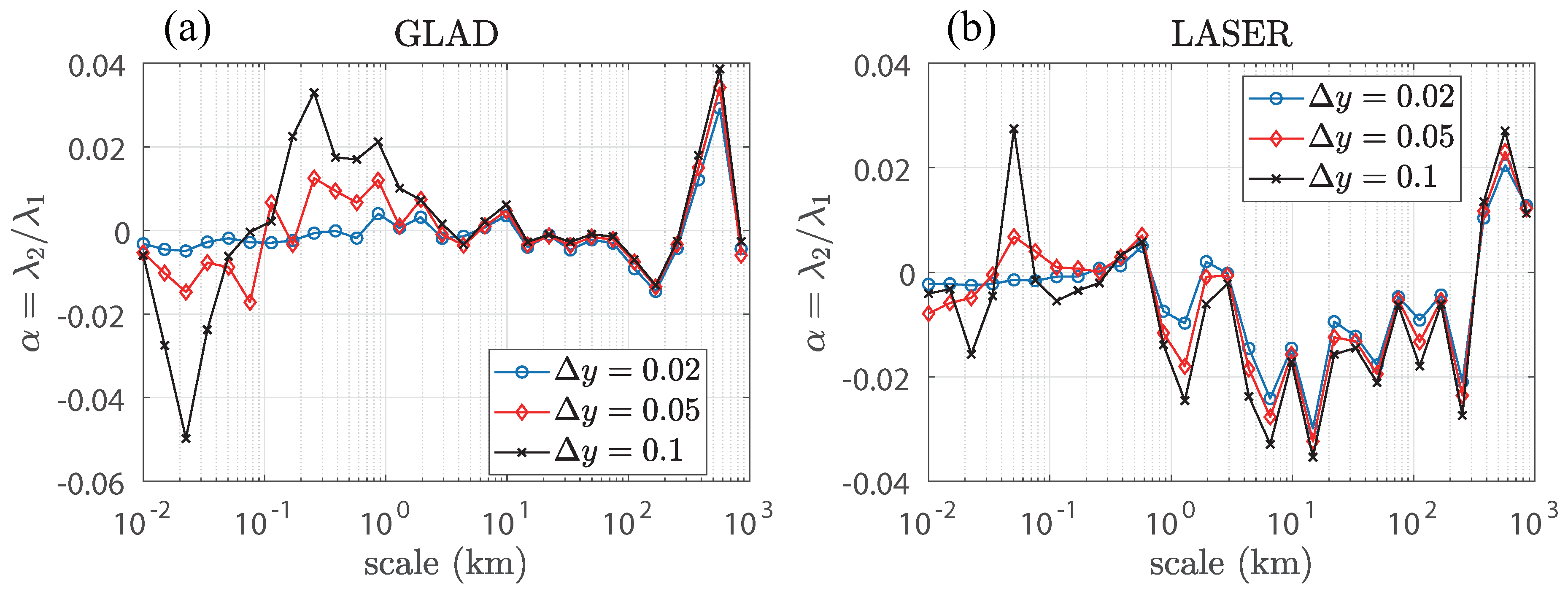
We can plot the - curves at different values of , which are shown in Figure A2. There should not be big changes in if our method is proper enough. According to Figure A2, small scales correspond to a bigger amplitude of change in and thus a lower reliability compared with the larger scales. The demarcation approximately locates at 3 km.
Figure A1.
Odd part of the p.d.f. and the fitting curve when equals (a) , (b) and (c) , at the scale around 33 km in LASER.
Figure A1.
Odd part of the p.d.f. and the fitting curve when equals (a) , (b) and (c) , at the scale around 33 km in LASER.
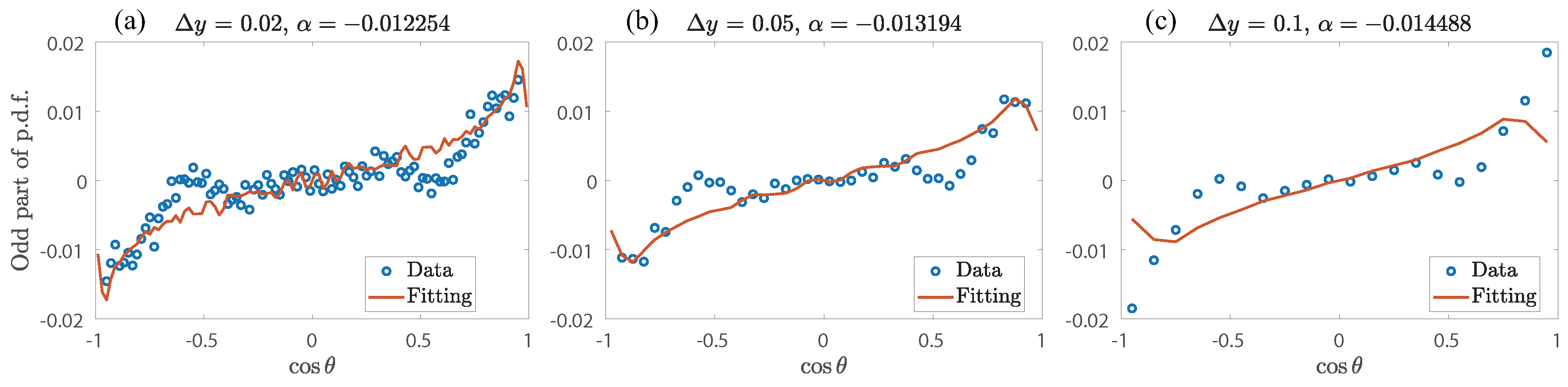
Figure A2.
The - curves at different values of in (a) GLAD and (b) LASER. The values of are set as , and , plotted in blue, red and black respectively.
Figure A2.
The - curves at different values of in (a) GLAD and (b) LASER. The values of are set as , and , plotted in blue, red and black respectively.
Appendix B.2. Root Mean Square Error
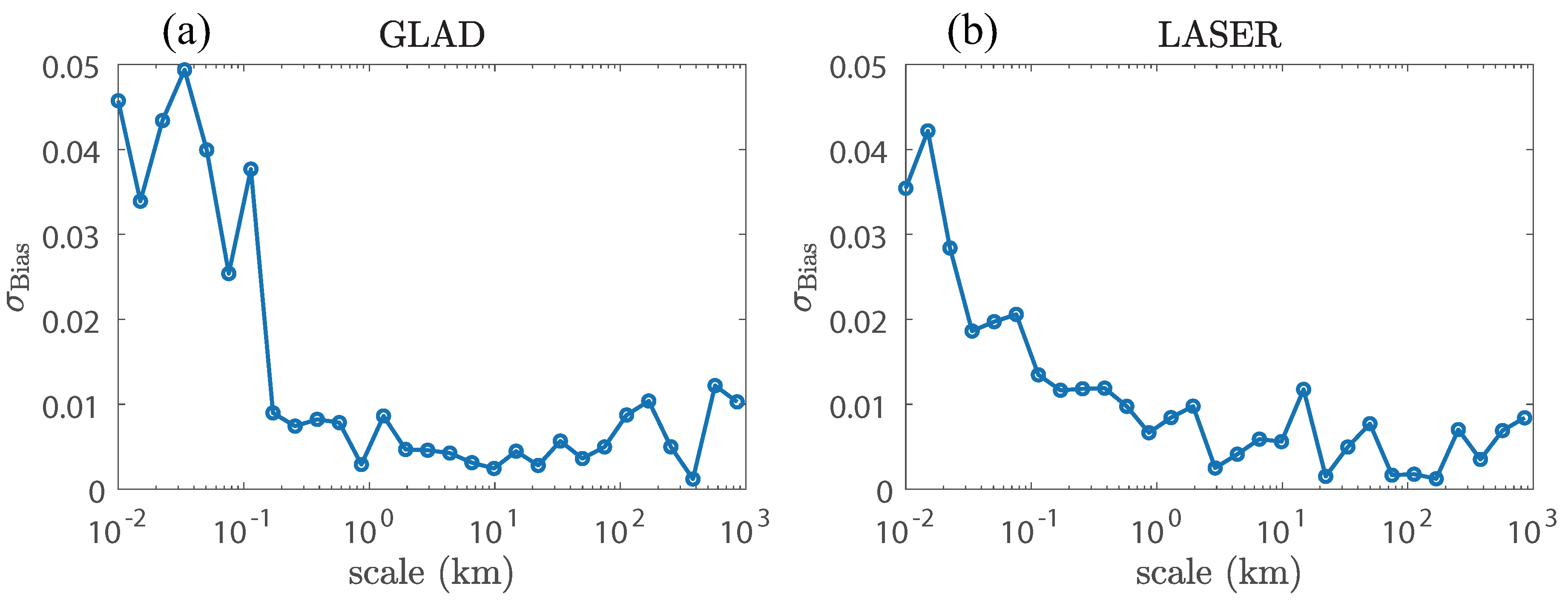
In the former section, We found that the fitting is effective and reliable at mesoscale and large scale. But we have not checked whether the fitting matches the p.d.f. well enough, and this is independent from the existence of noise. Therefore, we set to increase SNR, and define the bias of fitting as:
where denotes the number of data points when , and denote the odd part of the p.d.f. of and the fitting curve. Figure A3 shows the - curves. The value of reduces to a stable platform when the scale is over 500 m.
Figure A3.
- curves in (a) GLAD and (b) LASER.
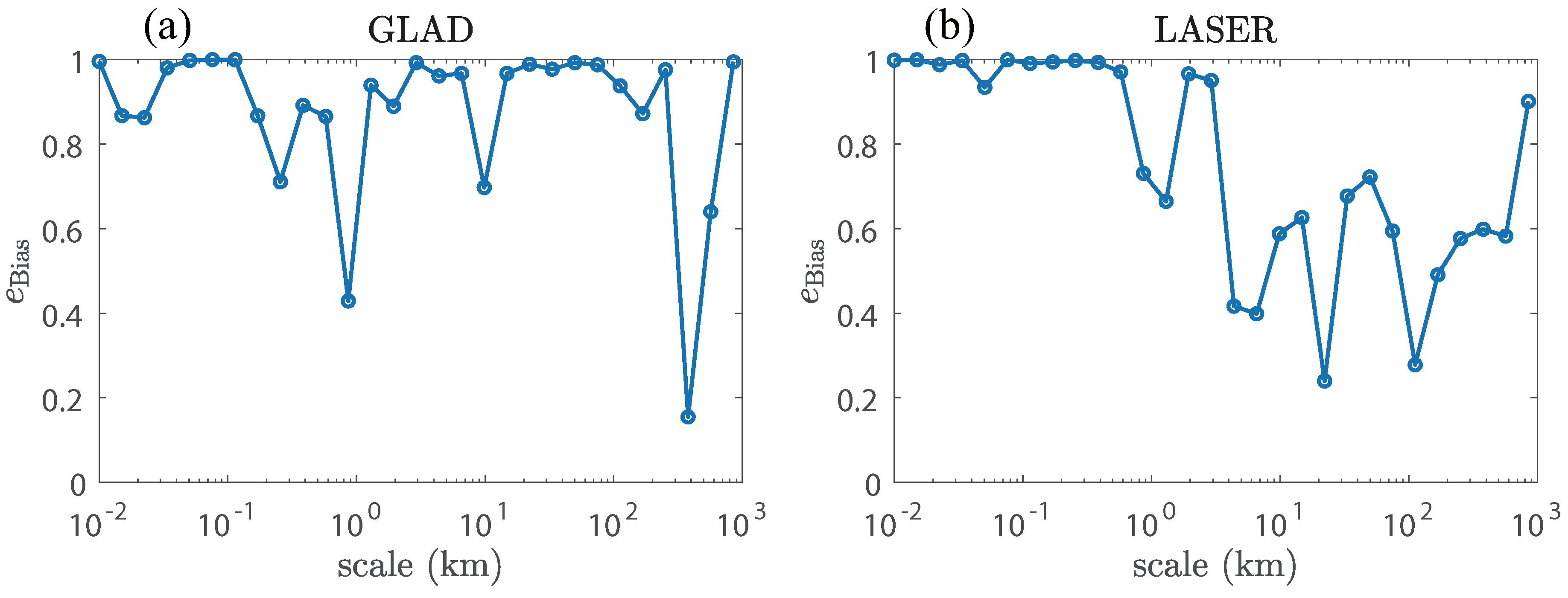
In addition, the amplitude of the odd part of the p.d.f. of will vary as the scale changes. A quantity describing the relative error needs to be introduced, i.e.
The - curves are shown in Figure A4. We can find that the fitting matches better in LASER than in GLAD, and the error is indeed smaller in larger scales (roughly larger than 3 km). The difference between the two data sets may be resulted by the difference of data volume, or GLAD is less likely to accord with our model.
Figure A4.
- curves in (a) GLAD and (b) LASER.
Appendix C. More Fitting Results
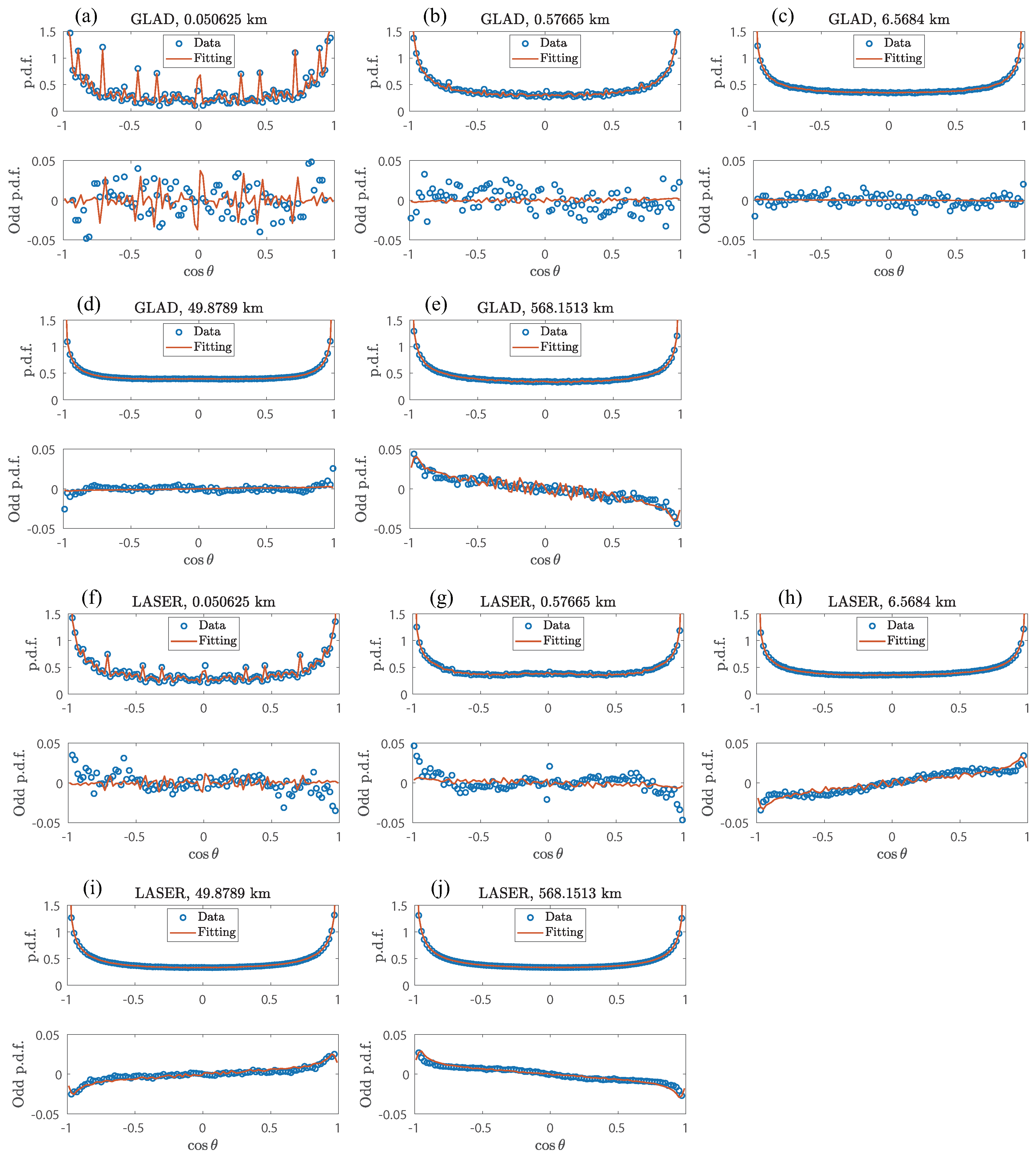
Here we select more fitting results in GLAD and LASER, as are shown in Figure A5. The value of is set as . In GLAD, obvious oscillations of data and the fitting curve appear when the scale is small (Figure A5(a)). The fitting curves are approximately horizontal at mesoscale (Figure A5(b)–(d)). This is consistent with the result that the amplitude of is smaller in GLAD than in LASER at mesoscale, as can be seen in Figure 3. Large scales have a better fitting result (Figure A5(e)). The oscillation of the fitting curve around in Figure A5(e) may be resulted by insufficient data volume. In LASER, oscillation is less obvious than in GLAD when the scale is small, while the curves appear horizontal and capture little features of the data (Figure A5(f)(g)). The fitting is fine for mesoscale and large scale (Figure A5(h)–(j)).
Figure A5.
Fitting results of p.d.f. of at different scales, using the data from (a)–(e) GLAD and (f)–(j) LASER. Five cases are shown here for each data set, which are at 51 m, 577 m, km, 50 km and 568 km respectively. Each single case contains two sub-figures, plotting the whole and the odd part of the p.d.f. (blue circles) and the fitting curve (red curve).
References
- Vallis, G.K. Atmospheric and oceanic fluid dynamics; Cambridge University Press, 2017.
- Vallis, G.K. Essentials of atmospheric and oceanic dynamics; Cambridge university press, 2019.
- Cho, J.Y.; Lindborg, E. Horizontal velocity structure functions in the upper troposphere and lower stratosphere: 1. Observations. Journal of Geophysical Research: Atmospheres 2001, 106, 10223–10232. [Google Scholar] [CrossRef]
- Qiu, B.; Nakano, T.; Chen, S.; Klein, P. Bi-directional energy cascades in the Pacific Ocean from equator to subarctic gyre. Geophysical Research Letters 2022, 49, e2022GL097713. [Google Scholar] [CrossRef]
- Balwada, D.; Xie, J.H.; Marino, R.; Feraco, F. Direct observational evidence of an oceanic dual kinetic energy cascade and its seasonality. Science Advances 2022, 8, eabq2566. [Google Scholar] [CrossRef] [PubMed]
- McWilliams, J.C. Submesoscale currents in the ocean. Proceedings of the Royal Society A: Mathematical, Physical and Engineering Sciences 2016, 472, 20160117. [Google Scholar] [CrossRef] [PubMed]
- Balwada, D.; LaCasce, J.H.; Speer, K.G. Scale-dependent distribution of kinetic energy from surface drifters in the Gulf of Mexico. Geophysical Research Letters 2016, 43, 10–856. [Google Scholar] [CrossRef]
- Ott, S.; Mann, J. An experimental investigation of the relative diffusion of particle pairs in three-dimensional turbulent flow. Journal of Fluid Mechanics 2000, 422, 207–223. [Google Scholar] [CrossRef]
- Gibert, M.; Xu, H.; Bodenschatz, E. Where do small, weakly inertial particles go in a turbulent flow? Journal of Fluid Mechanics 2012, 698, 160–167. [Google Scholar] [CrossRef]
- Solomon, T.; Tomas, S.; Warner, J. Chaotic mixing of immiscible impurities in a two-dimensional flow. Physics of Fluids 1998, 10, 342–350. [Google Scholar] [CrossRef]
- Poje, A.C.; Özgökmen, T.M.; Lipphardt Jr, B.L.; Haus, B.K.; Ryan, E.H.; Haza, A.C.; Jacobs, G.A.; Reniers, A.; Olascoaga, M.J.; Novelli, G.; others. Submesoscale dispersion in the vicinity of the Deepwater Horizon spill. Proceedings of the National Academy of Sciences 2014, 111, 12693–12698. [Google Scholar] [CrossRef] [PubMed]
- D’Asaro, E.A.; Shcherbina, A.Y.; Klymak, J.M.; Molemaker, J.; Novelli, G.; Guigand, C.M.; Haza, A.C.; Haus, B.K.; Ryan, E.H.; Jacobs, G.A.; others. Ocean convergence and the dispersion of flotsam. Proceedings of the National Academy of Sciences 2018, 115, 1162–1167. [Google Scholar] [CrossRef] [PubMed]
- Betchov, R. An inequality concerning the production of vorticity in isotropic turbulence. Journal of Fluid Mechanics 1956, 1, 497–504. [Google Scholar] [CrossRef]
- Cressman, J.R.; Goldburg, W.I.; Schumacher, J. Dispersion of tracer particles in a compressible flow. Europhysics Letters 2004, 66, 219. [Google Scholar] [CrossRef]
- Cressman, J.R.; Davoudi, J.; Goldburg, W.I.; Schumacher, J. Eulerian and Lagrangian studies in surface flow turbulence. New Journal of Physics 2004, 6, 53. [Google Scholar] [CrossRef]
- Yu, L. Sea surface exchanges of momentum, heat, and freshwater determined by satellite remote sensing. Encyclopedia of ocean sciences 2009, 2, 202–211. [Google Scholar]
- Huntley, H.S.; Lipphardt Jr, B.; Kirwan Jr, A. Anisotropy and inhomogeneity in drifter dispersion. Journal of Geophysical Research: Oceans 2019, 124, 8667–8682. [Google Scholar] [CrossRef]
- Balwada, D.; Xiao, Q.; Smith, S.; Abernathey, R.; Gray, A.R. Vertical fluxes conditioned on vorticity and strain reveal submesoscale ventilation. Journal of Physical Oceanography 2021, 51, 2883–2901. [Google Scholar] [CrossRef]
| 1 | Here refers to the eigenvalues of the symmetric part of the velocity gradient tensor. |
Figure 1.
Comparison between the actual p.d.f. of and eq.(15) in LASER, at the scale around 33 km.
Figure 1.
Comparison between the actual p.d.f. of and eq.(15) in LASER, at the scale around 33 km.
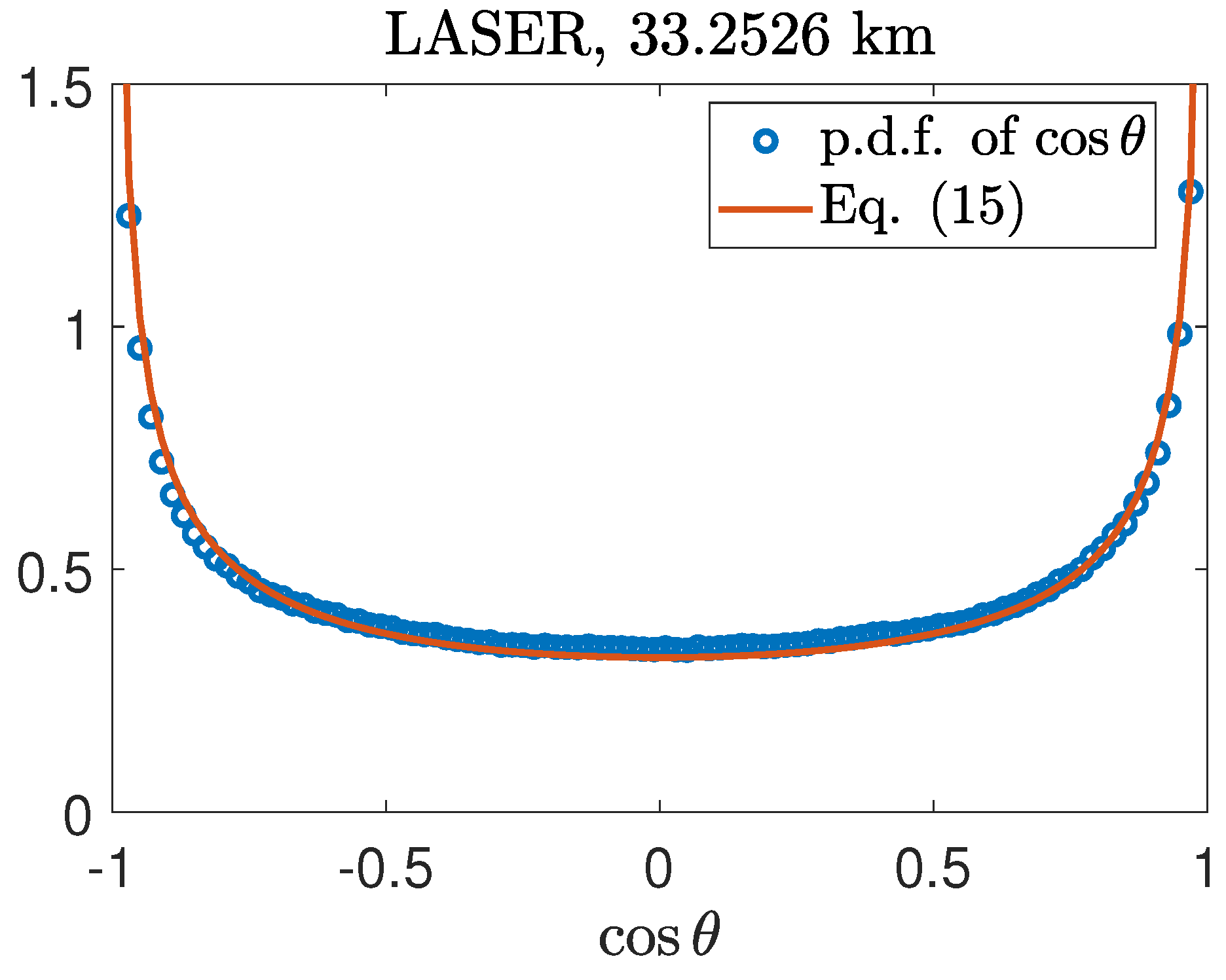
Figure 2.
Fitting process in LASER at the scale around 33km. (a) The even part of the p.d.f. of multiplied by , denoted as . (b) The derivative of q, using the discrete format in (A1). (c) The odd part of the p.d.f. of , denoted as , and its fitting curve , where is obtained by (23). Here, . (d) The comparison between the original data and fitting of p.d.f. of .
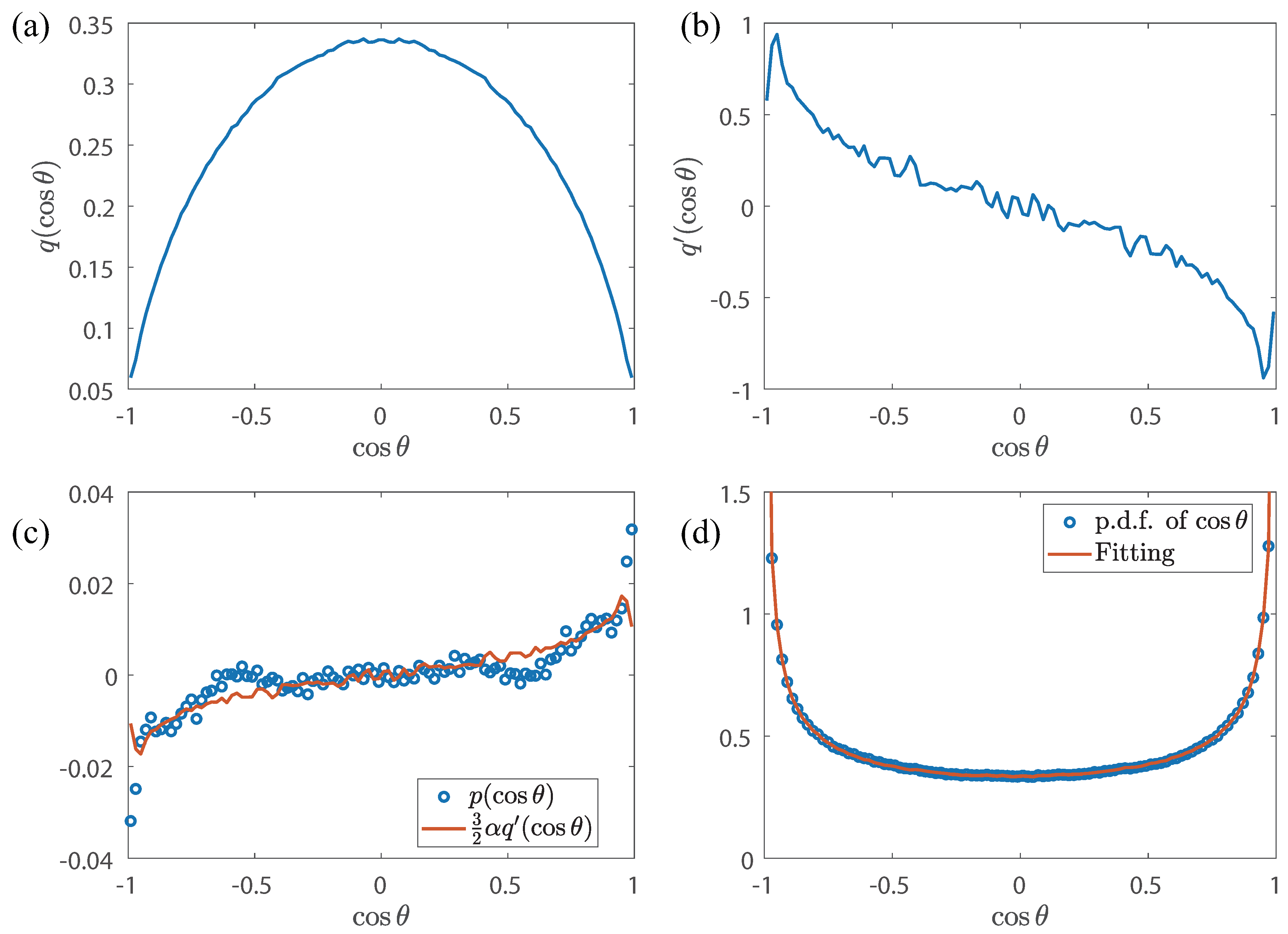
Figure 3.
The obtained - curve. Blue lines and red lines are used for GLAD and LASER, respectively.
Disclaimer/Publisher’s Note: The statements, opinions and data contained in all publications are solely those of the individual author(s) and contributor(s) and not of MDPI and/or the editor(s). MDPI and/or the editor(s) disclaim responsibility for any injury to people or property resulting from any ideas, methods, instructions or products referred to in the content. |
© 2024 by the authors. Licensee MDPI, Basel, Switzerland. This article is an open access article distributed under the terms and conditions of the Creative Commons Attribution (CC BY) license (http://creativecommons.org/licenses/by/4.0/).
Copyright: This open access article is published under a Creative Commons CC BY 4.0 license, which permit the free download, distribution, and reuse, provided that the author and preprint are cited in any reuse.


