
Submitted:
29 September 2025
Posted:
29 September 2025
You are already at the latest version
Abstract
This study examines the hydrodynamic conditions of the Gulf of California under three climate change scenarios—SSP1-2.6, SSP2-4.5, and SSP5-8.5—projected from 2015 to 2100 using the CNRM-CM6-1-HR global climate model. It evaluates changes in the annual and interannual variability of sea surface temperature (SST), ocean circulation, and key dynamic forcing mechanisms. The results reveal a general warming trend across the Gulf, characterized by an increased frequency of extreme heat events and a prolonged summer season. The Great Islands region emerges as the most resilient to climate change, with tidal forces remaining the dominant hydrodynamic driver. In contrast, the southern Gulf—from the mid-Gulf boundary to the entrance—is identified as the most vulnerable area, experiencing the highest number of extreme events and a more significant reduction in wind speed. This decline is particularly critical, as it affects essential oceanographic processes such as upwelling.
Keywords:
sea surface temperature
; ocean hydrodynamics
; climate change scenarios
; ocean heat waves
; ocean circulation
; dynamic ocean forcings
1. Introduction
Climate change (CC), defined as a modification of the climate directly or indirectly attributable to human activities [1] is part of a broader phenomenon known as global change (GC), which encompasses both biophysical and socioeconomic transformations of the Earth system [2,3]. The ocean plays a critical role in climate regulation, absorbing over 90% of the excess heat generated by greenhouse gases (GHGs) and approximately 30% of anthropogenic carbon dioxide (CO2) emissions [4,5,6]. These processes affect the ocean’s thermal structure [7], stratification [8], and circulation, which in turn have direct implications for marine biogeochemistry and ecosystems [9].
General Circulation Models (GCMs) are among the most advanced tools available for studying the climate system. These models integrate the physical, chemical, and biological processes governing the atmosphere, oceans, land surface, and cryosphere to simulate, understand, and project the behavior of the Earth’s climate. Developed by international governmental and non-governmental scientific institutions, GCMs have been evaluated and disseminated by the Intergovernmental Panel on Climate Change (IPCC) through various climate scenarios. These range from radiative forcing-based trajectories (RCPs) [10] to more comprehensive frameworks that incorporate socioeconomic dimensions (SSPs) [11]. Such scenarios allow for the analysis of climate change processes, including GHG emissions, and the challenges of mitigation and adaptation.
This study investigates the hydrodynamic conditions of the Gulf of California under different climate change scenarios. Specifically, the SSP1-2.6, SSP2-4.5, and SSP5-8.5 scenarios were applied using results of the CNRM-CM6-1-HR model to assess annual changes in interannual variability of sea surface temperature (SST) and the interaction of dynamic forcings within the Gulf.
CNRM-CM6-1-HR is a global climate model developed by the French National Centre for Meteorological Research (CNRM) and the European Centre for Advanced Research and Training in Scientific Computing (CERFACS). Its atmospheric component is based on the ARPEGE-Climat v6.3 model, while biospheric processes are simulated using the ISBA-CTRIP model. Limnological dynamics are handled by the FLake model. These components are integrated via SURFEX v8.0, enabling simulation of the land-atmosphere continuum.
For oceanic processes, the model incorporates NEMO (Nucleus for European Modelling of the Ocean) and GELATO for sea ice dynamics, both coupled through the OASIS-MCT module. The vertical resolution includes 91 levels for the atmosphere, 75 for the ocean, 14 for soil, and 12 for snow. The model also utilizes the configurable input/output XML server “XIOS,” developed by the Laboratory of Climate and Environmental Sciences at the Pierre-Simon Laplace Institute (IPSL/LSCE), to support high-performance, massively parallel simulations. Further details on the model configuration are available in Voldoire (2019) [12].
2. Materials and Methods
2.1. Study Area
The Gulf of California (Figure 1) is a region of significant ecological, fisheries, economic, and social importance [13,14,15]. It is currently facing a range of impacts associated with global environmental change, including the overexploitation of key fisheries such as sardine, mojarra, shark, sawfish, shrimp, oyster, and snapper [15]. Additionally, the Gulf receives substantial pollutant loads—including pesticides, domestic and industrial wastewater, and heavy metals and metalloids due to intensive agricultural, aquaculture, mining, and naval activities, as well as the presence of major coastal human settlements [16].
Since the first oceanographic expeditions by Sverdrup in 1939, the Gulf has been recognized as having a hydrographic and dynamic structure strongly influenced by seasonal and interannual variability, particularly by phenomena such as the El Niño–Southern Oscillation (ENSO) and the Pacific Decadal Oscillation (PDO) [17,18,19]. Sea surface temperature (SST) in the Gulf exhibits a distinct seasonal and regional pattern [20], through a time series analysis (1998–2022) of SST and chlorophyll-a (Chl-a), reported that the northern region—from the southern boundary of the Great Islands (GI) to the mouth of the Colorado River—is the coldest, with an average SST of 23.43 °C and eutrophic conditions (1.81 mg m−3). The central region showed an average SST of 24.59 °C and similarly eutrophic conditions (1.53 mg m−3). In contrast, the southern region was the warmest, with average SSTs ranging from 25.99 °C to 26.83 °C and exhibited oligotrophic conditions (0.37–0.95 mg m−3).
The hydrographic structure in the southern Gulf is particularly complex due to the exchange of water masses with the Pacific Ocean (PO) [21]. Seasonal latitudinal shifts of the Intertropical Convergence Zone (ITCZ) regulate the equatorial current system, which in turn influences the movement of Eastern Tropical Pacific (ETP) water masses near the Gulf’s entrance [22]. During March and April, the ITCZ is positioned near the equator, allowing the California Current to extend further south and limiting the inflow of surface and subsurface waters from the PO. Conversely, in September and October, the ITCZ shifts northward to approximately 10 °N, restricting the southward reach of the California Current and enabling PO waters to enter the Gulf—sometimes reaching as far north as the Great Islands region [23].
Thus, the ocean-atmosphere interactions in the PO regulate the inflow of water masses into the Gulf of California throughout the year. Consequently, the thermohaline structure at the Gulf’s mouth reflects that of the ETP, modified at the surface by evaporation [24]. In this context, salinity serves as a key tracer of surface circulation in the region [25].
Hydrodynamics in the Gulf of California is governed by three primary components: (1) forcing from the continuous interaction with the Pacific Ocean (PO), primarily through tides and ocean currents; (2) wind forcing at the surface; and (3) surface exchanges of heat and freshwater, representing the full spectrum of ocean-atmosphere interactions, along with the Gulf’s characteristic density gradients [26].
The Gulf exhibits a marked seasonal component in its surface circulation, primarily driven by wind regimes. During summer, southeasterly trade winds—originating from the Intertropical Convergence Zone (ITCZ) with average speeds of 5 m s−1—facilitate the inflow of Pacific waters through the eastern side of the Gulf’s mouth, promoting cyclonic circulation [27,28]. These winds also bring tropical storms into the region [29]. In contrast, during winter, strong northwesterly winds (8–12 m s−1), originating from the North American plains, induce anticyclonic surface circulation, effectively driving water out of the Gulf toward the Pacific [26,27,30,31,32]. These winds also trigger coastal upwelling along the eastern Gulf, a key mechanism for nutrient redistribution. Several studies [33,34,35] suggest that wind-driven upwelling systems may intensify under climate change, although the ecological consequences remain uncertain.
Kelvin wave signals associated with ENSO events propagate into the Gulf, influencing sea surface temperature (SST) and mean sea level [36,37]. According to Beck and Mahony (2018) [6], ENSO events may reach critical tipping points under future climate scenarios, potentially altering global and regional climate dynamics. The ecological impacts of ENSO in the Gulf are complex and species-specific [21,38]. The dominant tidal constituent in the Gulf is the M2 tide, which propagates as a Kelvin wave. Due to the Gulf’s permanent connection to the Pacific Ocean, a tidal co-oscillation occurs. Resonance conditions and the decreasing depth toward the northern Gulf result in one of the world’s largest tidal ranges (7–9 m) [39]. The Upper Gulf and the Great Islands region absorb over 70% of the incoming M2 energy, most of which is dissipated through bottom friction and turbulent mixing around the islands. Tidal residual currents significantly contribute to surface circulation and generate cyclonic motion that promotes upwelling on the western side of Tiburón Island, bringing cold, nutrient-rich waters to the surface and supporting a biologically productive region driven by astronomical forcing [39,40].
Lluch-Cota et al. (2010) [18], using projections based on the IPCC A1b scenario, reported that temperature variability in the Gulf is primarily driven by ENSO and PDO, with no sustained long–term trends in physical, chemical, or biological variables. However, Lluch-Belda et al. (2009) [41] identified a warming trend in SST since the early 1960s, while [42] reconstructed SST using observational and satellite data and found a slight cooling trend over the past 20–25 years. In adjacent oceanic regions, such as the eastern Mexican Pacific and the western coast of Baja California Sur, [43] applied statistical downscaling to RCP2.6, 4.5, 6.0, and 8.5 scenarios and projected a 1.68 °C increase in temperature and a 25% decline in net primary productivity, potentially reducing suitable habitat for Pacific sardine. Arellano & Rivas (2016) [35] projected a 1–4 °C temperature increase in the Gulf, deepening of the thermocline, and increased wind stress, leading to 30–250% increases in Chl-a concentrations during spring in the western Baja California Sur region. However, they concluded that intensified upwelling may not yield positive outcomes for ecosystems or fisheries.
López Martínez et al. (2023) [20] identified a warming trend in SST at an annual rate of 0.036 °C (0.73 °C over 20 years) and a decline in productivity at 0.012 mg m−3 per year (0.25 mg m−3 over 20 years). Their study also highlighted the close association between SST, Chl-a, and hydrodynamic structures such as filaments and eddies—features expected to become more prominent under climate change.
Hydrodynamic mechanisms play a vital role in fertilizing the Gulf through wind-driven upwelling, intense tidal mixing in the Great Islands region, and thermo-haline circulation that redistributes nutrients. Additionally, mesoscale cyclonic eddies have been identified as important fertilization mechanisms [44,45,46,47,48,49,50], contributing to the Gulf of California’s status as one of the most productive marine ecosystems in the world [13].
2.2. Hydrographic Analysis
2.2.1. Seasonal, Annual and Interannual Variability
The data for the SSP1-2.6, SSP2-4.5, and SSP5-8.5 scenarios were obtained from https://aims2.llnl.gov/ for projections generated using the CNRM-CM6-1-HR model. The dataset spans the period from 2015 to 2100 and includes the following variables: potential temperature, absolute salinity, zonal and meridional current velocities, and zonal and meridional wind speeds at 10 m above the surface. The data has a spatial resolution of 0.25 ° and a monthly temporal resolution. Using potential temperature and absolute salinity, seawater density was calculated with the gsw toolbox implemented in MATLAB, following the TEOS-10 standard (https://teos-10.org/).
To analyze the evolution of sea surface temperature (SST), a Fast Fourier Transform (FFT) was applied. This spectral analysis enabled the identification of dominant frequencies in SST variability, as well as the characteristic periods and cycles under different climate change scenarios [51].
Additionally, a Seasonal-Trend decomposition using LOESS (STL) was performed, following the methodology proposed by Cleveland et al (1990) [52]. The SST time series, , was decomposed into three main components: Trend (): representing long-term changes, Seasonal (): capturing regular cyclical patterns, and Residual (): encompassing interannual varia-bility and noise. This decomposition allowed for a clearer understanding of the under-lying dynamics and variability of SST in the Gulf of California under projected climate scenarios.
The first step is to obtain the detrended series (The first step is to obtain the detrended series () by eliminating seasonality. To do this the component must be subtracted from the original series. by eliminating seasonality. To do this the component must be subtracted from the original series.
Now the term will contain the trend and the residual, that is, the seasonally adjusted series. A LOESS is then applied, based on:
The weights in LOESS are obtained with a bicubic weight function of the form:
Where, is the temporal distance between point i and the center point t, d is the size of the smoothing window (e.g., 12 months in an annual series). Values closer to t receive more weight, and values further away receive less weight. Once the weights, , are calculated, the trend is estimated by fitting a local polynomial regression within the window . For each point t, the weighted regression equation is solved:
Equation five represents a local linear fit applied within each smoothing window using weighted least squares. The result of this fit is the estimated trend value at each time point t. Repeating this process across the entire time series yields a smoothed trend curve . This method effectively captures gradual changes in the data without imposing a predefined functional form, such as a straight line or fixed-degree polynomial.
To perform the STL decomposition, a seasonal window of 12 months was used to accurately capture the annual SST cycle. This ensures that the seasonal component reflects periodic variability without distorting the long-term trend. The residual component, which contains interannual and decadal oscillations, is particularly relevant for identifying signals associated with the El Niño–Southern Oscillation (ENSO) and the Pacific Decadal Oscillation (PDO).
Subsequently, a wavelet analysis was applied to the residual component using Python. This component is crucial, as it contains variability in timescales greater than two years, i.e., interannual variability. Unlike the FFT, wavelet analysis allows for the identification of both the timing and amplitude of dominant frequencies throughout the time series. This makes it a powerful tool for detecting non-stationary signals and temporal shifts in oceanographic processes. Wavelet analysis has been widely used to decompose and examine complex oceanographic phenomena across multiple temporal and spatial scales [53,54,55].
2.2.2. Analysis of Summer Duration in Future Scenarios
To evaluate changes in summer length based on sea surface temperature (SST), the methodology proposed by Peña-Ortiz et al. (2015) [56] was followed. To calculate and compare summer duration under the three climate change scenarios (SSP1-2.6, SSP2-4.5, and SSP5-8.5) in the Gulf of California, two temperature thresholds were defined: one for the onset of summer () and another for its end (). These thresholds correspond to the mean SST values for June and September, respectively, calculated from the full-time series.
A 30-day moving average was applied to the SST time series for each year to smooth short-term fluctuations. The start of summer was identified as the first day the smooth SST exceeded.
2.2.3. Extreme SST Events
The analysis of extreme events and the hydrodynamic assessment described below were conducted by dividing the study area into seven regions (Figure 1). López Martínez et al. (2023) [20] proposed a division of the Gulf of California into six bioregions based on a cluster analysis of sea surface temperature (SST) and chlorophyll-a concentrations. These variables are closely linked to mesoscale features such as eddies and filaments, which are visible manifestations of the prevailing hydrodynamic conditions [19]. For this reason, the present study adopted this regionalization framework.
However, a modification was made to the northern portion of the Gulf: The Upper Gulf of California was separated from the Great Islands Region. This adjustment was based on the recognition that inertial forces play a particularly significant role in the Great Islands area, warranting its distinction as a separate hydrodynamic zone.
From the trend component of the sea surface temperature (SST) time series, the 10th percentile (P10) and 90th percentile (P90) were calculated for each region and climate change scenario. Extreme cold events were defined as SST values below P10, while extreme heat events were defined as values exceeding P90. The frequency of these events was then computed for each decade to assess their temporal evolution and regional variability. This percentile-based approach is widely used in climate studies to detect trends in extreme events, as it avoids assumptions of normality in the data distribution [6,57], making it particularly suitable for analyzing non-linear and non-stationary climate signals.
2.3. Hydrodynamic Analysis
2.3.1. Dimensionless Numbers
To characterize the hydrodynamics of the Gulf of California under the SSP scenarios, three dimensionless numbers were calculated for each region: the Froude Number [58], the Wedderburn Number [59], and the Stress Number [60]. These parameters collectively allow for the identification of the dominant forcing mechanisms acting on the water body under study.
Equation (6) describes the momentum balance along the longitudinal axis (x), assuming a steady-state and irrotational flow. The use of dimensionless numbers provides a robust framework for comparing hydrodynamic regimes across regions and scenarios, independent of scale, and is particularly useful for assessing the relative influence of wind stress, buoyancy, and tidal forcing.
In Equation (6), the terms represent the inertial stress, while the term corresponds to the baroclinic pressure gradient. The term represents the sea surface elevation gradient, and accounts for frictional stresses due to vertical turbulent mixing. Here, x, y, and z denote the longitudinal, transverse, and vertical coordinate axes, respectively. The variables u and v are the fluid velocities in the x and y directions, g is the gravitational acceleration, is the water density, is the reference density, is the vertical turbulent viscosity coefficient, and is the sea surface height.
The dimensionless numbers—Froude, Wedderburn, and Stress—are derived from Equation (7) through dimensional analysis, allowing for the characterization of dominant hydrodynamic forcing mechanisms across different regions and climate scenarios.
2.3.2. Froude Number
The term in Equation (6) represent the inertial stresses, which can be scaled as , where U is the characteristic velocity and L is the characteristic length scale. The term represents the baroclinic pressure gradient, which can be scaled as or alternatively as , where H is the depth scale, is the density contrast (which may be vertical, longitudinal, or transverse), and is the reduced gravity.
From this scaling, the Froude number () is defined as:
The Froude number is a dimensionless parameter used in fluid dynamics to characterize the relative importance of inertial forces compared to gravitational (buoyancy) forces. In a two-layer stratified system, the effective gravitational force is given by the buoyancy term , and the internal Froude number [58] is expressed as:
Where U is the fluid velocity, is the reduced gravity, and is a representative length scale, which may correspond to the length or depth of the channel, bay, or gulf.
When: inertial forces dominate, indicating a predominantly turbulent flow regime. buoyancy forces dominate, and the flow is primarily governed by stratification and gravity. inertial and buoyancy forces are balanced, representing a transitional regime.
2.3.3. Wedderburn and Stress Numbers
The Wedderburn number (W) compares the relative importance of wind stress on the water column to the gravitational circulation of a stratified fluid [60]. It is defined as:
This number provides insight into whether the flow is primarily driven by internal dynamics (inertia) or by external forcing (wind stress).
When , external forces dominate, indicating a predominantly wind stress flow regime. inertial dominate. inertial and wind stress are balanced, representing a transitional regime.
3. Results
3.1. Annual and Interannual Variability of Surface Temperature in the Gulf of California
Spectral analysis (Figure 2) reveals that the annual signal is consistent across all SST time series under the different climate change scenarios analyzed. The results indicate a progressive increase in SST across all scenarios, with notable divergences emerging around the 2050s. Under the SSP5-8.5 scenario, a marked increase in the frequency of extreme warm events is observed, accompanied by a sharp decline in the occurrence of cold events.
This pattern suggests a shift in the thermal regime of the Gulf of California, with potential implications for ecosystem dynamics, stratification processes, and the frequency of climate-driven disturbances.
Figure 3 shows the time series for the different scenarios. In this figure (3a) is the “original series” (the result of the modeling of the different scenarios) of the monthly SST for the entire Gulf. This series allows a well-defined observation of annual variability. Differences between scenarios are also observed, with the high-emissions scenario exhibiting a progressive increase in sea surface temperature (SST) over time. Figure (3b) is the trend component (Long-Term). Long-term SST without the effect of seasonality or interannual variability. This allows us to observe a progressive increase trend in SST under any of the three scenarios analyzed. Figure (3c) is the seasonal component (Annual Cycle). This represents the seasonal variability of sea surface temperature (SST), characterized by a repetitive cycle that occurs annually. It allows us to identify a sinusoidal pattern that indicates warming in the summer months and cooling in the winter months. The amplitude of the seasonal cycle remains stable over time regardless of the scenario. Figure (3d) is the interannual and decadal variability component (Residual). It represents variability not explained by trend or seasonality, i.e., lower-frequency and noisy fluctuations. It contains signals of interannual (2-7 years, ENSO) and decadal (>10 years, PDO) variability. The amplitude of this signal is highly variable over time under any of the three scenarios.
The wavelet analysis results for SSP1-2.6, SSP2-4.5, and SSP5-8.5 scenarios (Figure 4) shows that the largest amplitudes are found in the 2- to 5-year period, which coincides with the El Niño event period. However, the main difference between the scenarios is when the largest amplitudes occur over time. For the SSP1-2.6 scenario, the largest amplitudes occur in the decades of 2020, 2040, and 2090, and a slight shift towards periods closer to 6-7 years of occurrence is also observed towards the end of the series, while for the SSP2-4.5 scenario, the largest amplitudes in sea surface temperature variability occur in the 2020s. There is a period with minimum amplitudes, followed by maximum amplitudes, from 2040 to 2090. For the SSP5-8.5 scenario, the period of maximum amplitudes remains below four years and exhibits continuity of up to a decade, which could indicate a longer duration of El Niño conditions.
The duration of days with temperatures similar to those of summers (Summer days) (Figure 5) shows an increase, averaging 80 days during 2020 and reaching 150 days in 2100 in the SSP1-2.6 scenario, 90 days during 2025, and 145 days in 2100 in the SSP2-4.5 scenario. For the SSP2-8.5 scenario in 2020, there are fewer than 80 summer days. Still, by 2100, it will reach more than 160 days.
The number of extreme heat events shows a consistent increase for the three scenarios analyzed, followed by an abrupt decrease by 2100 (Figure 5), while the number of extreme cold events exhibits a rise in 2020 and subsequently a decline, with a slight increase in 2080 in the SSP1-2.6 scenario (Figure 5).
3.2. Observed Trend in the Sea Surface Temperature and Direction of the Surface Current
Under the SSP1-2.6 scenario, the region with the highest warming rate is the Upper Gulf (0.0168 °C/year). In SSP2-4.5, the highest rate is found along the Southern Peninsula Coast and the Gulf entrance (0.0307 °C/year), while in SSP5-8.5, it shifts to the Central Gulf (0.0568 °C/year). Conversely, the lowest warming rates occur in the Southern and Oceanic Coast of Sinaloa (0.0152 °C/year) under SSP1-2.6, and in the Great Islands region under both SSP2-4.5 (0.0283 °C/year) and SSP5-8.5 (0.0504 °C/year). These results suggest relative thermal stability in the Great Islands region, while the Upper Gulf exhibits greater sensitivity to surface warming (Figure 6).
3.3. Observed Trend in the Speed and Direction of the Surface Current
All regions under the three climate change scenarios analyzed show a negative trend (Figure 7 and Figure 8), indicating a decrease in surface current velocity from 2015 to 2100 in the Gulf of California. The most evident decrease is in the central Gulf (26-28 °N) under the SSP5-8.5 scenario (-0.000509 m s−1 yr−1), followed by the Great Islands under the same scenario (-0.000243 m s−1 yr−1). The least pronounced decreases occur in the Upper Gulf under the SSP1-2.6 and SSP2-4.5 scenarios. The SSP5-8.5 scenario presents the most significant reductions in current speed across all regions. This suggests that currents could weaken significantly.
3.4. Observed Trend in Wind Speed and Direction at 10 m from the Surface
The monthly wind speeds for various regions within the Gulf of California under three climate change scenarios: SSP1-2.6, SSP2-4.5, and SSP5-8.5, shows negative trends in all regions (Figure 9 and Figure 10), indicating a gradual decrease in wind speed, except for the north-central coast of Sinaloa under the SSP5-8.5 scenario, where a slight increase is observed, and are positive for the Upper Gulf region under any scenario. The most pronounced reductions are observed along the southern coast of the peninsula and at the entrance to the Gulf, especially under the SSP2-4.5 and SSP5-8.5 scenarios. It is worth noting that the trends are statistically significant. These results indicate that climate change has a differential impact on wind dynamics in each region of the Gulf of California.
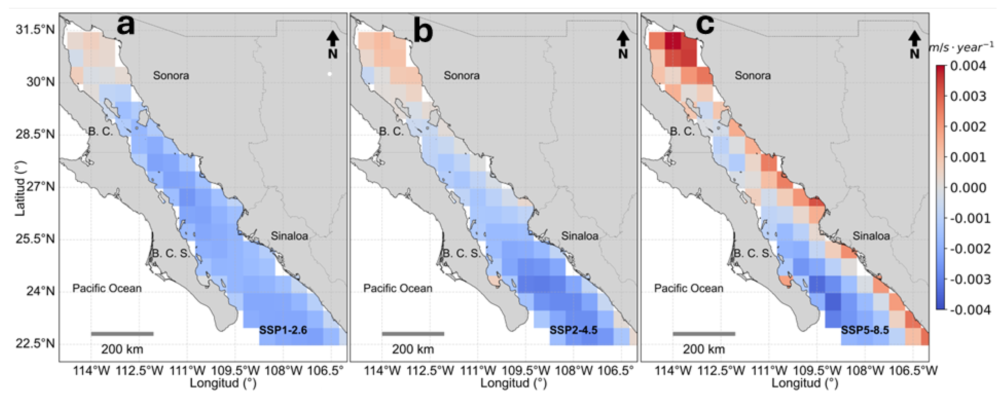
The Figure 11 shows the rate of change in speed per year (m s−1 year−1) for all regions under each of the SSP scenarios. When the scenario is low to medium emissions the exchange rate shows an increase in the region of the Upper Gulf and a decrease from the south of the GI to the mouth of the Gulf. For the SSP5-8.5 high emissions scenario, an increase in wind speed is observed along the entire eastern coast of the Gulf. To the Southwest of the Gulf the negative exchange rate remains as in the other scenarios.
3.5. Relative Comparison Between Efforts
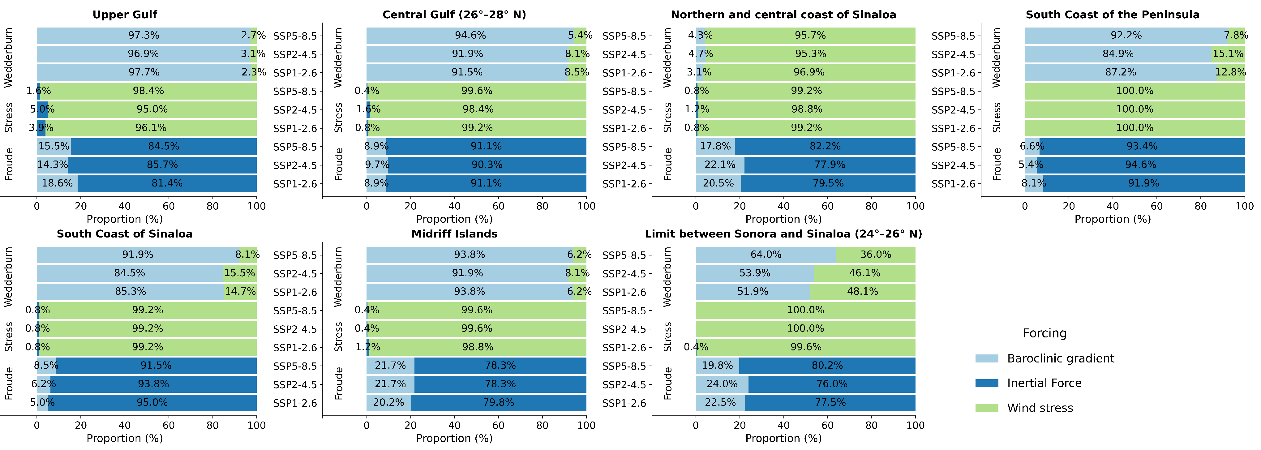
Within the Gulf of California, seasonal hydrographic conditions exhibit well-defined summer and winter regimes, each governed by distinct physical forcings. The summer period was delineated as July through October, while winter encompassed December through March. Under these seasonal frameworks, the relative contribution of various dynamic forcings was assessed using dimensionless numbers.
For each region and climate scenario, the dominance of specific forcings was quantified by calculating the proportion of monthly observations in which a given force prevailed. For instance, in the case of the Froude number (), a total of 344 monthly observations were analyzed. Instances where inertial forces dominated () and where baroclinic pressure gradients prevailed () were counted separately. These counts were then normalized to yield percentage values representing the seasonal dominance of each forcing mechanism. This approach enabled a comparative assessment of dynamic regimes across regions and scenarios, highlighting seasonal variability in the governing physical processes (see Figure 12 and 13).
The dimensionless Froude number () serves as a diagnostic metric to evaluate the relative dominance between inertial forces and baroclinic pressure gradients. Values of greater than 1 indicate a regime where inertial forces prevail, whereas values below 1 suggest dominance of baroclinic forcing.
Analysis across all climate change scenarios reveals a consistent pattern: inertial forces dominate throughout the Gulf of California during both summer and winter seasons. However, two exceptions were identified—namely, the southern coastal region of the Baja California Peninsula and the entrance to the Gulf—where baroclinic gradients exert greater influence during the summer months. In these regions, the seasonal transition leads to a reversal in dominance, with inertial forces regaining prevalence during the winter.
A noteworthy finding is the enhanced dominance of inertial forces over baroclinic pressure gradients during the winter season, particularly under the SSP2-4.5 and SSP5-8.5 climate scenarios. This trend suggests that as the climate forcing intensifies—from a moderate to a high-emission scenario—the frequency of inertial dominance increases across all regions of the Gulf of California during winter.
This behavior may be attributed to stronger wind forcing and reduced stratification under cooler conditions, which amplify inertial responses in the circulation dynamics. The progressive shift toward inertial dominance under more extreme scenarios highlights the sensitivity of regional hydrography to climate-induced changes in atmospheric and oceanic forcing mechanisms.
During the summer season, although inertial forces continue to dominate over baroclinic pressure gradients across most regions of the Gulf of California, their relative dominance decreases progressively from the conservative (SSP1-2.6) to the extreme (SSP5-8.5) climate scenario. Concurrently, the influence of the baroclinic gradient increases. This trend is particularly evident in the southern coastal region of the Baja California Peninsula and at the Gulf’s entrance, where baroclinic forcing becomes increasingly dominant under more extreme scenarios.
The dimensionless Wedderburn number (W) was used to assess the relative importance of wind stress versus baroclinic pressure gradients. Across all three climate scenarios, results indicate that baroclinic forcing dominates over wind stress in both summer and winter for the Upper Gulf, the Great Islands region, the Central Gulf (26°–28° N), the southern Gulf near the Sonora–Sinaloa boundary, and the southern oceanic coast of Sinaloa. In contrast, the north-central coastal region of Sinaloa exhibits a persistent dominance of wind stress over baroclinic forcing under all scenarios. However, this dominance weakens progressively from SSP1-2.6 to SSP5-8.5, in both summer and winter, suggesting a growing influence of baroclinic processes in this region under intensified climate forcing.
In contrast to the general pattern observed throughout the Gulf of California, the southern coastal region of the Baja California Peninsula and the Gulf’s entrance exhibit a distinct seasonal reversal in forcing dominance. During summer, wind stress prevails over baroclinic pressure gradients; however, its dominance diminishes progressively from the conservative SSP1-2.6 scenario to the more extreme SSP5-8.5 scenario. Conversely, during winter, baroclinic forcing becomes dominant in these regions, with its influence intensifying under increasingly extreme climate scenarios.
The dimensionless Stress number was employed to evaluate the relative importance of inertial forces versus wind stress. Across all regions and under all climate scenarios analyzed, wind stress consistently dominates over inertial forcing during both summer and winter. This persistent dominance underscores the critical role of wind-driven dynamics in shaping the circulation patterns of the Gulf of California, regardless of seasonal or climatic variability.
Figure 12.
Proportion of forcings during summer by region and scenario.
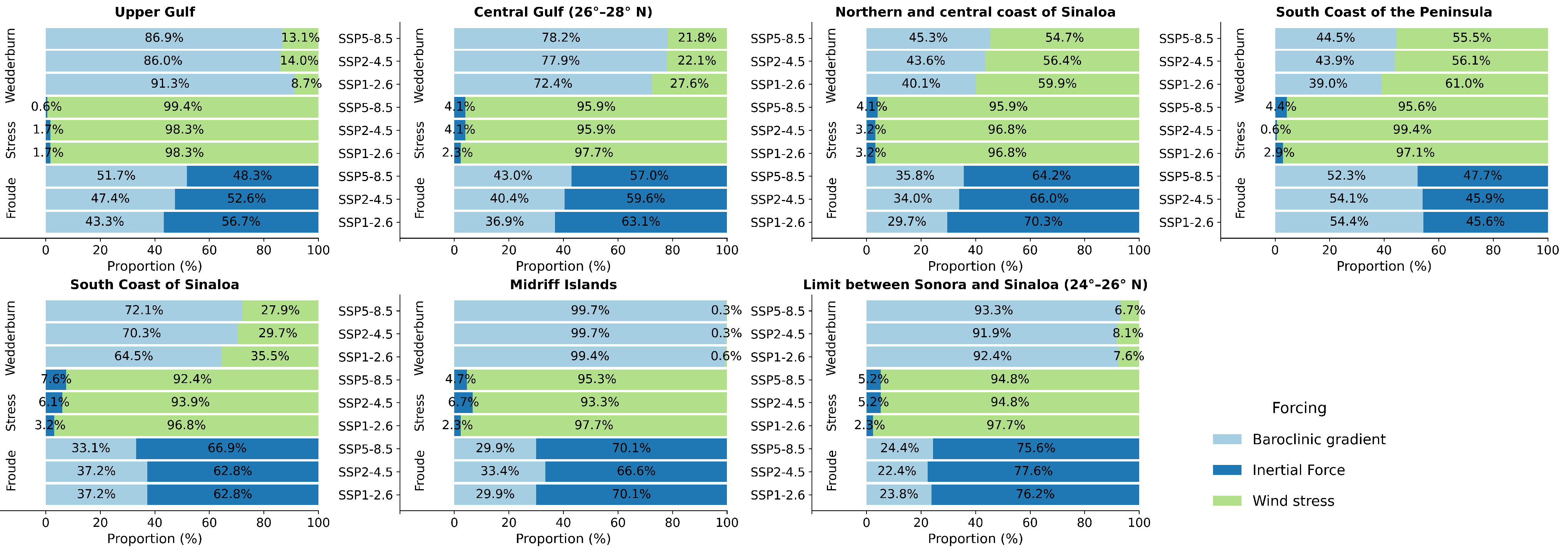
Figure 13.
Proportion of forcings during winter by region and scenario.
4. Discussion
Spectral analysis using the Fast Fourier Transform (FFT) reveals that dominant frequencies in sea surface temperature (SST) variability correspond to annual and interannual cycles, while lower-frequency components are associated with seasonal and semiannual patterns. Across all three climate change scenarios evaluated using the CNRM-CM6-1-HR model (SSP1-2.6, SSP2-4.5, and SSP5-8.5), the spectral structure remains consistent at seasonal time scales, suggesting that greenhouse gas emissions exert limited influence on short-term periodicity (i.e., 1-year and 0.5-year cycles). In contrast, frequencies associated with variability beyond two years exhibit scenario-dependent differences, indicating that long-term SST variability may be more sensitive to anthropogenic forcing or more challenging to simulate accurately in general circulation models (GCMs). This is consistent with findings by [5], who reported substantial inter-model variability in the representation of El Niño–Southern Oscillation (ENSO) dynamics across more than 30 CMIP models. Seasonal-Trend Decomposition using Loess (STL) further supports the presence of a persistent upward trend in SST throughout the Gulf of California. The seasonal component retains its amplitude and periodicity, indicating that the rate of increase in mean monthly SST during both winter and summer remains relatively stable over time. To assess the implications of warming on seasonal duration, STL results were complemented by quantifying the number of months per year with SST exceeding 26 °C. This analysis reveals a clear extension of the summer season from 2015 to 2100, consistent with broader hemispheric trends reported by Peña-Ortiz et al., (2015) Pena-Ortiz et al. [56] and Park et al., (2023) Park et al. [61].
Wavelet analysis highlights the presence of low-frequency variability associated with ENSO events under different climate scenarios. Under SSP1-2.6, El Niño signals are discrete and temporally bounded, whereas under SSP2-4.5 and SSP5-8.5, the signal persists for extended periods—sometimes exceeding a decade. These findings align with previous studies [61] that emphasize the sensitivity of ENSO amplitude and du-ration to emissions scenarios and model configuration. Expanding the analysis to addi-tional regions using consistent GCM-scenario combinations could help constrain uncertainties in model projections. Despite limitations in temporal and spatial resolution, the CNRM-CM6-1-HR model demonstrates robust performance in reproducing regional SST seasonality and capturing low-frequency climate phenomena such as ENSO.
Overall, the study identifies a consistent increase in SST across the Gulf of Cali-fornia under all evaluated scenarios. The magnitude of warming is scenario-dependent, with SSP5-8.5 exhibiting the most pronounced increases. This supports the hypothesis that moderate mitigation efforts (e.g., SSP2-4.5) may slow SST rise in the latter half of the century, whereas limited mitigation (SSP5-8.5) leads to sustained warming through 2100 [62].
Analysis of extreme SST events reveals a rising frequency of extreme heat events and a declining occurrence of extreme cold events across all regions of the Gulf throughout the 21st century. The SSP5-8.5 scenario shows the most significant increase in extreme heat events beginning in the 2050s, suggesting that under high-emissions conditions, such events will become both more frequent and more intense. Conversely, extreme cold events are projected to nearly disappear by the end of the century, particularly in the central and southern Gulf, underscoring the vulnerability of these regions to climate change. These results are consistent with global trends reported by Wang et al. (2024) [63], who documented a widespread decline in extreme cold events across tropical and subtropical oceans.
Regions with the highest projected frequency of extreme heat events under all scenarios include the southern coast of the Baja California Peninsula, the entrance to the Gulf of California, and the southern and oceanic coasts of Sinaloa. Under SSP5-8.5, up to 38 extreme heat events are projected during the 2090–2100 decade in these areas. Such events may have profound ecological consequences, including coral bleaching, disruption of commercial fisheries, and shifts in marine species distributions [64].
Analysis of the 10th and 90th percentile values of sea surface temperature (SST) reveals that the most vulnerable regions to thermal increases include the southern coast of the Baja California Peninsula, the entrance to the Gulf of California, the southern oceanic coast of Sinaloa, and the central Gulf. Under the SSP5-8.5 scenario, these regions are projected to experience SST increases exceeding 4.9 °C. Such warming trends pose a significant risk to marine ecosystems, particularly for species with narrow thermal tolerance ranges critical for physiological processes such as development and reproduction. These findings are consistent with previous studies [22,65], which documented increasing SST trends over recent decades. However, the present analysis suggests that under high-emissions scenarios, the magnitude of warming may surpass earlier estimates, with potential implications for ocean circulation and vertical stratification.
Surface current velocity is projected to decline across all regions of the Gulf, with the most pronounced reductions occurring in the central Gulf and the Great Islands region under SSP5-8.5 scenario. This weakening of circulation may impair nutrient transport and primary productivity, potentially disrupting trophic dynamics and ecosystem stability. The Gulf’s circulation exhibits a seasonal inversion in its northern sector, characterized by cyclonic flow from June to September and anticyclonic flow from November to April, both with average velocities near 0.35 m s−1. These seasonal patterns have been successfully reproduced by numerical models in previous studies [30,32].
Wind forcing, represented by 10 m wind speed, shows a general declining trend across most regions, although regional anomalies are present. For example, a slight increase in wind speed is projected along the north-central coast of Sinaloa under SSP5-8.5, potentially driven by enhanced pressure gradients. In contrast, the overall reduction in wind speed across the Gulf suggests a weakening of vertical mixing processes, which may promote increased stratification of the water column. Wind patterns in the Gulf are strongly seasonal, modulated by shifts in atmospheric pressure systems and the complex topography of the mainland and the Baja California Peninsula [66]. From November to April, northwesterly winds dominate at speeds of 8–12 m s−1, while southeasterly winds prevail during summer at approximately 5 m s−1 [28]. Northwesterly winds induce Ekman transport to the right of the wind vector, facilitating upwelling along the eastern coast—one of the primary mechanisms for nutrient redistribution in the region.
While several studies [33,34,35] have proposed that wind-driven coastal upwelling systems may intensify under climate change due to enhanced thermal gradients and atmospheric circulation, the findings of this study diverge from that perspective. Specifically, Arellano & Rivas (2019) [35] reported an intensification of upwelling events in the Gulf of California (GoC) linked to climate change. In contrast, our results suggest that an increase in wind intensity does not directly lead to a greater development of wind-driven upwelling systems. Although stronger winds enhance Ekman transport—by removing more surface water and accelerating surface currents—this effect is not consistently observed across all analyzed climate scenarios. This interpretation aligns with observations by Robinson (2016) [67], who documented a significant decline in upwelling intensity off the western coast of the Baja California Peninsula during the 2014–2015 period, attributed to anomalously warm SSTs and reduced wind forcing in the California Current System.
Furthermore, SST anomalies in the GoC have been shown to influence precipitation patterns in northwestern Mexico and the southwestern United States of America (USA). Mo & Higgins (2008)[68] and Kim et al. (2005) [69] found that warm SSTs in the northern GoC enhance monsoonal rainfall, while cold SSTs suppress it. Mo & Juang (2003) [70] noted that this influence is primarily confined to northwestern Mexico. In contrast, Mitchell et al. (2002) [71] reported that intense monsoonal precipitation in the south-western USA is associated with SSTs exceeding 29 °C in the GoC during the July–September period.
The present study identifies a consistent rise in SST and an increase in the number of days with summer-like thermal conditions, which may imply a longer monsoon season or an increase in rainfall events. However, it is important to consider that global warming is also associated with a higher frequency and intensity of tropical cyclones [72] demonstrated that approximately 50% of Gulf moisture surge events are linked to tropical cyclones. These events can induce SST cooling through wave-driven mixing and increased cloud cover, which reduces incoming solar radiation and net surface heat flux [68,72]. Nevertheless, such episodic cooling events are insufficient to offset the long-term warming trend observed in the Gulf, particularly under high-emissions scenarios.
5. Conclusions
The analysis of dimensionless numbers reveals progressive shifts in the physical processes governing the Gulf of California (GoC) under increasing greenhouse gas emissions. Across all scenarios (SSP1-2.6, SSP2-4.5, SSP5-8.5), the GoC is projected to evolve into a warmer, less dynamic, and more stratified system. This transformation is driven by declining wind stress, reduced surface current velocities, and enhanced baroclinic gradients.
Regions such as the Upper Gulf and the southern coast of the Baja California Peninsula emerge as particularly vulnerable. In these areas, wind stress—identified as the dominant forcing mechanism—exhibits a statistically significant negative trend, which corresponds with observed reductions in surface current speeds. In contrast, regions like the Great Islands and the Northern Gulf, located within the subtropical zone, are primarily influenced by tidal forcing. Tides in these regions act as a key dissipative mechanism, promoting vertical mixing and contributing to system resilience.
Surface current velocities are projected to decline throughout the Gulf, with the most pronounced reductions occurring in the central basin under the SSP5-8.5 scenario. This weakening of circulation may impair nutrient transport and primary productivity, with cascading effects on marine food webs. The northern Gulf maintains its seasonal inversion pattern—cyclonic circulation from June to September and anticyclonic from November to April—with average velocities near 0.35 m s−1. However, the projected reduction in flow intensity raises questions about its impact on the formation and renewal of Gulf of California Water (GCW) in the Upper Gulf, a topic warranting further investigation.
Wind forcing, represented by 10-m wind speed, also shows a general downward trend, albeit with regional variability. For instance, a slight increase is projected along the north-central coast of Sinaloa under SSP5-8.5, potentially linked to intensified pressure gradients during specific seasons. Nevertheless, the overall decline in wind speed suggests reduced vertical mixing and enhanced stratification of the water column.
All three scenarios analyzed using the CNRM-CM6-1-HR model project a warming of the surface layer in the GoC. The annual SST variability signal remains dominant across scenarios, but summers are expected to lengthen significantly, with surface temperatures exceeding 27 °C for durations ranging from 8 to 12 consecutive months. Low-frequency processes such as El Niño (2–7 years) continue to dominate interannual SST variability, with amplitudes between 0.5 and 0.9 °C. These anomalies may persist for nearly a decade, indicating prolonged El Niño-like conditions under future climate regimes.
As climate forcing intensifies, the Gulf’s hydrodynamics are expected to transition toward a more stratified circulation regime. While the dominant forcing mechanisms remain regionally consistent, their relative influence shifts across scenarios. Baroclinic gradients gain prominence relative to inertial and wind stresses, particularly under high-emissions pathways.
Latitude plays a critical role in modulating regional resilience. The Great Gulf Islands region demonstrates the highest resilience, primarily due to the dominance of tidal forcing, which sustains vertical mixing and system stability. Conversely, the Upper Gulf—despite its higher latitude—is less resilient due to its dependence on wind stress, which is projected to weaken.
The southern coast of the Baja California Peninsula and the north-central coast of Sinaloa are identified as the most vulnerable regions. In both cases, wind stress is the primary forcing mechanism, and its projected decline under climate change increases susceptibility to warming, stratification, and associated ecological impacts.
Author Contributions
MRR: Conceptualization, Methodology, Software, Validation, Formal analysis, Investigation, Data curation, Visualization, Writing—original draft preparation, Project administration. DASL: Methodology, Writing—review and editing, Supervision.
Funding
This research received no external funding.
Data Availability Statement
All data used in this study are publicly available and can be freely downloaded from the CMIP6 database at: https://aims2.llnl.gov/search/cmip6
Acknowledgments
The authors express their gratitude to Posgrado en Ciencias del Mar y Limnología, UNAM, for supporting this work, and to CONACYT for PhD fellowship to MRR (No. CVU 745610). This study was supported by UNAM through Instituto de Ciencias del Mar y Limnología (grants 144, 145), DGAPA-PAPIIT project IG100421 “Análisis de las interacciones entre aguas continentales y marinas en el Golfo de California bajo el enfoque de la fuente al mar como base para su gestión sustentable,” and DGTIC project LANCAD-UNAM-DGTIC-346 “Modelación numérica tridimensional baroclínica del Golfo de México, Golfo de California y Mar Caribe y modelos de transporte.”
Conflicts of Interest
The authors declare no conflicts of interest.
References
- UN. United Nations Framework Convention on Climate Change, UNFCCC. Technical Report 1, UN, 1992.
- Álvarez-Lires, M.; Arias-Correa, A.; Lorenzo-Rial, M.; Serrallé-Marzoa, F. Educación para la sustentabilidad: cambio global y acidificación Oceánica. Formación universitaria 2017, 10, 89–102. [Google Scholar] [CrossRef]
- Escoto Castillo, A.; Sánchez Peña, L.; Gachuz Delgado, S. Trayectorias Socioeconómicas Compartidas (SSP): nuevas maneras de comprender el cambio climático y social. Estudios demográficos y urbanos 2017, 32, 669–693. [Google Scholar] [CrossRef]
- Change, I.C. The physical science basis. IPCC Sixth Assessment Report 2013. [Google Scholar]
- Cheng, L.; Zhang, L.; Wang, Y.; Canadell, J.; Chiew, F.; Beringer, J.; Li, L.; Miralles, D.; Piao, S.; Zhang, Y. Recent increases in terrestrial carbon uptake at little cost to the water cycle. Nature Communications 2017, 8, 110. [Google Scholar] [CrossRef]
- Beck, S.; Mahony, M. The IPCC and the new map of science and politics. Wiley Interdisciplinary Reviews: Climate Change 2018, 9, e547. [Google Scholar] [CrossRef]
- Hoegh-Guldberg, O.; Mumby, P.; Hooten, A.; Steneck, R.; Greenfield, P.; Gomez, E.; Harvell, C.; Sale, P.; Edwards, A.; Caldeira, K.; et al. Coral reefs under rapid climate change and ocean acidification. Science 2007, 318, 1737–1742. [Google Scholar] [CrossRef]
- Li, G.; Cheng, L.; Zhu, J.; Trenberth, K.; Mann, M.; Abraham, J. Increasing ocean stratification over the past half-century. Nature Climate Change 2020, 10, 1116–1123. [Google Scholar] [CrossRef]
- Libes, S. Introduction to Marine Biogeochemistry; Academic Press, 2011.
- Moss, R.; Edmonds, J.; Hibbard, K.; Manning, M.; Rose, S.; van Vuuren, D.; Carter, T.; Emori, S.; Kainuma, M.; Kram, T.; et al. The next generation of scenarios for climate change research and assessment. Nature 2010, 463, 747–756. [Google Scholar] [CrossRef]
- O’Neill, B.; Lawrence, P.; Ren, X. Coupling integrated assessment and earth system models: concepts and an application to land use change. In Proceedings of the AGU Fall Meeting Abstracts, 2016, Vol. 2016, pp. GC31A–1109.
- Voldoire, A.; Saint-Martin, D.; Sénési, S.; Decharme, B.; Alias, A.; Chevallier, M.; Colin, J.; Guérémy, J.; Michou, M.; Moine, M.; et al. Evaluation of CMIP6 deck experiments with CNRM-CM6-1. Journal of Advances in Modeling Earth Systems 2019, 11, 2177–2213. [Google Scholar] [CrossRef]
- Lara-Lara, J.; Arenas-Fuentes, V.; Bazán-Guzmán, C.; Díaz-Castañeda, V.; Escobar-Briones, E.; García-Abad, M.; Gaxiola-Castro, G.; Robles-Jarero, G.; Sosa-Avalos, R.; Soto-González, L.; et al. Los ecosistemas marinos. Capital Natural de México 2008, 1, 135–159. [Google Scholar]
- Arreguín-Sánchez, F.; Arcos-Huitrón, E. La pesca en México: estado de la explotación y uso de los ecosistemas. Hidrobiológica 2011, 21, 431–462. [Google Scholar]
- Arreguín-Sánchez, F.; del Monte-Luna, P.; Zetina-Rejón, M.; Albáñez-Lucero, M. The Gulf of California large marine ecosystem: fisheries and other natural resources. Environmental Development 2017, 22, 71–77. [Google Scholar] [CrossRef]
- Páez-Osuna, F.; Álvarez-Borrego, S.; Ruiz-Fernández, A.; García-Hernández, J.; Jara-Marini, M.; Bergés-Tiznado, M.; Piñón-Gimate, A.; Alonso-Rodríguez, R.; Soto-Jiménez, M.; Frías-Espericueta, M.; et al. Environmental status of the Gulf of California: a pollution review. Earth-Science Reviews 2017, 166, 181–205. [Google Scholar] [CrossRef]
- Emilsson, I. Oceanografía físico-química del Golfo de California. Lecture Notes in Physical Oceanography 1991. [Google Scholar]
- Lluch-Cota, S.; Parés-Sierra, A.; Magaña-Rueda, V.; Arreguín-Sánchez, F.; Bazzino, G.; Herrera-Cervantes, H.; Lluch-Belda, D. Changing climate in the Gulf of California. Progress in Oceanography 2010, 87, 114–126. [Google Scholar] [CrossRef]
- Páez-Osuna, F.; Sanchez-Cabeza, J.; Ruiz-Fernández, A.; Alonso-Rodríguez, R.; Piñón-Gimate, A.; Cardoso-Mohedano, J.; Flores-Verdugo, F.; Carballo, J.; Cisneros-Mata, M.; Álvarez-Borrego, S. Environmental status of the Gulf of California: A review of responses to climate change and climate variability. Earth-Science Reviews 2016, 162, 253–268. [Google Scholar] [CrossRef]
- López Martínez, J.; Farach Espinoza, E.; Herrera Cervantes, H.; García Morales, R. Long-term variability in sea surface temperature and chlorophyll a concentration in the Gulf of California. Remote Sensing 2023, 15, 4088. [Google Scholar] [CrossRef]
- Torres-Martínez, C.; Monreal-Gómez, M.; Coria-Monter, E.; Salas-de León, D.; Durán-Campos, E.; Merino-Ibarra, M. Three-dimensional distribution of nutrients and phytoplankton biomass in a semi-enclosed region of the Gulf of California during different ENSO phases. Botanica Marina 2025, 68. [Google Scholar] [CrossRef]
- Lavín, M.; Castro, R.; Beier, E.; Cabrera, C.; Godínez, V.; Amador-Buenrostro, A. Surface circulation in the Gulf of California in summer from surface drifters and satellite images (2004–2006). Journal of Geophysical Research: Oceans 2014, 119, 4278–4290. [Google Scholar] [CrossRef]
- Álvarez-Borrego, S.; Schwartzlose, R. Water masses of the Gulf of California. Ciencias Marinas 1979, 6, 43–63. [Google Scholar] [CrossRef]
- Soto-Mardones, L.; Marinone, S.; Parés-Sierra, A. Time and spatial variability of sea surface temperature in the Gulf of California. Ciencias Marinas 1999, 25, 1–30. [Google Scholar] [CrossRef]
- Portela, E.; Beier, E.; Barton, E.; Castro, R.; Godínez, V.; Palacios-Hernández, E.; Fiedler, P.; Sánchez-Velasco, L.; Trasviña, A. Water masses and circulation in the tropical Pacific off central Mexico and surrounding areas. Journal of Physical Oceanography 2016, 46, 3069–3081. [Google Scholar] [CrossRef]
- Marinone, S. A three-dimensional model of the mean and seasonal circulation of the Gulf of California. Journal of Geophysical Research: Oceans 2003, 108. [Google Scholar] [CrossRef]
- Beier, E. A numerical investigation of the annual variability in the Gulf of California. Journal of physical oceanography 1997, 27, 615–632. [Google Scholar] [CrossRef]
- Roden, G. Oceanographic and meteorological aspects of the Gulf of California. Pacific Science 1958, 12, 21–47. [Google Scholar]
- Douglas, M.; Maddox, R.; Howard, K.; Reyes, S. The mexican monsoon. Journal of Climate 1993, pp. 1665–1677. [CrossRef]
- Lavín, M.; Durazo, R.; Palacios, E.; Argote, M.; Carrillo, L. Lagrangian observations of the circulation in the northern Gulf of California. Journal of Physical Oceanography 1997, 27, 2298–2305. [Google Scholar] [CrossRef]
- Beier, E.; Ripa, P. Seasonal gyres in the northern Gulf of California. Journal of Physical Oceanography 1999, 29, 305–311. [Google Scholar] [CrossRef]
- Palacios-Hernández, E.; Beier, E.; Lavín, M.; Ripa, P. The effect of the seasonal variation of stratification on the circulation of the northern Gulf of California. Journal of Physical Oceanography 2002, 32, 705–728. [Google Scholar] [CrossRef]
- Sydeman, W.; García-Reyes, M.; Schoeman, D.; Rykaczewski, R.; Thompson, S.; Black, B.; Bograd, S. Climate change and wind intensification in coastal upwelling ecosystems. Science 2014, 345, 77–80. [Google Scholar] [CrossRef]
- Bakun, A.; Black, B.; Bograd, S.; Garcia-Reyes, M.; Miller, A.; Rykaczewski, R.; Sydeman, W. Anticipated effects of climate change on coastal upwelling ecosystems. Current Climate Change Reports 2015, 1, 85–93. [Google Scholar] [CrossRef]
- Arellano, B.; Rivas, D. Coastal upwelling will intensify along the Baja California coast under climate change by mid-21st century: Insights from a GCM-nested physical-NPZD coupled numerical ocean model. Journal of Marine Systems 2019, 199, 103207. [Google Scholar] [CrossRef]
- Herrera-Cervantes, H.; Lluch-Cota, D.; Lluch-Cota, S.; Gutiérrez-de Velasco Sanromán, G. The ENSO signature in sea-surface temperature in the Gulf of California. Journal of Marine Research 2007, 65, 589–605. [Google Scholar] [CrossRef]
- Herrera-Cervantes, H.; Lluch-Cota, S.; Lluch-Cota, D.; Gutiérrez de Velasco Sanromán, G.; Lluch-Belda, D. ENSO influence on satellite-derived chlorophyll trends in the Gulf of California. Atmósfera 2010, 23, 253–262. [Google Scholar]
- Sánchez Velasco, L.; Godinez, V.; Ruvalcaba-Aroche, E.; Márquez-Artavia, A.; Beier, E.; Barton, E.; Jimenez-Rosemberg, P. Larval Fish Habitats and Deoxygenation in the Northern Limit of the Oxygen Minimum Zone off Mexico. In Proceedings of the AGU Fall Meeting 2019. AGU, 2019. [CrossRef]
- Salas-de León, D.; Carbajal-Pérez, N.; Monreal-Gómez, M.; Barrientos-MacGregor, G. Residual circulation and tidal stress in the Gulf of California. Journal of Geophysical Research: Oceans 2003, 108. [Google Scholar] [CrossRef]
- Marinone, S.; Lavín, M. Mareas y corrientes residuales en el Golfo de California. Contribuciones a la Oceanografía Física en México. Monografía 1997, 3, 113–139. [Google Scholar]
- Lluch-Belda, D.; del Monte-Luna, P.; Lluch-Cota, S. 20th century variability in Gulf of California SST. CalCOFI Reports 2009, 50. [Google Scholar]
- Lluch-Cota, S.; Tripp-Valdéz, M.; Lluch-Cota, D.; Lluch-Belda, D.; Verbesselt, J.; Herrera-Cervantes, H.; Bautista-Romero, J. Recent trends in sea surface temperature off Mexico. Atmósfera 2013, 26, 537–546. [Google Scholar] [CrossRef]
- Petatan-Ramirez, D.; Ojeda-Ruiz, M.; Sánchez-Velasco, L.; Rivas, D.; Reyes-Bonilla, H.; Cruz-Piñón, G.; Morzaria-Luna, H.; Cisneros-Montemayor, A.; Cheung, W.; Salvadeo, C. Potential changes in the distribution of suitable habitat for Pacific sardine (Sardinops sagax) under climate change scenarios. Deep Sea Research Part II: Topical Studies in Oceanography 2019, 169, 104632. [Google Scholar] [CrossRef]
- Sánchez-Velasco, L.; Lavín, M.; Jiménez-Rosenberg, S.; Godínez, V. Preferred larval fish habitat in a frontal zone of the northern Gulf of California during the early cyclonic phase of the seasonal circulation (June 2008). Journal of Marine Systems 2014, 129, 368–380. [Google Scholar] [CrossRef]
- Sánchez-Velasco, L.; Lavín, M.; Jiménez-Rosenberg, S.; Godínez, V.; Santamaría-del Angel, E.; Hernández-Becerril, D. Three-dimensional distribution of fish larvae in a cyclonic eddy in the Gulf of California during the summer. Deep Sea Research Part I: Oceanographic Research Papers 2013, 75, 39–51. [Google Scholar] [CrossRef]
- Coria-Monter, E.; Monreal-Gómez, M.; Salas-de León, D.; Aldeco-Ramírez, J.; Merino-Ibarra, M. Differential distribution of diatoms and dinoflagellates in a cyclonic eddy confined in the Bay of La Paz, Gulf of California. Journal of Geophysical Research: Oceans 2014, 119, 6258–6268. [Google Scholar] [CrossRef]
- Coria-Monter, E.; Monreal-Gómez, M.; Salas de León, D.; Durán-Campos, E.; Merino-Ibarra, M. Wind driven nutrient and subsurface chlorophyll-a enhancement in the Bay of La Paz, Gulf of California. Estuarine, Coastal and Shelf Science 2017, 196, 290–300. [Google Scholar] [CrossRef]
- Duran-Campos, E.; Salas-de León, D.; Monreal-Gómez, M.; Aldeco-Ramírez, J.; Coria-Monter, E. Differential zooplankton aggregation due to relative vorticity in a semi-enclosed bay. Estuarine, Coastal and Shelf Science 2015, 164, 10–18. [Google Scholar] [CrossRef]
- Durán-Campos, E.; Monreal-Gómez, M.; Salas de León, D.; Coria-Monter, E. Zooplankton functional groups in a dipole eddy in a coastal region of the southern Gulf of California. Regional Studies in Marine Science 2019, 28, 100588. [Google Scholar] [CrossRef]
- Durán-Campos, E.; Monreal-Gómez, M.; Salas de León, D.; Coria-Monter, E. Impact of a dipole on the phytoplankton community in a semi-enclosed basin of the southern Gulf of California, Mexico. Oceanologia 2019, 61, 331–340. [Google Scholar] [CrossRef]
- Rojo-Garibaldi, B.; Salas-de León, D.; Sánchez, N.; Monreal-Gómez, M. Hurricanes in the Gulf of Mexico and the Caribbean Sea and their relationship with sunspots. Journal of Atmospheric and Solar-Terrestrial Physics 2016, 148, 48–52. [Google Scholar] [CrossRef]
- Cleveland, R.; Cleveland, W.; McRae, J.; Terpenning, I. STL: A seasonal-trend decomposition. J. of Stat. 1990, 6, 3–73. [Google Scholar]
- Thomas, E.; Joseph, I.; Abraham, N. Wavelet analysis of annual rainfall over Kerala and sunspot number. New astronomy 2023, 98, 101944. [Google Scholar] [CrossRef]
- erán, B.; Recalde Mosquera, S.; Navarro Hernández, J.; Rozo Celemin, A.; Córdova Aguilar, J. Relación de la Corriente de Cromwell e índices ENOS en el Pacífico ecuatorial entre 1993 y 2017. Boletín Científico CIOH 2020.
- Durán-Campos, E.; Salas-de León, D.; Coria-Monter, E.; Monreal-Gómez, M.; Aldeco-Ramírez, J.; Quiroz-Martinez, B. ENSO effects in the southern Gulf of California estimated from satellite data. Continental Shelf Research 2023, 266, 105084. [Google Scholar] [CrossRef]
- Peña-Ortiz, C.; Barriopedro, D.; García-Herrera, R. Multidecadal variability of the summer length in Europe. Journal of Climate 2015, 28, 5375–5388. [Google Scholar] [CrossRef]
- Alsefri, M.; Sudell, M.; García-Fiñana, M.; Kolamunnage-Dona, R. Bayesian joint modelling of longitudinal and time to event data: a methodological review. BMC medical research methodology 2020, 20, 94. [Google Scholar] [CrossRef]
- Kundu, P.; Cohen, I.; Dowling, D. Fluid Mechanics; Elsevier, 206.
- Monismith, S. An experimental study of the upwelling response of stratified reservoirs to surface shear stress. Journal of Fluid Mechanics 1986, 171, 407–439. [Google Scholar] [CrossRef]
- Tenorio-Fernandez, L.; Valle-Levinson, A.; Gomez-Valdes, J. Subtidal hydrodynamics in a tropical lagoon: A dimensionless numbers approach. Estuarine, Coastal and Shelf Science 2018, 200, 449–459. [Google Scholar] [CrossRef]
- Park, J.; Schloesser, F.; Timmermann, A.; Choudhury, D.; Lee, J.; Nellikkattil, A. Future sea-level projections with a coupled atmosphere-ocean-ice-sheet model. Nature Communications 2023, 14, 636. [Google Scholar] [CrossRef] [PubMed]
- Kikstra, J.; Nicholls, Z.; Smith, C.; Lewis, J.; Lamboll, R.; Byers, E.; Sandstad, M.; Meinshausen, M.; Gidden, M.; Rogelj, J.; et al. The IPCC Sixth Assessment Report WGIII climate assessment of mitigation pathways: from emissions to global temperatures. Geoscientific Model Development 2022, pp. 9075–9109. [CrossRef]
- Wang, X.; Woolway, R.; Shi, K.; Qin, B.; Zhang, Y. Lake cold spells are declining worldwide. Geophysical Research Letters 2024, 51, e2024GL111300. [Google Scholar] [CrossRef]
- Walther, G.; Post, E.; Convey, P.; Menzel, A.; Parmesan, C.; Beebee, T.; Fromentin, J.; Hoegh-Guldberg, O.; Bairlein, F. Ecological responses to recent climate change. Nature 2002, 416, 389–395. [Google Scholar] [CrossRef]
- Ayala-Bocos, A.; Reyes-Bonilla, H.; Calderón-Aguilera, L.; Herrero-Perezrul, M.; González-Espinosa, P. Proyección de cambios en la temperatura superficial del mar del Golfo de California y efectos sobre la abundancia y distribución de especies arrecifales. Revista Ciencias Marinas y Costeras 2016, 8, 29–40. [Google Scholar] [CrossRef]
- Lavín, M.; Marinone, S. An overview of the physical oceanography of the Gulf of California. Nonlinear Processes in Geophysical Fluid Dynamics: A tribute to the scientific work of Pedro Ripa 2003, pp. 173–204.
- Robinson, C. Evolution of the 2014–2015 sea surface temperature warming in the central west coast of Baja California, Mexico, recorded by remote sensing. Geophysical Research Letters 2016, 43, 7066–7071. [Google Scholar] [CrossRef]
- Mo, K.; Higgins, R. Relationships between sea surface temperatures in the Gulf of California and surge events. Journal of climate 2008, 21, 4312–4325. [Google Scholar] [CrossRef]
- Kim, J.; Farrara, J.; Roads, J. The effects of the Gulf of California SSTs on warm-season rainfall in the southwestern United States and northwestern Mexico: A regional model study. Journal of climate 2005, 18, 4970–4992. [Google Scholar] [CrossRef]
- Mo, K.; Juang, H. Influence of sea surface temperature anomalies in the Gulf of California on North American monsoon rainfall. Journal of Geophysical Research: Atmospheres 2003, 108. [Google Scholar] [CrossRef]
- Mitchell, D.; Ivanova, D.; Rabin, R.; Brown, T.; Redmond, K. Gulf of California sea surface temperatures and the North American monsoon: Mechanistic implications from observations. Journal of Climate 2002, 15, 2261–2281. [Google Scholar] [CrossRef]
- Higgins, R.; Shi, W. Dominant factors responsible for interannual variability of the summer monsoon in the southwestern United States. Journal of Climate 2000, 13, 759–776. [Google Scholar] [CrossRef]
Figure 1.
Regionalization used for the Gulf of California. The Mexican states of Sinaloa, Sonora, Baja California (B.C.), and Baja California Sur (B.C.S.) are shown.
Figure 1.
Regionalization used for the Gulf of California. The Mexican states of Sinaloa, Sonora, Baja California (B.C.), and Baja California Sur (B.C.S.) are shown.
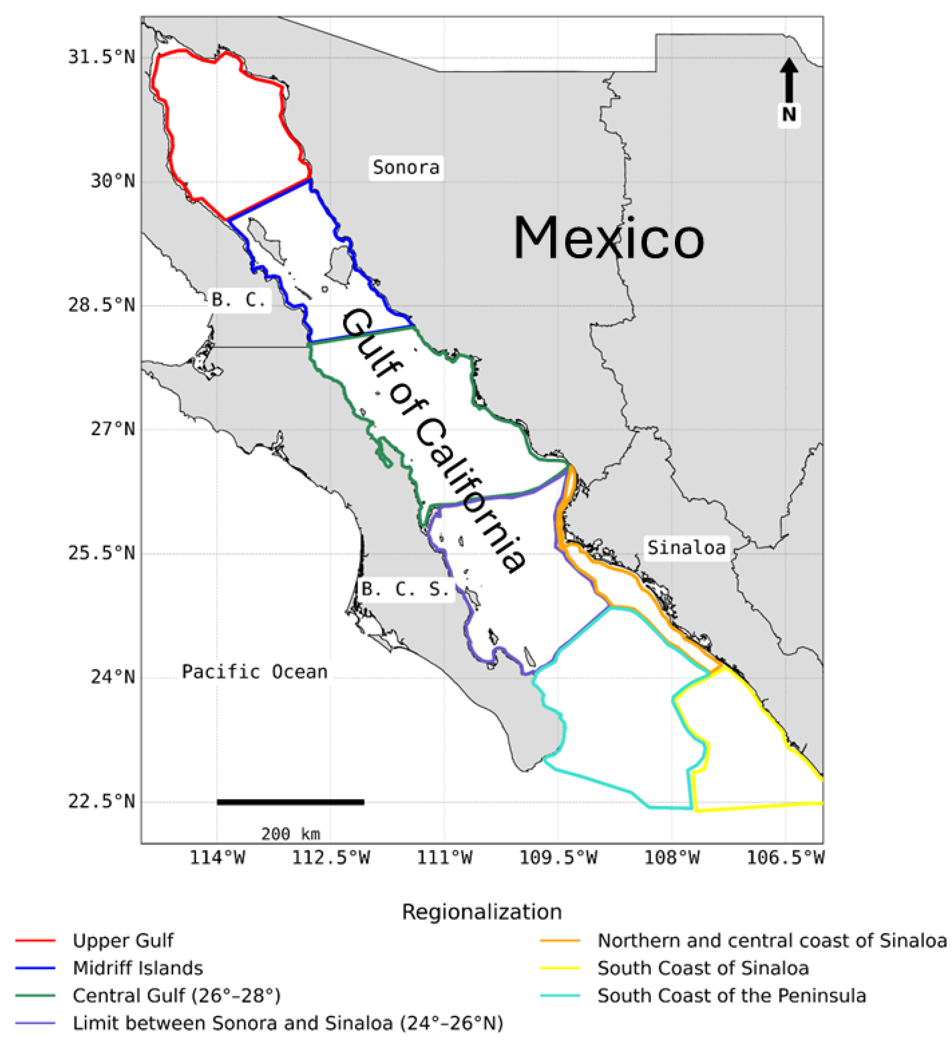
Figure 2.
Fast Fourier transform (FFT) for the Gulf of California sea surface temperature (SST) under the SSP1-2.6, SSP2-4.5, and SSP5-8.5 scenarios.
Figure 2.
Fast Fourier transform (FFT) for the Gulf of California sea surface temperature (SST) under the SSP1-2.6, SSP2-4.5, and SSP5-8.5 scenarios.
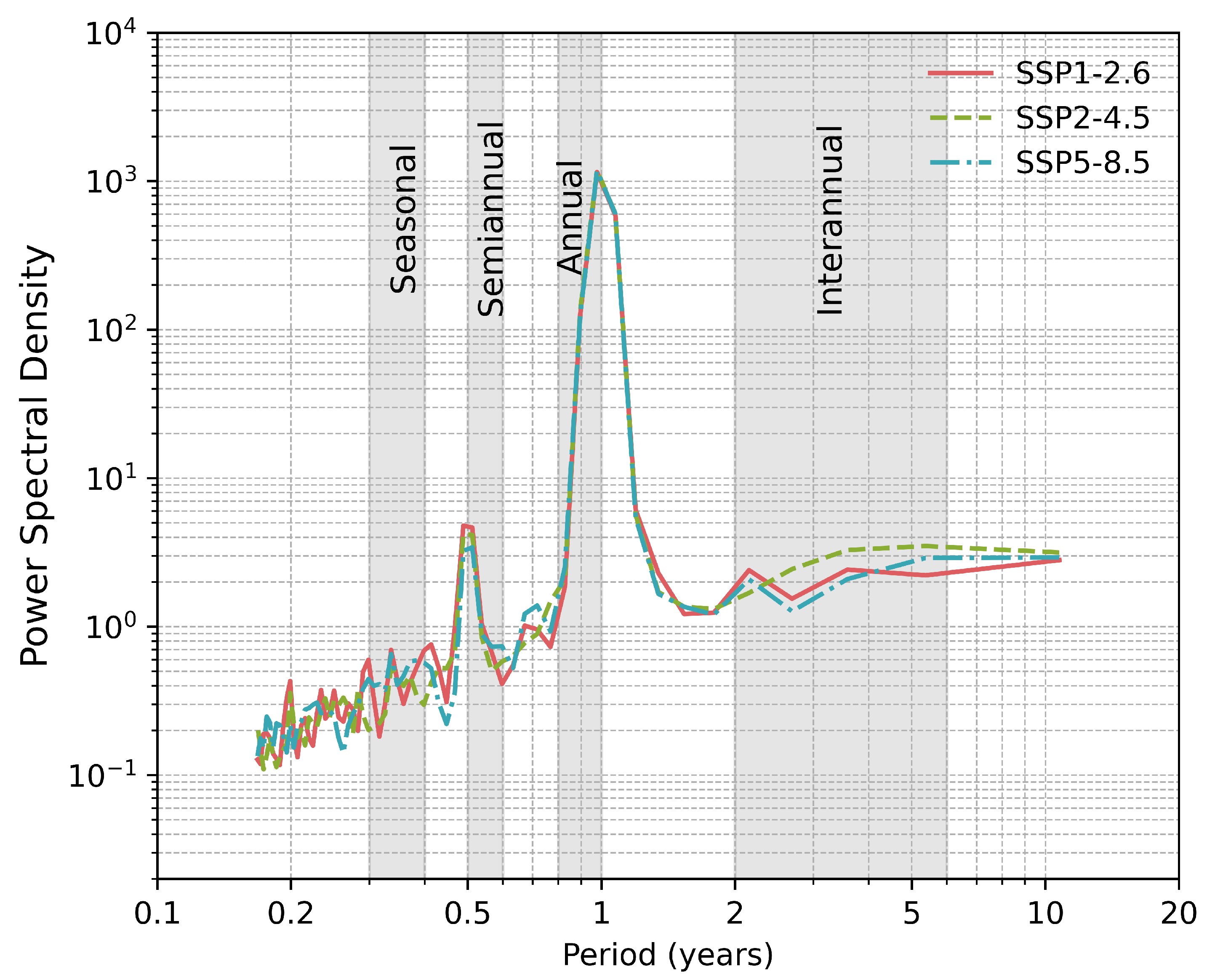
Figure 3.
Seasonal-Trend decomposition (STL) decomposition of the surface temperature of the Gulf of California under the SSP1-2.6, SSP2-4.5 and SSP5-8.5 scenarios.
Figure 3.
Seasonal-Trend decomposition (STL) decomposition of the surface temperature of the Gulf of California under the SSP1-2.6, SSP2-4.5 and SSP5-8.5 scenarios.
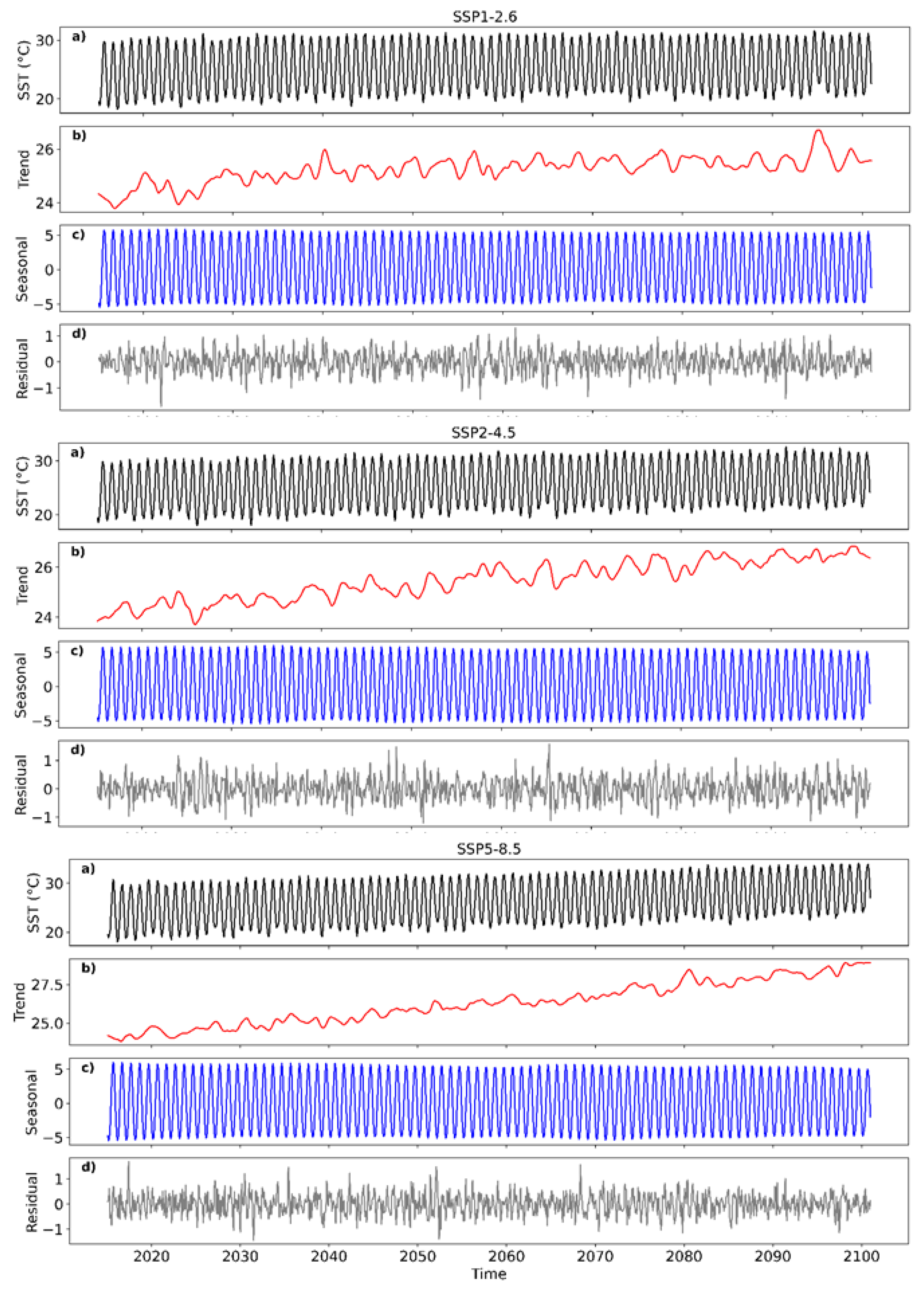
Figure 4.
Wavelet transform of sea surface temperature (SST) into the Gulf of California under the climate change scenarios SSP1-2.6 (upper panel), SSP2-4.5 (middle panel), and SSP5-8.5 (lower panel).
Figure 4.
Wavelet transform of sea surface temperature (SST) into the Gulf of California under the climate change scenarios SSP1-2.6 (upper panel), SSP2-4.5 (middle panel), and SSP5-8.5 (lower panel).
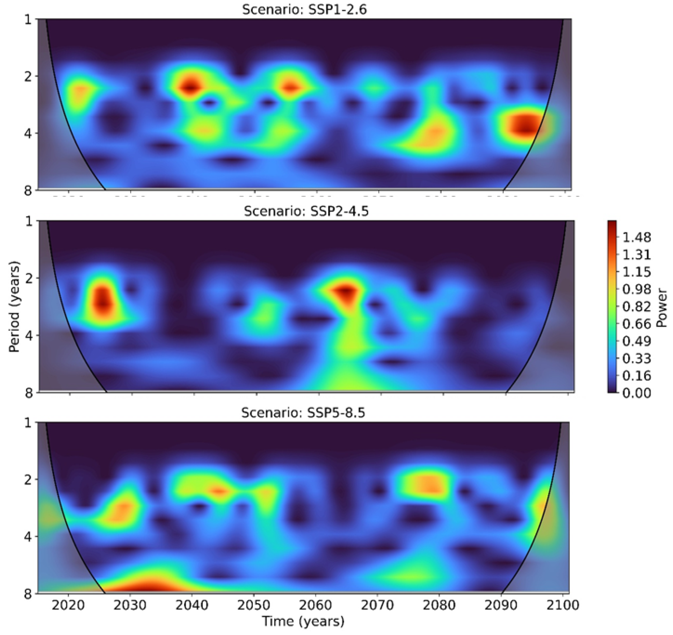
Figure 5.
Summer duration in days under each scenario (a), and extreme events (b).

Figure 6.
Rate change of the sea surface temperature under the scenarios SSP1-2.6 (a), SSP2-4.5 (b) and SSP5-8.5 (c).
Figure 6.
Rate change of the sea surface temperature under the scenarios SSP1-2.6 (a), SSP2-4.5 (b) and SSP5-8.5 (c).
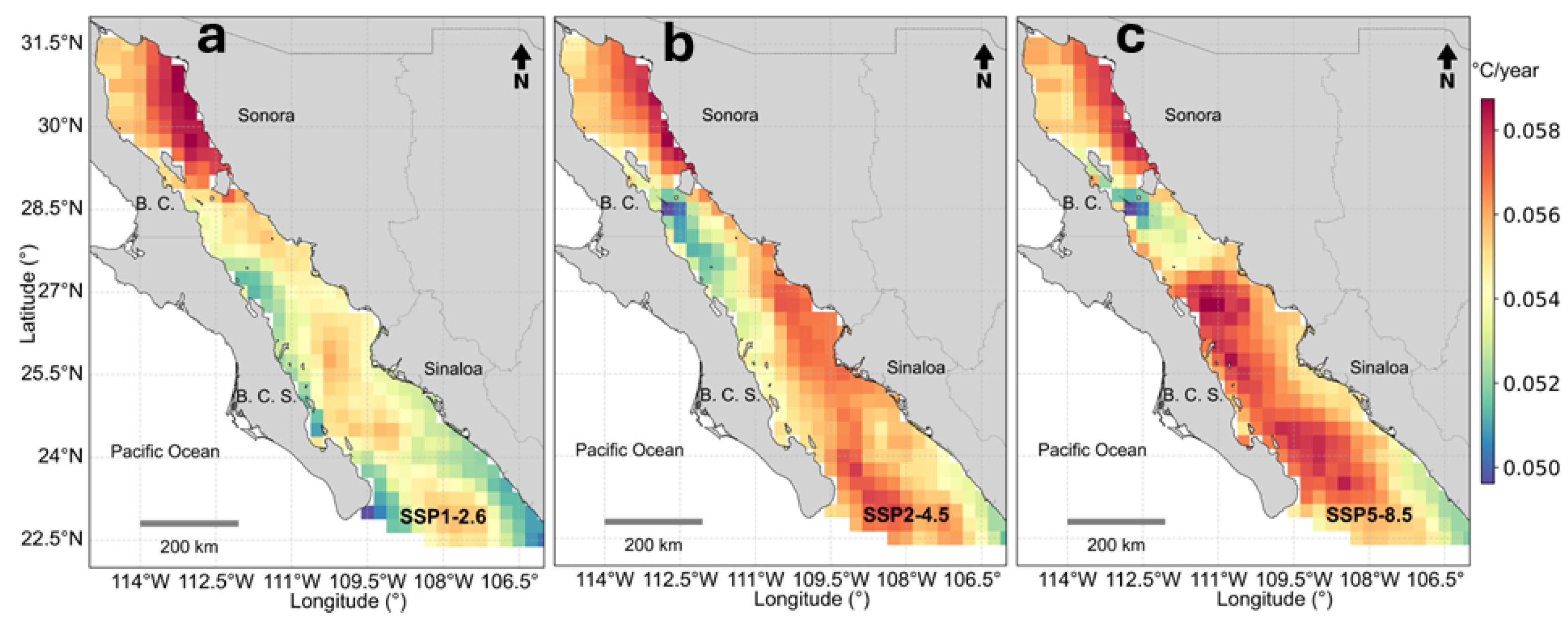
Figure 7.
Surface current speed (m s−1) from 2015 to 2100 under the SSP1-2.6, SSP2-4.5, SSP5-8.5 scenarios in the Upper Gulf, Central Gulf (26-28 °N) and Great Islands regions. *** denotes statistical significance of the slope.
Figure 7.
Surface current speed (m s−1) from 2015 to 2100 under the SSP1-2.6, SSP2-4.5, SSP5-8.5 scenarios in the Upper Gulf, Central Gulf (26-28 °N) and Great Islands regions. *** denotes statistical significance of the slope.
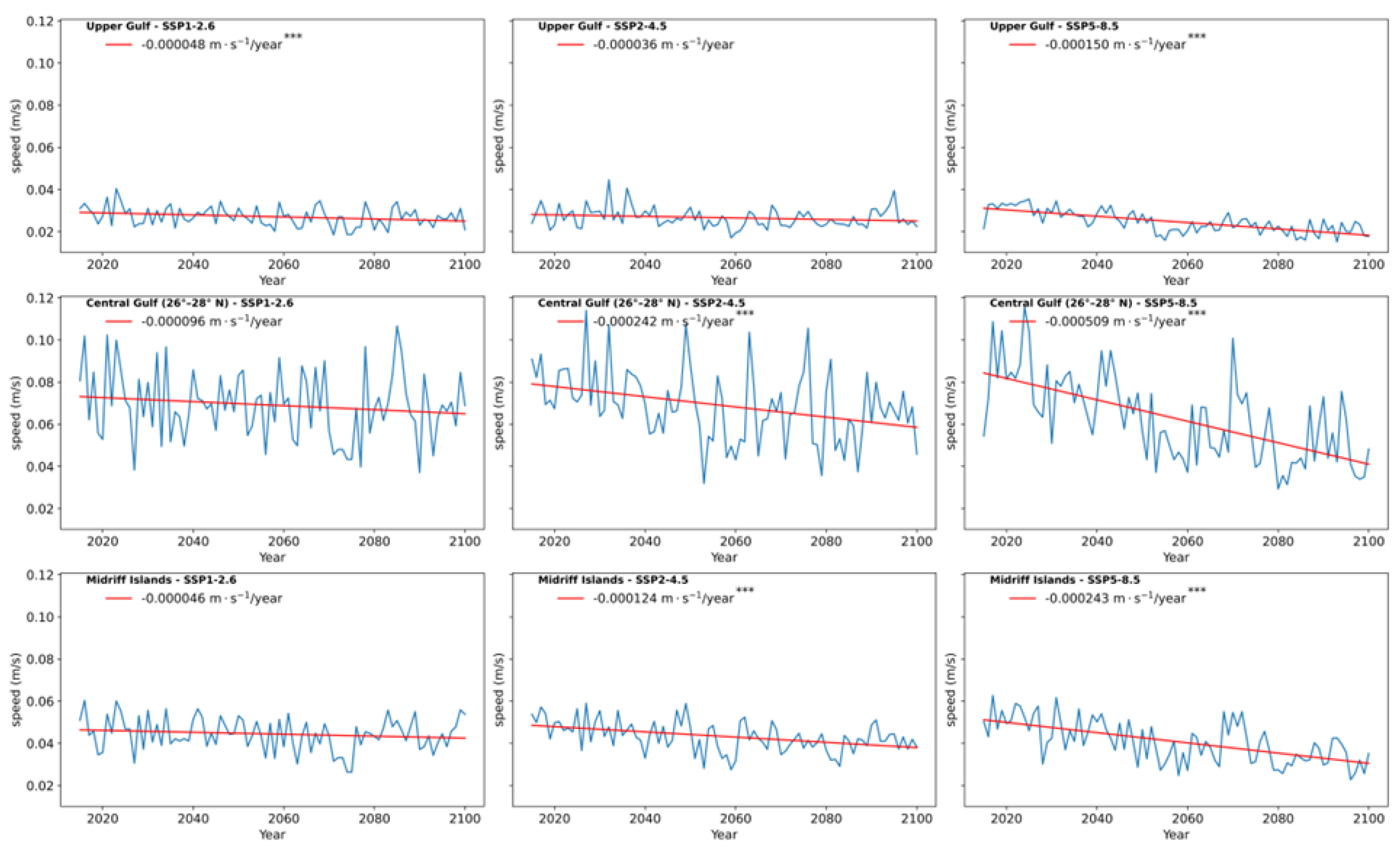
Figure 8.
Surface current speed (m s−1 from 2015 to 2100 under the SSP1-2.6, SSP2-4.5, SSP5-8.5 scenarios in the Limit between Sonora and Sinaloa (24-26 °N), South Coast of the Sinaloa, South Coast of the Peninsula and Northern and central Coast of Sinaloa.
Figure 8.
Surface current speed (m s−1 from 2015 to 2100 under the SSP1-2.6, SSP2-4.5, SSP5-8.5 scenarios in the Limit between Sonora and Sinaloa (24-26 °N), South Coast of the Sinaloa, South Coast of the Peninsula and Northern and central Coast of Sinaloa.
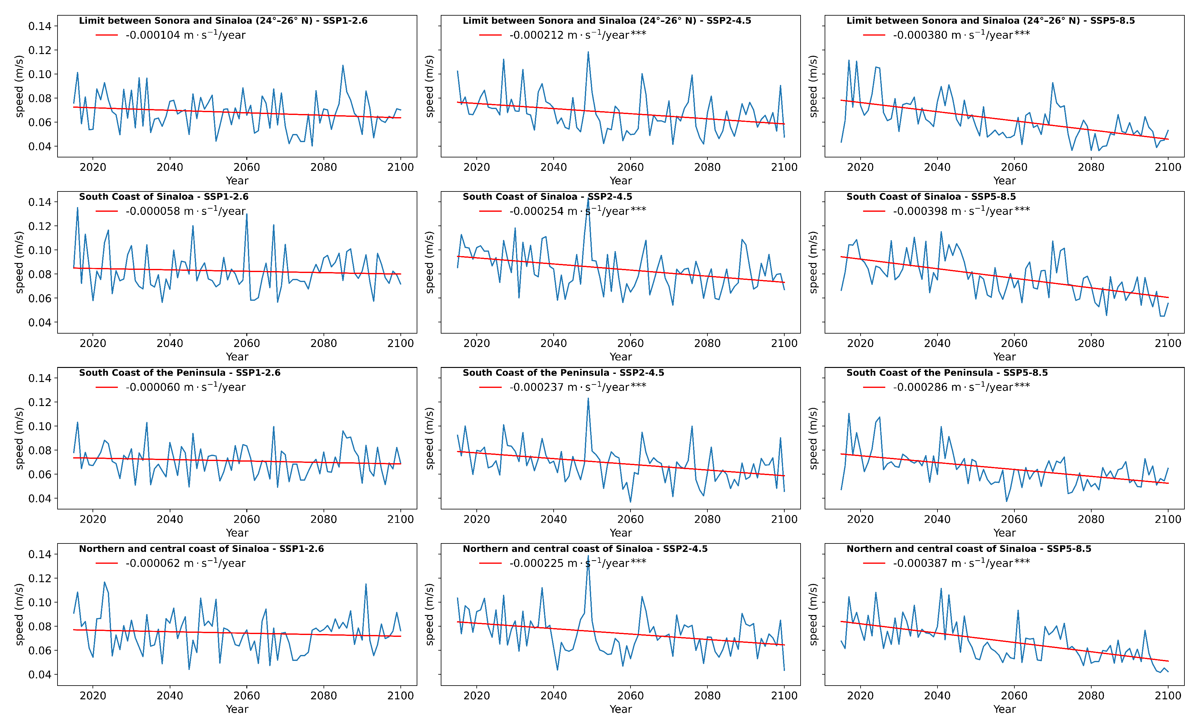
Figure 9.
Wind speed (m s−1) from 2015 to 2100 under the SSP1-2.6, SSP2-4.5, SSP5-8.5 scenarios in the Upper Gulf, Gulf Cen-ter (26-28° N) and Great Islands regions. *** denotes statistical significance of the slope.
Figure 9.
Wind speed (m s−1) from 2015 to 2100 under the SSP1-2.6, SSP2-4.5, SSP5-8.5 scenarios in the Upper Gulf, Gulf Cen-ter (26-28° N) and Great Islands regions. *** denotes statistical significance of the slope.
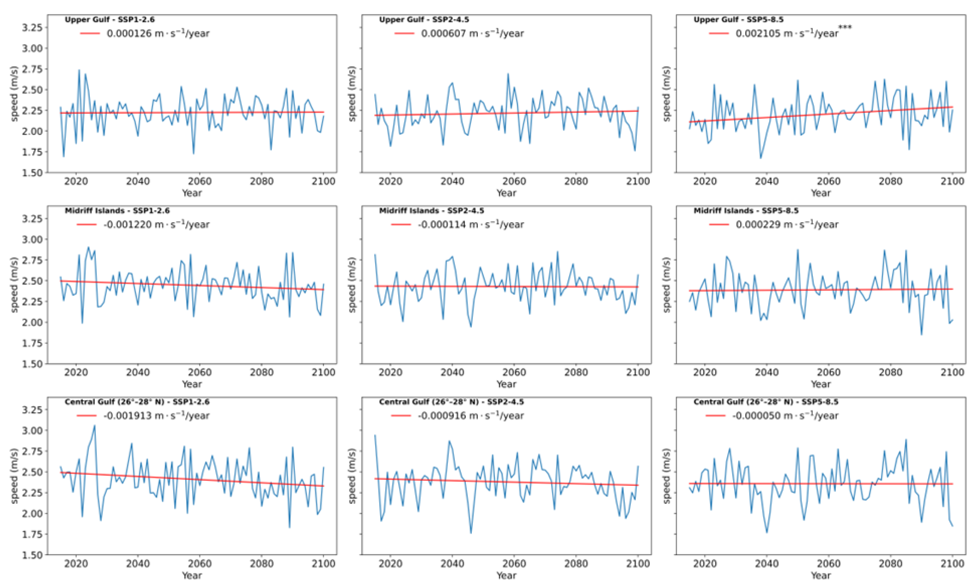
Figure 10.
Wind speed (m s−1) from 2015 to 2100 under the SSP1-2.6, SSP2-4.5, SSP5-8.5 scenarios in the Limit between Sonora and Sinaloa (24-26°N), Northern and central coast of Sinaloa, South Coast of the Peninsula and South Coast of Sina-loa regions. *** denotes statistical significance of the slope.
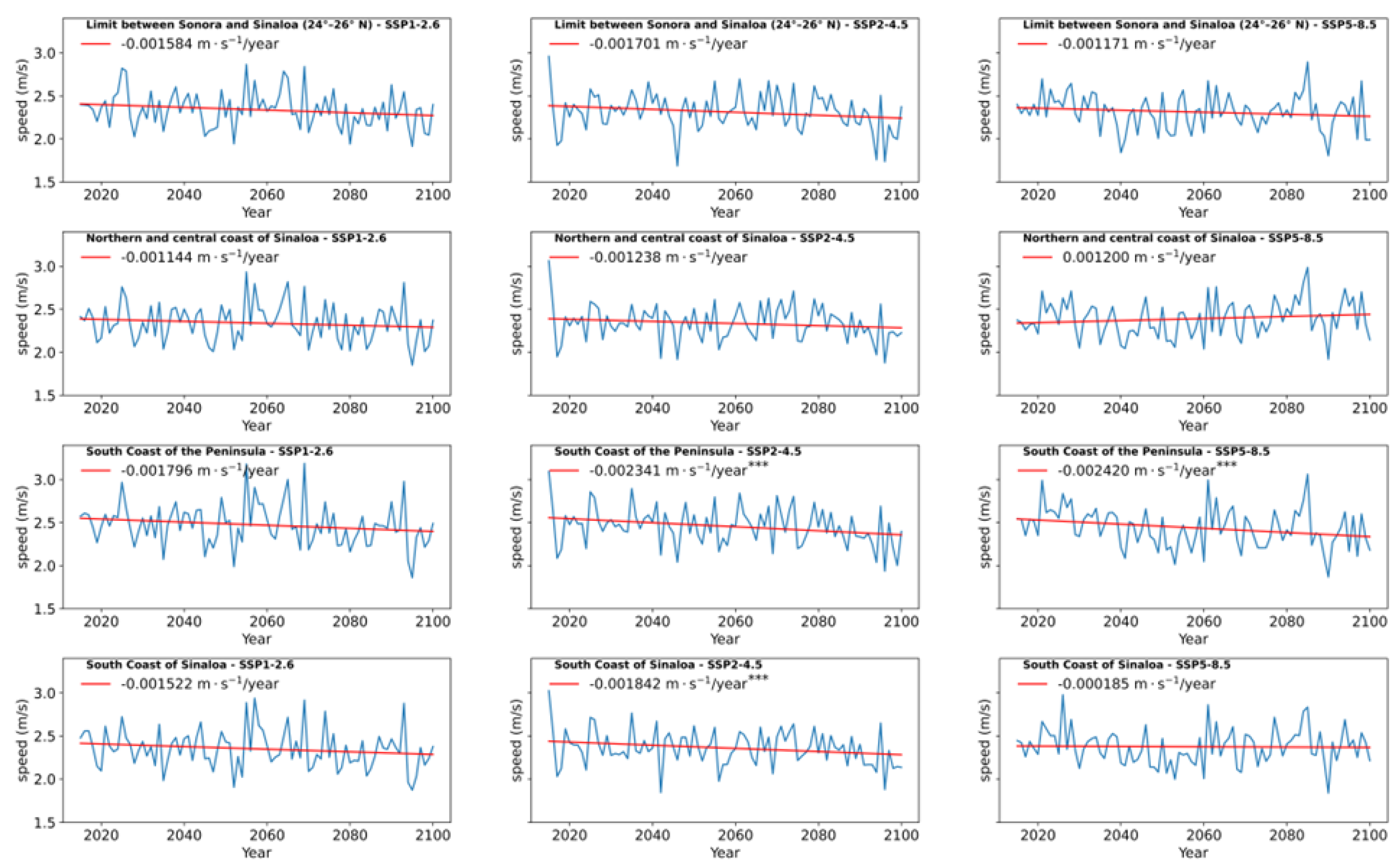
Figure 11.
Rate change of the wind speed under the scenarios SSP1-2.6 (a), SSP2-4.5 (b), and SSP5-8.5 (c).
Figure 11.
Rate change of the wind speed under the scenarios SSP1-2.6 (a), SSP2-4.5 (b), and SSP5-8.5 (c).
Disclaimer/Publisher’s Note: The statements, opinions and data contained in all publications are solely those of the individual author(s) and contributor(s) and not of MDPI and/or the editor(s). MDPI and/or the editor(s) disclaim responsibility for any injury to people or property resulting from any ideas, methods, instructions or products referred to in the content. |
© 2025 by the authors. Licensee MDPI, Basel, Switzerland. This article is an open access article distributed under the terms and conditions of the Creative Commons Attribution (CC BY) license (http://creativecommons.org/licenses/by/4.0/).
Copyright: This open access article is published under a Creative Commons CC BY 4.0 license, which permit the free download, distribution, and reuse, provided that the author and preprint are cited in any reuse.


