
Submitted:
01 December 2024
Posted:
02 December 2024
You are already at the latest version
Abstract
Over the past decade, several studies based on coupled ocean-atmosphere simulations have shown that the oceanic surface current feedback to the atmosphere (CFB) leads to a slow-down of the mean oceanic circulation and, overall, to the so-called eddy killing, i.e., a sink of kinetic energy from oceanic eddies to the atmosphere that damps the oceanic mesoscale activity by about 30%, with upscaling effects on large-scale currents. Despite significant improvements in the representation of western boundary currents and mesoscale eddies in numerical models, some discrepancies remain when comparing numerical simulations with satellite observations. These include a stronger wind and wind stress response to surface currents and a larger air-sea kinetic energy flux from the ocean to the atmosphere in numerical simulations. However, altimetric gridded products are known to largely underestimate mesoscale activity, and the satellite observations operate at different spatial and temporal resolutions and do not simultaneously measure surface currents and wind stress, leading to large uncertainties in air-sea mechanical energy flux estimates. ODYSEA is a new satellite mission project that aims to simultaneously monitor total surface currents and wind stress with a spatial sampling interval of 5 km and 90% daily global coverage. This study evaluates the potential of ODYSEA to measure surface winds, currents, energy fluxes, and ocean-atmosphere coupling coefficients. To this end, we generated synthetic ODYSEA data from a high-resolution coupled ocean-wave-atmosphere simulation of the Gulf Stream using ODYSIM, the Doppler scatterometer simulator for ODYSEA. Our results indicate that ODYSEA would significantly improve the monitoring of eddy kinetic energy, kinetic energy cascade, and air-sea kinetic energy flux in the Gulf Stream region. However, despite the improvement over the current measurements, the estimates of the coupling coefficients between surface currents and wind stress may still have large uncertainties due to the noise inherent in ODYSEA, but also due to measurement capabilities related to wind stress.
Keywords:
ODYSEA
; Doppler scatterometer
; surface currents
; wind stress
; eddy kinetic energy
; horizontal energy fluxes
; wind work
; coupling coefficients
1. Introduction
In the last couple of decades, thanks to advances in numerical modeling and satellite observations, mesoscale air-sea interactions have received a growing interest from the scientific community. In particular, the Current FeedBack to the atmosphere (CFB; [1,2,3,4,5]), which is essentially the influence of surface currents on the overlying atmosphere, has been shown to be a missing piece in ocean modeling. CFB has been shown to slow down the mean oceanic circulation [6,7] and, overall, to induce the so-called eddy killing effect, i.e., a sink of kinetic energy from oceanic eddies to the atmosphere that damps the oceanic mesoscale activity by about 30% [5,8,9,10]. The sink of kinetic energy caused by CFB arises from the interaction between surface currents, winds, and wind stress: a positive (negative) current anomaly induces a negative (positive) wind stress anomaly and, hence, a positive (negative) wind anomaly [5]. The damping of the oceanic mesoscale activity further leads to a weakening of the eddy-mean flow interaction (the inverse cascade of kinetic energy), stabilizing and improving the representation of emblematic western boundary currents such as the Gulf Stream, the Agulhas Current, and the Loop Current [7,11,12,13,14,15]. Furthermore, the current feedback promotes the occurrence of mesoscale eddies with more realistic properties (e.g., thermohaline characteristics, energy levels, and lifetime) and trajectories by modifying their detachment location, periodicity, and interactions with the atmosphere [5,15].
As a measure of the eddy killing effect, the wind work has been broadly used to investigate the extent to which CFB modulates the intensity of wind-driven currents, i.e., Ekman currents, near-inertial oscillations, and internal gravity waves, as well as (sub)mesoscale and large-scale currents [5,9,15,16,17,18,19,20]. CFB efficiency can also be characterized by means of the coupling coefficient , which is defined as the slope of the linear regression between mesoscale surface current vorticity and wind stress curl: The more negative the , the more efficient the eddy killing.
However, despite significant improvements in ocean dynamics in numerical models, discrepancies remain when coupled numerical simulations are compared with satellite observations. Coupled ocean-atmosphere simulations exhibit a stronger wind stress response to CFB, a larger eddy wind work, and, consistently, a more negative coupling coefficient compared to those estimated from the combination of altimeter (AVISO product, [21]) and scatterometer products [22] (see [7,8,23]). While no doubt some of these discrepancies are due to model bias, the current satellite products have large systematic errors and important sampling differences. In particular, the AVISO product largely underestimates the mesoscale levels of energy and can only resolve mesoscale eddies with a diameter larger than 100 km [24,25,26,27]. In addition, satellite observations operate at different spatial and temporal resolutions and do not simultaneously measure surface currents and wind stress, which is critical for accurate quantification of kinetic energy flux between the ocean and the atmosphere (the windwork) and the coupling coefficient [8,28]. Finally, because scatterometers provide winds relative to oceanic currents, they cannot adequately characterize the CFB wind response.
The Ocean Dynamics and Sea Exchanges with the Atmosphere (ODYSEA) satellite project, which includes a Doppler scatterometer, would allow us to simultaneously measure total surface currents and winds with a spatial resolution of 5 km, temporal resolution of 12 hours, and global coverage within 1-2 days. Measurement errors follow Gaussian distributions with standard deviations of 50 cm for currents in low wind conditions and 1 m for winds [28,29,30]. A previous study of [28] analyzed the ODYSEA capability of estimating wind work and its sensitivity to measurement uncertainties. The authors use a measurement simulator fed by results from a 4 km ocean-atmosphere coupled simulation to show that ODYSEA sampling would properly represent the wind work, even if surface current errors reach 1 m .
This study aims to go one step further by assessing how well ODYSEA could measure surface winds, currents, energy fluxes, and ocean-atmosphere coupling coefficients. To this end, we generate synthetic ODYSEA data from a coupled ocean-surface-waves-atmosphere high-resolution numerical simulation of the Gulf Stream and using the Doppler scatterometer simulator ODYSIM (https://github.com/awineteer/odysea-science-simulator). Our study focuses on the Gulf Stream region, which is characterized by strong and large (sub)mesoscale currents but also by the occurrence of large surface gravity waves (Figure 1).
The paper is organized as follows. Models, ODYSEA simulator, and datasets used in this work are described in Section 2. Section 3 demonstrates the capabilities of ODYSEA to reproduce the ocean surface kinetic energy and wind stress, as well as kinetic energy cascades, air-sea energy fluxes related to wind work, and ocean-atmosphere coupling coefficients. This section also analyzes the consequences of measurement uncertainties, e.g., sub-sampling and noise, and proposes strategies for dealing with them. Finally, the results are discussed in Section 4.
2. Methods and Data
2.1. ODYSIM
ODYSIM is a Doppler scatterometer simulator designed to explore the capabilities of ODYSEA. It generates synthetic ODYSEA data from numerical simulations to assess the measurement of surface currents and winds [28,30]. The simulator is configured with the following specifications: a satellite with a 5.0 × 0.35 m antenna, 400 W transmit power, a 590 km sun-synchronous polar orbit with a 4-day repeat cycle, and an incidence angle of 56°. This configuration allows a wide measurement swath of about 1700 km with a daily global coverage of around 90% and a spatial resolution of 5 km for surface currents and winds [28,29,30].
ODYSIM allows assessing the potential consequences of inherent uncertainties in the measurements because it includes a parametrization of random errors or noise, which largely depend on the wind speed and the look geometry [30,31]. The commonly referenced performance baseline noise for ODYSEA is stated as 50 cm for surface currents and 1 m for surface winds for a spatial sampling interval of 5 km [29]. However, [30] demonstrate that noise associated with surface current measurements can be significantly higher at the center and edges of the swath, while it diminishes over the "sweet spots," which are the regions between the center and the edges.
In this study, ODYSIM generates synthetic ODYSEA measurements by extracting surface currents and wind stress data from a high spatial resolution coupled ocean-atmosphere-wave simulations performed over the Gulf Stream region. The details of the configuration are provided below.
2.2. Coupled Ocean-Surface Waves-Atmosphere Numerical Simulation
The coupled ocean-atmosphere-wave system uses the Coastal and Regional Ocean Community (CROCO) version of the Ocean Modeling System (ROMS) model [32,33] to reproduce the ocean dynamics at a spatial resolution of 1/42° (∼2.2 km), the Weather Research and Forecast (WRF) model [34] to reproduce the atmosphere dynamics with a spatial resolution of 1/15° (∼6 km), and the WaveWatch III (WW3) surface gravity wave models to simulate sea state with a spatial resolution of ∼6 km. The domains for CROCO, WRF, and WW3 are illustrated in Figure 2a. The numerical models and configurations are similar to the ones employed in [35,36], and the following model descriptions are derived from those references with minor modifications. Briefly, the simulations are in good agreement with observations, as shown by [18,35,36] and reproduce a stable path of the Gulf Stream with an intense mesoscale activity around, a realistic atmospheric low-level circulation and heat fluxes, and a fair representation of the surface gravity waves.
2.2.1. The CROCO Configuration
The CROCO model is a terrain-following, free-surface Boussinesq model that uses a split-explicit time-stepping scheme. While it is available in both hydrostatic and non-hydrostatic versions, we used the hydrostatic version in this study.
A fifth-order upstream biased momentum advection is used [37,38], which reduces the numerical dispersion and diffusion and allow to achieve an effective resolution of about 10 km (about 5 times the horizontal resolution). For horizontal tracer transport, the model employs a rotated split third-order upstream scheme for discretization. Notably, the diffusive component of this scheme is rotated along isopycnal surfaces, a method aimed at minimizing excessive diapycnal mixing, as suggested by [39,40], and [41]. To represent turbulent diffusion processes at the surface, bottom, and interior of the ocean, the K-Profile Parameterization (KPP; [41]) is used.
As depicted in Figure 2, the CROCO model is implemented over the North West Atlantic Ocean with a horizontal spatial sampling interval of (∼ 2.2 km). It extends from 22.5°N to 48.84°N and from 36°W to 82°W. The full configuration is described in [35] as the “TD” simulation, i.e., a simulation that is forced at its lateral boundary by the 1/12°daily mean Mercator Glorys12V1 product [42], and by barotropic tides (height and currents) from the global tidal model TPXOv.7 [43]. Bottom drag is quadratic and parameterized through a logarithmic law of the wall with a roughness length of m. The coupled simulation runs for one year, starting on January 1st, 2005, after a spin-up of 5 years (see [18] for more details).
2.2.2. The Weather Research and Forecast Model Configuration
WRF 4.2 [34] is implemented over a slightly larger domain to avoid issues related to the sponge layer of WRF. It has a horizontal spatial sampling interval of approximately 6.2 km [36] and used 50 hybrid hybrid-levels with a model top pressure set at 1000 Pa and a first level at 10 meters over the ocean. The model is initialized and forced at its lateral boundary by the ERA5 dataset [44].
We used the following set of parameterizations: the KIAPS SAS (KSAS) convective scheme [45,46], the WRF Single-moment 6-class (WSM6) microphysics scheme with droplet concentration inclusion [47,48], the Dudhia shortwave radiation scheme [49], the Rapid Radiative Transfer Model Longwave Radiation Scheme [50], the Yonsei University (YSU) Planetary Boundary Layer Scheme [51], the Revised MM5 Surface Layer Scheme [52], and the Noah Land Surface Model [53]. The current feedback parameterization is implemented in both the surface layer and planetary boundary layer schemes, following the approach of [54].
2.2.3. The WaveWatch III Model Configuration
WW3 solves the random phase spectral action density balance equation for specific wavenumber-direction spectra, encompassing various physical processes. These include wind-wave interactions, nonlinear wave-wave interactions, wave-bottom interactions, depth-induced breaking, dissipation, and shoreline reflection, all of which are parameterized within the model. To address numerical artifacts arising from discrete directions of wave propagation, the third-order Ultimate Quickest scheme by [55], augmented with the Garden Sprinkler correction, is employed. Nonlinear wave-wave interactions are accounted for using the Discrete Interaction Approximation (DIA) method proposed by [56]. The wind-wave interaction source term introduced by [57] is integrated into the model, featuring a parameterization based on saturation-based dissipation to mitigate unrealistically large drag coefficients observed under high wind conditions. Furthermore, depth-induced wave breaking, following the formulation by [58], and bottom friction source terms as outlined by [59] are incorporated.
The grid used in the WW3 model covers the same geographic region and has the same spatial resolution as the Weather Research and Forecasting (WRF) model. Specifically, the spectral discretization used in WW3 consists of 24 directions (at 15° intervals) and 32 frequency bins. To establish lateral boundary conditions for the coupled simulations, a stand-alone WW3 simulation is performed over the entire Atlantic region for the period 2004 to 2006. This stand-alone simulation uses the same spectral discretization and a spatial resolution of 0.2°. The wind forcing data used in this stand-alone simulation is obtained from the Climate Forecast System Reanalysis (CFSR) dataset [60]. The derived spectra from this stand-alone WW3 run are then imposed hourly at the boundaries of WW3 in the coupled simulations.
2.2.4. Coupling Strategy
The coupling strategy is illustrated in Figure 2. The OASIS coupler [61] is used at the interface of the models to perform the exchanges of the different fields. The following fields are exchanged hourly between the models:
- WRF sends to CROCO momentum (surface stress), heat, and freshwater flux and receives from CROCO the sea surface temperature and currents.
- WRF sends to WW3 the wind and receives the Charnock parameter from WW3.
- CROCO gives the sea surface height and the surface currents to WW3 and receives the net wave-supported stress and wave-to-ocean momentum flux, as well as the significant wave height, mean wave period, and mean wave direction used to compute the Stokes Drift.
2.3. ODYSEA Datasets
Two main datasets are built from ODYSIM results, corresponding to along-track and gridded formats. Besides, additional datasets are generated by adding parametric measurement noise to the primary datasets and by applying spatial filters to reduce this noise. A summary of the properties of the generated datasets is shown in Table 1. To differentiate between the datasets generated from the ODYSIM simulator and the outputs of the coupled simulation, we adopted the following naming convention:
- The first three letters are "ODS" to denote that the dataset is generated by ODYSIM.
- Following "ODS", the dataset level is indicated: "L2" and "L3". "L2" represents the ODYSEA along-track data mapped onto a standardized grid with a resolution of 5 km. "L3" indicates a gridded dataset obtained by applying a running mean to the L2 products.
- The specific running mean applied is then specified: "1.5-day" or "3-day".
- The letter "N" indicates the presence of noise introduced into the dataset. Measurement noise depends on instrument parameters, look direction, and the strength of the return signal. The signal strength is proportional to the radar cross section, which depends on wind speed and direction through an empirically derived wind geophysical model function [30,31].
- To mitigate measurement noise, spatial smoothing is implemented using a window of either 15 km or 25 km. In such instances, the use of a spatial filter is denoted by the prefix "F," followed by the length of the spatial filter (15 or 25 km).
In the L2 products, following [28,30], the center and edges of the swat are removed to eliminate the regions with large uncertainties. In addition, surface currents where winds are weaker than 3 m are removed to ensure averaged errors of about 50 cm (Figure 3b). This excludes about 20% of the data (Figure 3a) but improves the representation of surface currents. Analyzing L2 datasets would allow us to quantify the uncertainties related to satellite sub-sampling. L3 datasets are necessary to compute horizontal energy fluxes and coupling coefficients between the sea surface currents and the atmosphere (See Section 3.3 and Section 3.4). Therefore, comparisons from "L2" to "L3" datasets will help us assess the consequences of temporal filters on the computation of these parameters. Comparing "N" and "L" datasets will enable us to identify how parametric noise affects data values in terms of statistical properties. Finally, a comparison between "N" and "F" datasets will allow us to analyze the effectiveness of spatial filters in reducing the impact of noise in ODYSEA measurements.
An example of the surface currents and wind stress are depicted in Figure 4. At first glance, both and are able to reproduce the mesoscale activity, mainly differing in the occurrence of spatial gaps related to the exclusion of the data at the center and edges of the swat in (Figure 4a,c,e). Regarding wind stress, it is evident that longer averaged periods promote an important smoothing over the fields (Figure 4b,d,f). This is associated with the propagation of fast atmosphere features, i.e., storms, that can not be properly sampled by the satellite [28].
2.4. Satellite “Like” Products
An important part of this work is to compare the future performance of ODYSEA with contemporaneous satellite missions. Therefore, we also generated datasets that mimic daily estimations of surface currents from AVISO [21,62] and wind stress from QuikSCAT [63] by filtering the reference simulation in space and time. The AVISOlike dataset is generated by applying a 7-day running window and an 85 km diameter spatial filter to the sea level height [13]. Subsequently, surface currents are computed through the application of the geostrophic balance, thus excluding ageostrophic motions as Ekman and cyclogeostrophic currents. The QuikSCATlike dataset is derived by applying a 1-day running mean filter and a 100 km diameter spatial filter to the wind stress components [8,28,64]. We also define the Obslike dataset as a combination of the AVISOlike and QuikSCATlike datasets. A summary of the filters applied to the reference experiment is shown in Table 2.
2.5. Kinetic Energy Fluxes
ODYSEA will be able to concurrently measure surface currents and wind stress. This dual functionality enables us to compute not only horizontal energy fluxes of surface currents but also the flux of kinetic energy between the ocean and the atmosphere, i.e., the wind work. In this study, both energy fluxes are computed using a coarse-graining decomposition [65].
The coarse-graining method allows estimating the energy flux related to a certain spatial scale [18,35,65,66,67,68,69]. The method is based on the separation between large and small scales around chosen scales, L. The signal is separated by applying a two–dimensional running mean with diameter L to a field . This filter results from applying a convolution with a top–hat kernel
Here, is the circular normalization area of diameter L, and is the radial position vector [68].
Following [68], applying the convolution to the equation of motion results in a term that allows us to estimate the horizontal energy flux () for a certain scale L:
where u and v represent the zonal and meridional components of surface currents, respectively. As mentioned by [65], this term is similar to barotropic instability, which relates to energy transfer between mean and eddy kinetic energy. With the coarse-grained method, positive values of imply an energy flux to smaller scales (forward cascade), whereas negative values imply and energy flux to larger scales (inverse cascade).
Likewise, eddy wind work () is derived from coarse–grained filtered fields:
where and correspond to the zonal and meridional components of wind stress. Positive values of indicate that the atmosphere is injecting energy into the ocean at the scale L, whereas negative values indicate energy fluxes in the opposing direction [69].
2.6. Coupling Coefficient
The coupling coefficient allows us to assess the efficiency of the eddy killing process. Following in [5,8], is computed as the slope of a linear regression between surface ocean currents vorticity anomalies and surface stress curl anomalies. To isolate the mesoscale signal and to remove the atmospheric synoptic variability, anomalies result from a 31-day low pass filter and a 275-km high pass filter. It is worth mentioning that regions with quasi-stationary weather conditions, e.g., atmospheric blocking events [70,71], require long averaging times to isolate the mesoscale signal. In order to deal with track overlaps and uncertainties in ODYSEA gridded datasets, is computed from the noisy level 2 datasets N and N, followed by the application of a 25-km low pass filter.
3. Results
The purpose of this section is to assess the extent to which ODYSEA would capture the surface currents and the associated oceanic kinetic energy, the wind stress, the oceanic cascade of kinetic energy, the exchange of kinetic energy between the (sub)mesoscale eddy and the atmosphere, and the coupling coefficient . We examine the ability of ODYSEA to capture these fields and aim to understand the impact of uncertainties on their estimation.
3.1. Kinetic Energy of Surface Currents
The surface mean and eddy kinetic energy (MKE and EKE) from the reference simulation, as well as for the ODYSEA and observations-like datasets are estimated as:
where and are the surface currents. The ¯ represents the annual mean and the ′ denotes the deviations from the mean. Figure 5 shows the main analysis. The MKE estimated from the reference experiment shows a realistic representation of the Gulf Stream dynamics. The Gulf Stream flows northward along the entire Florida coast up to Cape Hatteras (35°N), where it begins to separate from the coast, veering eastward (Figure 5a). Post-separation, large eddies detach from the Gulf Stream and propagate westward, leading to an intense mean mesoscale activity around the Gulf Stream path (up to 0.2 ; Figure 5b).
The AVISOlike and ODYSEA datasets can reproduce the main spatial patterns of MKE and EKE (Figure 5a-h). However, while the MKE appears to be similar in all the datasets, there are notable discrepancies in the intensity of the EKE estimates. To quantitatively assess these differences over the Gulf Stream, EKE estimates are spatially averaged over the polygon delineated in Figure 5b and visually presented in Figure 5i.
Not surprisingly, and consistent with the literature, the results reveal that AVISOlike tends to underestimate the EKE by approximately 54%. In contrast, ODSL2, which does not consider the measurement error, shows a minimal underestimation of the EKE (about 1.5%), exhibiting that the sampling capabilities per se of ODYSEA allow an adequate estimation of the EKE over the Gulf Stream. It is worth noting that from ODSL2 to ODSL2N, measurement noise spuriously increases the EKE by about 22% (ODSL2N dataset in Figure 5i). In , however, the spurious EKE is largely removed by applying a 15 km diameter low-pass filter to the surface currents (ODSL2N to in Figure 5i).
Time averages used to perform ODSL3 datasets have large consequences on the estimation of EKE. On the one hand, the and datasets underestimate the EKE by about 15% and 20%, respectively. However, the gridded products of surface currents and wind stress are essential for computing, for example, air-sea coupling coefficients or coarse-grained energy fluxes. On the other hand, time averages help to reduce uncertainties related to noise in the EKE calculation (Figure 5i). The time-averaged noise datasets, N and N, have increased EKE estimates from the noise-free datasets by only 16% and 15%, respectively, while EKE estimates from ODSL2 to ODSL2N increase by 22%. Finally, the effect of noise on EKE estimation is mitigated by applying a 25-km low-pass spatial filter to N and . Despite the underestimation of the EKE at various degrees depending on the considered dataset, ODYSEA should improve its representation compared to current altimeter estimations.
While spatial filters help to reduce measurement noise, they also have the disadvantage of reducing the fine-scale variability of ocean currents. To better characterize which scales are effectively measured by ODYSEA, a two-dimensional co-spectral analysis was performed on the KE to evaluate the performance of the ODYSEA datasets (Figure 6). The analysis reveals that all ODYSEA datasets accurately capture the KE at the large and large mesoscale (wavelengths larger than 100 km) and exhibit energy decay rates around (Figure 6). Nevertheless, the sampling capabilities of ODYSEA can lead to a 20% underestimation of energy across wavelengths around 50 km ( and in Figure 6a).
In N and N, measurement noise leads to a significant overestimation of kinetic energy levels at wavelengths less than 80 km (Figure 6b). Consistent with previous analyses, the application of 15- and 25-km low-pass spatial filters (Figure 6c,d) effectively attenuates these spurious kinetic energy levels. While the 15-km spatial filter reduces noise effects, particularly at scales smaller than 50 km wavelengths, the energy estimates for and still show an overestimation compared to the noise-free data sets ( and ) around 20 km wavelengths. In contrast, the 25 km spatial filter, though reducing the effective resolution of ODYSEA to about 35 km, yields more accurate energy level estimates at smaller wavelengths, with only about 7% underestimation observed at wavelengths around 50 km. Despite the consequences of spatial and temporal filters applied to ODYSEA datasets, these filters largely improve the representation of the kinetic energy in comparison with the AVISOlike dataset, which underestimates energy estimations by about 75-85% at wavelengths between 100 and 50 km and fails to detect smaller scale features.
3.2. Surface Wind Stress
The wind stress time mean and standard deviation for the reference simulation, as well as for the QuikSCAT-like and ODYSEA data sets, are shown in Figure 7. In the reference simulation, mean wind stress values exceed 0.05 N above 35°N and below 25°N, while weaker values (less than 0.025 N ) are observed around 30°N (Figure 7a). Regarding the wind stress variability, it shows a standard deviation greater than 0.2 N above 33°N, with more intense values (greater than 0.3 N ) throughout the Gulf Stream (gray contour in Figure 7b).
Mean wind stress conditions are accurately reproduced by QuikSCATlike and ODYSEA datasets (Figure 7a,c,e,g). While these datasets effectively capture the spatial distribution of strong wind stress anomalies (larger than 0.2 N ), notable differences emerge when spatially averaging the standard deviation over the polygon depicted in Figure 7a. QuikSCATlike tends to underestimate wind stress variability by approximately 17% over the Gulf Stream region (Figure 7i). In contrast, the sampling capabilities of ODYSEA allow reliable estimations of the wind stress variability across the Gulf Stream, albeit with a slight underestimation of about 5% in ODSL2 with respect to the reference simulation (Figure 7i).
Moreover, because ODYSEA allows wind speed errors below 1 m , the standard deviation increases by only 5% when considering the parameterized noise, and is reduced to 3% when applying a 15 km low-pass spatial filter (ODSL2, ODSL2NF, and in Figure 7i).
Conversely, the and datasets significantly underestimate the wind stress standard deviation compared to ODSL2 (30 and 40%, respectively). This significant underestimation is primarily due to the time averages used to construct gridded products, which limit the ability to capture the transient variability of atmospheric dynamics, such as storms, which evolve faster than ocean dynamics [28]. With respect to measurement noise in wind stress, it does not appear to play a critical role in masking atmospheric dynamics.
3.3. Cascade of Kinetic Energy
Following [35], Figure 8 estimates the surface cascade of kinetic energy for each dataset using a coarse-grained approach [65]. Figure 8a shows the spatially averaged kinetic energy flux over the polygon depicted in Figure 8b, while Figure 8b-i exhibit the spatial distribution of horizontal energy fluxes at small (20 km) and large (150 km) scales.
In agreement with [35], the reference simulation shows a predominant forward cascade energy fluxes on scales smaller than 50 km over the Gulf Stream region (Figure 9a), with a peak around 10 km scales. The spatial distribution of horizontal energy fluxes at the small scale (20 km; Figure 9b) shows positive energy fluxes stronger than 100 mW km east of the Gulf Stream separation. Besides, the figure exhibits a less intense forward cascade of about 50 mW / km west of the Gulf Stream separation. The forward cascade of energy is driven by nonlinear interactions between balanced and unbalanced currents [18], which align with the large-scale meandering patterns of positive energy fluxes all over the Gulf Stream (gray contours in Figure 9a). However, as pointed out by [35], forward cascade energy fluxes are also influenced by the interaction of internal tides and unbalanced motions. On scales larger than 50 km, as expected, there is a strong inverse cascade of energy with a peak at about 160 km. Unlike the forward cascade, the inverse cascade is driven by balanced (mostly geostrophic) currents [13]. The spatial distribution of horizontal energy fluxes at the large scale (150 km; Figure 8c), in spite of being dominated by the inverse cascade, reveals alternating forward and inverse cascade energy fluxes all along the Gulf Stream (gray contour in Figure 8c). It is worth mentioning that these results (Figure 9c) appear noisy with respect to [35] because the energy cascades are estimated for only 1 year instead of 5 years in [35].
Regarding the AVISOlike product, it does not show any significant forward energy cascade (Figure 9a). This can be explained by the inherent limitations of AVISO. On the one hand, AVISO is heavily smoothed [26] and, therefore, cannot resolve fine-scale eddies. On the other hand, AVISO lacks the ageostrophic currents that are essential to capture the forward cascade of energy in the Gulf Stream [18,35]. Consistent with previous studies, e.g., [13,25], the inverse cascade energy fluxes in AVISOlike are largely underestimated with respect to the reference simulation and shifted to larger scales, with the most intense values around 400 km. A comparison of the spatial distribution of horizontal energy fluxes at the 150 km scale provides valuable insights into understanding these differences (Figure 9c,i). The comparison reveals that the weak inverse cascade energy fluxes in AVISOlike (Figure 9a) result from weaker and alternating positive-negative energy fluxes (less than 50 mW / km), which lack the predominant negative energy fluxes seen in the reference simulation (Figure 9b).
For ODYSEA, as explained in Section 2, the energy cascades are estimated using only the L2 product. As shown in Figure 8a, and datasets clearly underestimate the forward and inverse cascade energy with respect to the reference simulation. This discrepancy is related to the limitations of ODYSEA to capture the strong and positive forward cascade energy fluxes at the small scale (Figure 8d,f) and the predominant inverse cascade energy fluxes at the large scale (Figure 8e,g) in comparison with the reference simulation (Figure 8b,c). The main cause of these underestimations is mainly related to the sampling capacities of ODYSEA, because the differences related to noise, as well as temporal and spatial filters, only oscillate by about 17% when compared with the reference simulation (Figure 8a). This shows that the measurement uncertainties in ODYSEA have little effect on the determination of the peak energy fluxes in the region. Therefore, despite the underestimation related to their sampling capabilities, ODYSEA would significantly improve the representation of energy flows and better capture the scales at which the peaks occur with respect to AVISO (Figure 9a).
3.4. Kinetic Energy Flux Between the Ocean and the Atmosphere
Spatially averaged coarse-grained wind work estimations for the reference simulation, Obslike and ODYSEA datasets are depicted in Figure 9a, while their spatial distribution at 150 km scale is depicted in Figure 9b-e. In the reference simulation, energy fluxes from the ocean to the atmosphere (negative wind work) dominate on scales up to 300 km, with peak intensities (-1.1 mW / ) observed at about 150 km (Figure 9a). Negative wind work energy fluxes at these scales are mainly related to the geostrophic eddy wind work, e.g., the sink of energy from the oceanic eddies to the atmosphere [5,7,9,11]. However, because the wind work in the reference simulation is computed as a function of total currents, it includes the contribution of both geostrophic and ageostrophic currents. Ageostrophic eddy wind work fluxes around 150 km scales are characterized by the interaction of winds and wind-driven currents with similar directions, resulting in positive energy fluxes [5,72], i.e., energy fluxes from the atmosphere to the ocean. This relationship can be observed by comparing the wind work maps in Figure 9b and the EKE maps in Figure 5, which shows that positive wind work in the reference simulation occurs mainly over regions of weak (sub)mesoscale activity.
In contrast, and in agreement with [69], Obslike shows the most negative energy fluxes (1.3 mW / ) at scales between 300 and 350 km (Figure 9a). The shift of peak energy fluxes to large scales in altimetric gridded products is mainly due to the ability of altimeter constellations to reproduce mesoscale fluxes. This phenomenon was demonstrated by [25], who found that applying time and space filters to high-resolution numerical simulations to mimic altimetric gridded products results in a shift of energy flux peaks to larger scales. In particular, the peak wind work estimate from Obslike is about 13% of that from the reference simulation, despite heavily smoothed surface flows. This is because, unlike the reference simulation, Obslike does not take into account for ageotrophic currents. Consequently, as shown in Figure 9c, Obslike lacks the positive wind work energy fluxes needed to balance the energy fluxes from (sub)mesoscale eddies into the atmosphere.
Although, to a lesser extent, negative energy flux peaks are shifted to larger scales in the ODYSEA datasets with respect to the original data, occurring at scales around 200 km in and 250 in (Figure 9a). A comparison of wind work estimations for ODYSEA datasets suggests that energy flux peaks are more sensitive to the sampling capacities of ODYSEA and the applied time filters than to measurement noise and the spatial filters used to address it. As a result, the spatially averaged energy fluxes in and datasets are about 1.9 and 2.3 times larger, respectively, than those in the reference simulation. This overestimation results from the reduced sampling capabilities of ODYSEA and the applied time filters diminish the strength of ageostrophic wind work energy fluxes (Figure 9b,d,e), that counterbalance negative energy fluxes from (sub)mesoscale eddies to the atmosphere. However, despite these limitations, the scale and spatial distribution of the wind work energy flux peak is improved compared to contemporaneous satellite estimates.
3.5. Coupling Coefficients
A comparison of coupling coefficients from the reference simulation and the ODYSEA and Obslike datasets is depicted in Figure 10. Consistent with [5,8,23], the reference simulation shows predominantly negative values over the Gulf Stream region (Figure 10a). Negative estimations mainly oscillate around -2.8x N s , with the strongest values reaching up to -4x N s over the Gulf Stream (black contour in Figure 10a). By considering positive and negative values over the region depicted by the black rectangle in Figure 10a, spatial average os 1.8x N s . Interestingly, these coupling coefficient values are stronger than in, e.g., [5,23]. This could be due to differences in the simulation and in the computation of . First, the simulation used in this study spans only 1-year (vs 5-year in [23]) and we consider both geostrophic and ageostrophic currents, including some submesoscale currents in the computation of . As demonstrated by [73] for the Caribbean Sea, the eddy killing efficiency (estimated through the coupling coefficient) can be 32% larger at the submesoscale than in the mesoscale. Secondly, surface gravity waves, through a change of roughness may also impact the efficiency of CFB, which could be reflected in a stronger .
In contrast, and in agreement with [13,23], negative estimations from Obslike are mostly around 1.2x N s , reaching values of up to 2x N s over the Gulf Stream region (Figure 10b). On average, values in Obslike are about 20% lower than in the reference simulation over the Gulf Stream region (Figure 10i). This underestimation results from the space and time filters applied to mimic AVISO and QuikSCAT observations, but also because estimations from altimeter gridded products lack the contribution of ageostrophic motions.
The ODYSEA datasets and , which do not include noise and spatial filters, show predominantly negative coupling coefficients of about 2x N s (Figure 10c,d), reaching up to 4x N s over the Gulf Stream (black contour in Figure 10a). Compared to the reference simulation, ODSL3 and ODSL3 show values over the Gulf Stream region that are only 10% and 9.5% lower, respectively (Figure 10i). The small difference between and suggests that the estimates are more sensitive to ODYSEA’s sampling capabilities than to the temporal averages used to construct the gridded datasets. In contrast, measurement noise has a larger effect on the estimates. On the one hand, this results in strong and alternating positive-negative noisy values outside the Gulf Stream in N (Figure 10e), increasing the standard deviation by 69% compared to . However, these noisy values seem to cancel each other out, as there is only a 10% underestimation of from to N over the Gulf Stream region (Figure 10i). On the other hand, the amplitude of the noisy values seems to be reduced by the 3-day temporal filter in N (Figure 10e,f). As a consequence, the standard deviation of over the Gulf Stream region is only 18% larger from to N (Figure 10i), but also results in a 22% underestimation of the mean (Figure 10i).
The results above demonstrate that sampling capabilities and measurement noise prevent ODYSEA from improving coupling coefficient estimation from contemporaneous satellite missions. Sampling limitations restrain ODYSEA from accurately reconstructing atmospheric features such as storms in L2 datasets, while measurement uncertainties related to ocean currents result in strong noisy estimations. Nevertheless, the following section will explore how halving the noise in surface ocean current estimations could enhance the accuracy of ocean kinetic energy and coupling coefficient estimations.
3.6. Consequences of Halving Measurement Noise
As shown in Section 3.3.1 and Section 3.3.5, the eddy kinetic energy and coupling coefficient estimates from the ODYSEA L2 datasets are strongly affected by the measurement noise. Spatial filters may assist in addressing this issue, although such filters also reduce the effective resolution of the ODYSEA measurements (Figure 6). Nevertheless, halving the measurement noise could improve the performance of ODYSEA and, consequently, the eddy kinetic energy and coupling coefficient estimates. As shown in Figure 5i, overestimates ODSL2 by only about 6%, a significant improvement over the 22% overestimation of ODSL2N. It is worth noting that applying a 15 km spatial filter to ODSL2N () results in closer estimates of the spatially averaged eddy kinetic energy over the Gulf Stream region of ODSL2, but at the cost of reducing its effective resolution via the spatial filter.
For the ODYSEA L2 datasets, applying a 15 km spatial filter to noisy 1.5 and 3-day temporally filtered gridded products ( and ) does not affect the eddy kinetic energy statistics over the Gulf Stream region (Figure 5i). In addition, the application of the 15 km spatial filter enhances the effective resolution of the products when compared to their counterparts with full noise and 25 km spatial averaging ( and ; Figure 6d,e). However, a co-spectral analysis showed that 1.5-day averages can not fully suppress measurement uncertainties on scales between 20 and 50 km. At these scales, the kinetic energy density in is about 30% larger than in (Figure 6e). These results indicate that halving the measurement uncertainties in surface currents can be effectively handled by a combination of 3-day temporal and 15-km spatial filters (Figure 5i and Figure 6e).
The reduction of the measurement noise also improves the representation of the coupling coefficients in the ODSL3 datasets. The occurrence of noisy coupling coefficients outside the Gulf Stream is largely reduced from N to (Figure 10e,g). Nevertheless, the averaged coupling coefficient over the Gulf Stream region is about 12% stronger in than in , indicating that halved measurement noise introduces a bias in when estimated from 1.5-day temporally averaged ODYSEA data sets. Instead, noisy coupling coefficients outside the Gulf Stream are strongly reduced from N to N. Therefore, the calculation of coupling coefficients from 3-day averaged data sets with halved measurement noise () leads to less noisy values outside the Gulf Stream and thus to more similar statistics over the Gulf Stream region compared to the data set.
Finally, although the measurement noise depends largely on the length of the ODYSEA antenna [31], the antenna length must meet the NASA Earth Explorer class mission specifications [28]. Therefore, a balance must be found between reducing the noise in the measurements by increasing the antenna length and ensuring compliance with NASA requirements.
4. Discussion and Conclusions
In this study, we analyze the capabilities of the future ODYSEA satellite mission to estimate surface currents and wind stress, the cascade of surface kinetic energy, kinetic energy fluxes between the ocean and the atmosphere, and the efficiency of the eddy killing mechanism through the coupling coefficient. To this end, we generated synthetic data from a high spatial resolution coupled ocean-atmosphere-wave simulation with the ODYSIM simulator. Several datasets are developed from the ODYSIM along-track results. These include gridded datasets generated by merging along-track data using 1.5 and 3-day time averages, and the inclusion of parametric measurement noise and spatial filters to address it. These datasets are compared to the reference simulation to evaluate the measurement capabilities of ODYSEA, as well as observation-like datasets that mimic altimeter and scatterometer observations to evaluate the performance of ODYSEA relative to contemporaneous satellite measurements.
The ODYSEA datasets effectively reproduce the spatial distribution and intensity of the mean kinetic energy over the Gulf Stream. However, there are notable differences in the EKE estimates in some of the ODYSEA datasets. While sampling capabilities allow ODYSEA to adequately estimate the EKE from along-track data, measurement noise leads to significant discrepancies. The noise spuriously increases EKE estimates by 22% over the Gulf Stream region. This can be mitigated by applying 15 km spatial filters but at the cost of reducing the effective resolution of the measurements. As expected, gridded datasets from 1.5 and 3-day temporal averages diminish EKE estimations by 15 and 20%, respectively. This underestimation mainly occurs over scales of around 50 km, where the KE is underestimated by about 20%. Not surprisingly, measurement noise in gridded products is more evident at scales smaller than 50 km. However, measurement noise can be handled by 25 km spatial filters without significant impact on EKE estimates over the Gulf Stream. However, this means that ODYSEA will not be able to capture submesoscale currents. Despite the limitations, ODYSEA will be able to improve the representation of mesoscale features compared to contemporaneous altimetric gridded products, which are unable to capture features smaller than 100 km in diameter [24,25,26,27].
Forward and inverse energy cascade peaks are largely underestimated in ODYSEA gridded products. The underestimation of the forward energy cascade, which occurs at scales around 20 km, coincides with a similar underestimation of the KE energy density at these scales. Measurement noise and temporal and spatial filters do not significantly modulate ODYSEA estimates of the spatially averaged cascade of KE over the Gulf Stream region. However, they do shift the inverse cascade peaks to larger scales. These results highlight the critical importance of the measurement capabilities of ODYSEA, particularly in terms of spatial resolution and sub-sampling accuracy, as these factors contribute to the underestimation of forward and inverse energy cascade peaks. However, despite the underestimation of forward and inverse energy cascade peaks, ODYSEA significantly improves on contemporaneous satellite measurements that largely underestimate the EKE and cascade of KE over the Gulf Stream region. In addition, ODYSEA’s 4-day repeat cycle and 1700 km measurement swath would enhance the sampling capabilities of the recently launched Surface Water and Ocean Topography (SWOT) satellite mission. SWOT is a nadir altimeter capable of inferring surface geostrophic currents through the geostrophic balance, with an effective resolution of 15 km. However, its 21-day repeat cycle and two 5 km wide swaths limit its sampling capabilities, allowing it to measure 90% of the globe at least once every 21 days [74]. These constraints prevent SWOT from effectively tracking rapidly evolving mesoscale structures and inhibit it from measuring ageostrophic motions.
In terms of wind stress statistics, ODYSEA along-track datasets can properly reproduce the spatial distribution of mean and standard deviation estimates from the reference simulation. However, gridded products, which are essential for the calculation of coarse-grained wind work and coupling coefficients, largely underestimate the variability of wind stress. Temporal averaging over 1.5 and 3 days leads to underestimations of 30 and 40%, respectively, compared to the reference simulation. The underestimation of wind stress variability in gridded products is mainly related to the reduced temporal sampling of ODYSEA, which does not allow it to capture the propagation of atmospheric storms. Nevertheless, efforts should be made to construct daily wind stress maps from ODYSEA measurements by following approaches like [22,63], who successfully build daily wind stress maps from the synergy between scatterometer observations and numerical reanalysis data.
As reported by [28], ODYSEA effectively reproduces seasonal wind work estimates from along-track measurements. However, the sensitivity of wind work to different spatial scales has not been previously documented. Gridded products from ODYSEA, which result from merging along-track measurements over 1.5 and 3-day periods, tend to underestimate positive wind work energy fluxes, which represent the transfer of energy from the atmosphere to the ocean. This underestimation is mainly due to the filtering of wind-driven currents resulting from the merging of along-track measurements: the longer the time periods used to construct the gridded dataset, the greater the underestimation of positive wind energy fluxes. As the SWOT data may help to estimate the geostrophic currents, future analysis should quantify the effects of ODYSEA’s measurement capabilities on the representation of wind work associated with balanced and unbalanced motions, allowing a deeper assessment of ODYSEA’s performance in estimating wind work over (sub)mesoscale eddies and wind-driven motions.
Although ODYSEA should improve the representation of coupling coefficients compared to contemporaneous satellite estimates, given that surface currents and stress have the same effective resolution and are measured simultaneously and at the same location, measurement capabilities and uncertainties prevent ODYSEA from improving the estimation of coupling coefficients compared to current satellite missions. Nevertheless, our study shows that halving the measurement uncertainties will allow ODYSEA not only to improve the representation of surface currents but also, to a greater extent, to improve the accuracy of the coupling coefficients. Blending the ODYSEA data with other scatterometters and with a reanalysis (as in e.g., [22]) may also help to improve their representation. In addition, alternatives related to neural networks could be explored to reduce the noise in sea surface current estimates, e.g., [75].
Author Contributions
Conceptualization, M.L., L.R., A.W., B.K.A., M.B., E.R.; methodology, M.L. and L.R.; software, M.L., M.C.; numerical simulation, L.R. and M.C.; A.W. lead the development of the ODYSEA simulator; formal analysis, M.L. and L.R.; original draft preparation, M.L. and L.R.; writing—review and editing, all authors contributed equally in this part; All authors have read and agreed to the published version of the manuscript.
Funding
The authors appreciate the support from the CNES (Projects CARAMBA and I–CASCADE) and the ANR JPI-CLIMATE EUREC4A-OA, as well as for the NASA (grants 80GSFC24CA067 and 80NSSC20K1135).
Data Availability Statement
The ODYSEA simulator can be download from ]https://github.com/awineteer/odysea-science-simulator/ (accessed on 20 June 2023). The coupled model output fields are too large to be retained or publicly archived with available resources. However, documentation and methods used to support this study are available from Lionel Renault (lionel.renault@ird.fr) at the Laboratoire d’Etudes en Géophysique et Océanographie Spatiales, Toulouse, France.
Acknowledgments
Supercomputing facilities were provided by GENCI project GEN7298 and GEN13051.
Conflicts of Interest
The authors declare no conflicts of interest.
References
- Bye, J.A. Chapter 6 Large-Scale Momentum Exchange in the Coupled Atmosphere-Ocean. In Elsevier oceanography series; Elsevier, 1985; pp. 51–61. [CrossRef]
- Dewar, W.K.; Flierl, G.R. Some Effects of the Wind on Rings. Journal of physical oceanography 1987, 17, 1653–1667. [CrossRef]
- Duhaut, T.H.A.; Straub, D.N. Wind Stress Dependence on Ocean Surface Velocity: Implications for Mechanical Energy Input to Ocean Circulation. Journal of Physical Oceanography 2006, 36, 202 – 211. [CrossRef]
- Seo, H.; Miller, A.J.; Norris, J.R. Eddy–wind interaction in the California Current System: Dynamics and impacts. Journal of Physical Oceanography 2016, 46, 439–459.
- Renault, L.; Molemaker, M.J.; McWilliams, J.C.; Shchepetkin, A.F.; Lemarié, F.; Chelton, D.; Illig, S.; Hall, A. Modulation of wind work by oceanic current interaction with the atmosphere. Journal of Physical Oceanography 2016, 46, 1685–1704.
- Luo, J.J.; Masson, S.; Roeckner, E.; Madec, G.; Yamagata, T. Reducing Climatology Bias in an Ocean–Atmosphere CGCM with Improved Coupling Physics. Journal of Climate 2005, 18, 2344–2360. [CrossRef]
- Renault, L.; Molemaker, M.J.; Gula, J.; Masson, S.; McWilliams, J.C. Control and stabilization of the Gulf Stream by oceanic current interaction with the atmosphere. Journal of Physical Oceanography 2016, 46, 3439–3453.
- Renault, L.; McWilliams, J.C.; Masson, S. Satellite Observations of Imprint of Oceanic Current on Wind Stress by Air-Sea Coupling. Scientific Reports 2017, 7. [CrossRef]
- Oerder, V.; Colas, F.; Echevin, V.; Masson, S.; Lemarié, F. Impacts of the Mesoscale Ocean-Atmosphere Coupling on the Peru-Chile Ocean Dynamics: The Current-Induced Wind Stress Modulation. Journal of Geophysical Research: Oceans 2018, 123, 812–833. [CrossRef]
- Jullien, S.; Masson, S.; Oerder, V.; Samson, G.; Colas, F.; Renault, L. Impact of Ocean–Atmosphere Current Feedback on Ocean Mesoscale Activity: Regional Variations and Sensitivity to Model Resolution. Journal of Climate 2020, 33, 2585–2602. [CrossRef]
- Renault, L.; McWilliams, J.C.; Penven, P. Modulation of the Agulhas Current retroflection and leakage by oceanic current interaction with the atmosphere in coupled simulations. Journal of Physical Oceanography 2017, 47, 2077–2100.
- Seo, H.; Kwon, Y.O.; Joyce, T.M.; Ummenhofer, C.C. On the Predominant Nonlinear Response of the Extratropical Atmosphere to Meridional Shifts of the Gulf Stream. Journal of Climate 2017, 30, 9679–9702. [CrossRef]
- Renault, L.; Marchesiello, P.; Masson, S.; Mcwilliams, J.C. Remarkable control of western boundary currents by eddy killing, a mechanical air-sea coupling process. Geophysical Research Letters 2019, 46, 2743–2751.
- Renault, L.; Arsouze, T.; Ballabrera-Poy, J. On the Influence of the Current Feedback to the Atmosphere on the Western Mediterranean Sea Dynamics. Journal of Geophysical Research: Oceans 2021, 126. [CrossRef]
- Larrañaga, M.; Renault, L.; Jouanno, J. Partial Control of the Gulf of Mexico Dynamics by the Current Feedback to the Atmosphere. Journal of Physical Oceanography 2022, 52, 2515–2530. [CrossRef]
- Zhai, X.; Greatbatch, R.J. Wind work in a model of the northwest Atlantic Ocean. Geophysical Research Letters 2007, 34. [CrossRef]
- Alford, M.H. Revisiting Near-Inertial Wind Work: Slab Models, Relative Stress, and Mixed Layer Deepening. Journal of Physical Oceanography 2020, 50, 3141–3156. [CrossRef]
- Contreras, M.; Renault, L.; Marchesiello, P. Understanding Energy Pathways in the Gulf Stream. Journal of Physical Oceanography 2023, 53, 719–736. [CrossRef]
- Torres, H.S.; Klein, P.; Wang, J.; Wineteer, A.; Qiu, B.; Thompson, A.F.; Renault, L.; Rodriguez, E.; Menemenlis, D.; Molod, A.; et al. Wind work at the air-sea interface: a modeling study in anticipation of future space missions. Geoscientific Model Development 2022, 15, 8041–8058. [CrossRef]
- Delpech, A.; Barkan, R.; Renault, L.; McWilliams, J.; Siyanbola, O.Q.; Buijsman, M.C.; Arbic, B.K. Wind-current feedback is an energy sink for oceanic internal waves. Scientific Reports 2023, 13. [CrossRef]
- Taburet, G.; Sanchez-Roman, A.; Ballarotta, M.; Pujol, M.I.; Legeais, J.F.; Fournier, F.; Faugere, Y.; Dibarboure, G. DUACS DT2018: 25 years of reprocessed sea level altimetry products. Ocean Science 2019, 15, 1207–1224. [CrossRef]
- Bentamy, A.; Fillon, D.C. Gridded surface wind fields from Metop/ASCAT measurements. International Journal of Remote Sensing 2011, 33, 1729–1754. [CrossRef]
- Renault, L.; Masson, S.; Oerder, V.; Jullien, S.; Colas, F. Disentangling the Mesoscale Ocean-Atmosphere Interactions. Journal of Geophysical Research: Oceans 2019, 124, 2164–2178. [CrossRef]
- Chelton, D.B.; Schlax, M.G.; Samelson, R.M. Global observations of nonlinear mesoscale eddies. Progress in Oceanography 2011, 91, 167–216. [CrossRef]
- Arbic, B.K.; Polzin, K.L.; Scott, R.B.; Richman, J.G.; Shriver, J.F. On Eddy Viscosity, Energy Cascades, and the Horizontal Resolution of Gridded Satellite Altimeter Products*. Journal of Physical Oceanography 2013, 43, 283–300. [CrossRef]
- Amores, A.; Jordà, G.; Arsouze, T.; Le Sommer, J. Up to what extent can we characterize ocean eddies using present-day gridded altimetric products? Journal of Geophysical Research: Oceans 2018, 123, 7220–7236.
- Archer, M.R.; Li, Z.; Fu, L.L. Increasing the Space–Time Resolution of Mapped Sea Surface Height From Altimetry. Journal of Geophysical Research: Oceans 2020, 125. [CrossRef]
- Torres, H.; Wineteer, A.; Klein, P.; Lee, T.; Wang, J.; Rodriguez, E.; Menemenlis, D.; Zhang, H. Anticipated Capabilities of the ODYSEA Wind and Current Mission Concept to Estimate Wind Work at the Air–Sea Interface. Remote Sensing 2023, 15, 3337. [CrossRef]
- Rodríguez, E.; Bourassa, M.; Chelton, D.; Farrar, J.T.; Long, D.; Perkovic-Martin, D.; Samelson, R. The Winds and Currents Mission Concept. Frontiers in Marine Science 2019, 6. [CrossRef]
- Wineteer, A.; Torres, H.S.; Rodriguez, E. On the Surface Current Measurement Capabilities of Spaceborne Doppler Scatterometry. Geophysical Research Letters 2020, 47. [CrossRef]
- Rodriguez, E. On the Optimal Design of Doppler Scatterometers. Remote Sensing 2018, 10, 1765. [CrossRef]
- Shchepetkin, A.F.; McWilliams, J.C. The regional oceanic modeling system (ROMS): a split-explicit, free-surface, topography-following-coordinate oceanic model. Ocean Modelling 2005, 9, 347–404. [CrossRef]
- Debreu, L.; Marchesiello, P.; Penven, P.; Cambon, G. Two-way nesting in split-explicit ocean models: Algorithms, implementation and validation. Ocean Modelling 2012, 49–50, 1–21. [CrossRef]
- Skamarock, W.C.; Klemp, J.B.; Dudhia, J.; Gill, D.O.; Liu, Z.; Berner, J.; Wang, W.; Powers, J.G.; Duda, M.G.; Barker, D.M.; et al. A description of the advanced research WRF model version 4. National Center for Atmospheric Research: Boulder, CO, USA 2019, p. 145.
- Contreras, M.; Renault, L.; Marchesiello, P. Tidal modulation of energy dissipation routes in the Gulf Stream. Geophysical Research Letters 2023, 50, e2023GL104946.
- Contreras, M. Study of the kinetic energy cycle and dissipation pathways in the Gulf Stream. PhD thesis, Université Paul Sabatier, 2023.
- Soufflet, Y.; Marchesiello, P.; Lemarié, F.; Jouanno, J.; Capet, X.; Debreu, L.; Benshila, R. On effective resolution in ocean models. Ocean Modelling 2016, 98, 36–50. [CrossRef]
- Ménesguen, C.; Le Gentil, S.; Marchesiello, P.; Ducousso, N. Destabilization of an Oceanic Meddy-Like Vortex: Energy Transfers and Significance of Numerical Settings. Journal of Physical Oceanography 2018, 48, 1151–1168. [CrossRef]
- Marchesiello, P.; Debreu, L.; Couvelard, X. Spurious diapycnal mixing in terrain-following coordinate models: The problem and a solution. Ocean Modelling 2009, 26, 156–169. [CrossRef]
- Lemarié, F.; Kurian, J.; Shchepetkin, A.F.; Jeroen Molemaker, M.; Colas, F.; McWilliams, J.C. Are there inescapable issues prohibiting the use of terrain-following coordinates in climate models? Ocean Modelling 2012, 42, 57–79. [CrossRef]
- Large, W.G.; McWilliams, J.C.; Doney, S.C. Oceanic vertical mixing: A review and a model with a nonlocal boundary layer parameterization. Reviews of Geophysics 1994, 32, 363–403. [CrossRef]
- Lellouche, J.M.; Le Galloudec, O.; Greiner, E.; Garric, G.; Regnier, C.; Drevillon, M.; Le Traon, P. The Copernicus Marine Environment Monitoring Service global ocean 1/12 physical reanalysis GLORYS12V1: description and quality assessment. In Proceedings of the Egu general assembly conference abstracts, 2018, Vol. 20, p. 19806.
- Egbert, G.D.; Erofeeva, S.Y. Efficient Inverse Modeling of Barotropic Ocean Tides. Journal of Atmospheric and Oceanic Technology 2002, 19, 183–204. [CrossRef]
- C3S. ERA5 hourly data on single levels from 1940 to present, 2018. [CrossRef]
- Han, J.Y.; Hong, S.Y.; Kwon, Y.C. The Performance of a Revised Simplified Arakawa–Schubert (SAS) Convection Scheme in the Medium-Range Forecasts of the Korean Integrated Model (KIM). Weather and Forecasting 2020, 35, 1113–1128. [CrossRef]
- Kwon, Y.C.; Hong, S.Y. A Mass-Flux Cumulus Parameterization Scheme across Gray-Zone Resolutions. Monthly Weather Review 2017, 145, 583–598. [CrossRef]
- Hong, S.Y.; Lim, J.O.J. The WRF single-moment 6-class microphysics scheme (WSM6). J. Korean Meteor. Soc. 2006, 42, 129–151.
- Jousse, A.; Hall, A.; Sun, F.; Teixeira, J. Causes of WRF surface energy fluxes biases in a stratocumulus region. Climate Dynamics 2015, 46, 571–584. [CrossRef]
- Dudhia, J. Numerical Study of Convection Observed during the Winter Monsoon Experiment Using a Mesoscale Two-Dimensional Model. Journal of the Atmospheric Sciences 1989, 46, 3077–3107. [CrossRef]
- Mlawer, E.J.; Taubman, S.J.; Brown, P.D.; Iacono, M.J.; Clough, S.A. Radiative transfer for inhomogeneous atmospheres: RRTM, a validated correlated-k model for the longwave. Journal of Geophysical Research: Atmospheres 1997, 102, 16663–16682.
- Hong, S.Y.; Noh, Y.; Dudhia, J. A new vertical diffusion package with an explicit treatment of entrainment processes. Monthly weather review 2006, 134, 2318–2341.
- Jiménez, P.A.; Dudhia, J.; González-Rouco, J.F.; Navarro, J.; Montávez, J.P.; García-Bustamante, E. A Revised Scheme for the WRF Surface Layer Formulation. Monthly Weather Review 2012, 140, 898–918. [CrossRef]
- Mukul Tewari, N.; Tewari, M.; Chen, F.; Wang, W.; Dudhia, J.; LeMone, M.; Mitchell, K.; Ek, M.; Gayno, G.; Wegiel, J.; et al. Implementation and verification of the unified NOAH land surface model in the WRF model (Formerly Paper Number 17.5). In Proceedings of the Proceedings of the 20th conference on weather analysis and forecasting/16th conference on numerical weather prediction, Seattle, WA, USA, 2004, Vol. 14.
- Renault, L.; Lemarié, F.; Arsouze, T. On the implementation and consequences of the oceanic currents feedback in ocean–atmosphere coupled models. Ocean Modelling 2019, 141, 101423. [CrossRef]
- Tolman, H. Limiters in Third-Generation Wind Wave Models. Journal of Atmospheric & Ocean Science 2002, 8, 67–83. [CrossRef]
- Hasselmann, S.; Hasselmann, K. Computations and Parameterizations of the Nonlinear Energy Transfer in a Gravity-Wave Spectrum. Part I: A New Method for Efficient Computations of the Exact Nonlinear Transfer Integral. Journal of Physical Oceanography 1985, 15, 1369–1377. [CrossRef]
- Ardhuin, F.; Rogers, E.; Babanin, A.V.; Filipot, J.F.; Magne, R.; Roland, A.; van der Westhuysen, A.; Queffeulou, P.; Lefevre, J.M.; Aouf, L.; et al. Semiempirical Dissipation Source Functions for Ocean Waves. Part I: Definition, Calibration, and Validation. Journal of Physical Oceanography 2010, 40, 1917–1941. [CrossRef]
- Battjes, J.A.; Janssen, J.P.F.M. Energy Loss and Set-Up Due to Breaking of Random Waves. In Proceedings of the Coastal Engineering 1978. American Society of Civil Engineers, 1978. [CrossRef]
- Ardhuin, F.; O’Reilly, W.C.; Herbers, T.H.C.; Jessen, P.F. Swell Transformation across the Continental Shelf. Part I: Attenuation and Directional Broadening. Journal of Physical Oceanography 2003, 33, 1921–1939. [CrossRef]
- Saha, S.; Moorthi, S.; Pan, H.L.; Wu, X.; Wang, J.; Nadiga, S.; Tripp, P.; Kistler, R.; Woollen, J.; Behringer, D.; et al. The NCEP Climate Forecast System Reanalysis. Bulletin of the American Meteorological Society 2010, 91, 1015–1058. [CrossRef]
- Valcke, S. The OASIS3 coupler: A European climate modelling community software. Geoscientific Model Development 2013, 6, 373–388.
- Pujol, M.I.; Faugère, Y.; Taburet, G.; Dupuy, S.; Pelloquin, C.; Ablain, M.; Picot, N. DUACS DT2014: the new multi-mission altimeter data set reprocessed over 20 years. Ocean Science 2016, 12, 1067–1090. [CrossRef]
- Bentamy, A.; Katsaros, K.B.; Drennan, W.M.; Forde, E.B., Daily Surface Wind Fields Produced by Merged Satellite Data. In Geophysical Monograph Series; American Geophysical Union, 2002; p. 343–349. [CrossRef]
- Desbiolles, F.; Bentamy, A.; Blanke, B.; Roy, C.; Mestas-Nuñez, A.M.; Grodsky, S.A.; Herbette, S.; Cambon, G.; Maes, C. Two decades [1992–2012] of surface wind analyses based on satellite scatterometer observations. Journal of Marine Systems 2017, 168, 38–56.
- Aluie, H.; Hecht, M.; Vallis, G.K. Mapping the Energy Cascade in the North Atlantic Ocean: The Coarse-Graining Approach. Journal of Physical Oceanography 2018, 48, 225–244. [CrossRef]
- Leonard, A. Energy Cascade in Large-Eddy Simulations of Turbulent Fluid Flows. In Turbulent Diffusion in Environmental Pollution, Proceedings of a Symposium held at Charlottesville; Elsevier, 1975; pp. 237–248. [CrossRef]
- Germano, M. Turbulence: the filtering approach. Journal of Fluid Mechanics 1992, 238, 325–336. [CrossRef]
- Schubert, R.; Gula, J.; Greatbatch, R.J.; Baschek, B.; Biastoch, A. The Submesoscale Kinetic Energy Cascade: Mesoscale Absorption of Submesoscale Mixed Layer Eddies and Frontal Downscale Fluxes. Journal of Physical Oceanography 2020, 50, 2573–2589. [CrossRef]
- Rai, S.; Hecht, M.; Maltrud, M.; Aluie, H. Scale of oceanic eddy killing by wind from global satellite observations. Science Advances 2021, 7. [CrossRef]
- Wazneh, H.; Gachon, P.; Laprise, R.; de Vernal, A.; Tremblay, B. Atmospheric blocking events in the North Atlantic: trends and links to climate anomalies and teleconnections. Climate Dynamics 2021, 56, 2199–2221. [CrossRef]
- Kautz, L.A.; Martius, O.; Pfahl, S.; Pinto, J.G.; Ramos, A.M.; Sousa, P.M.; Woollings, T. Atmospheric blocking and weather extremes over the Euro-Atlantic sector – a review. Weather and Climate Dynamics 2022, 3, 305–336. [CrossRef]
- Renault, L.; Dewitte, B.; Falvey, M.; Garreaud, R.; Echevin, V.; Bonjean, F. Impact of atmospheric coastal jet off central Chile on sea surface temperature from satellite observations (2000–2007). Journal of Geophysical Research: Oceans 2009, 114. [CrossRef]
- Conejero, C.; Renault, L.; Desbiolles, F.; McWilliams, J.C.; Giordani, H. Near-Surface Atmospheric Response to Meso- and Submesoscale Current and Thermal Feedbacks. Journal of Physical Oceanography 2024, 54, 823–848. [CrossRef]
- Morrow, R.; Fu, L.L.; Ardhuin, F.; Benkiran, M.; Chapron, B.; Cosme, E.; d’Ovidio, F.; Farrar, J.T.; Gille, S.T.; Lapeyre, G.; et al. Global observations of fine-scale ocean surface topography with the Surface Water and Ocean Topography (SWOT) Mission. Frontiers in Marine Science 2019, 6, 1–19.
- Tréboutte, A.; Carli, E.; Ballarotta, M.; Carpentier, B.; Faugère, Y.; Dibarboure, G. KaRIn Noise Reduction Using a Convolutional Neural Network for the SWOT Ocean Products. Remote Sensing 2023, 15, 2183. [CrossRef]
Figure 1.
Snapshots of relative vorticity (a; normalized by the planetary vorticity, f), sea surface temperature (b), wind speed (c), and significant wave height (d) from the CROCO-WRF-WWIII coupled system results for January 29, 2005. The black segmented line represents the 500 m depth contour.
Figure 1.
Snapshots of relative vorticity (a; normalized by the planetary vorticity, f), sea surface temperature (b), wind speed (c), and significant wave height (d) from the CROCO-WRF-WWIII coupled system results for January 29, 2005. The black segmented line represents the 500 m depth contour.
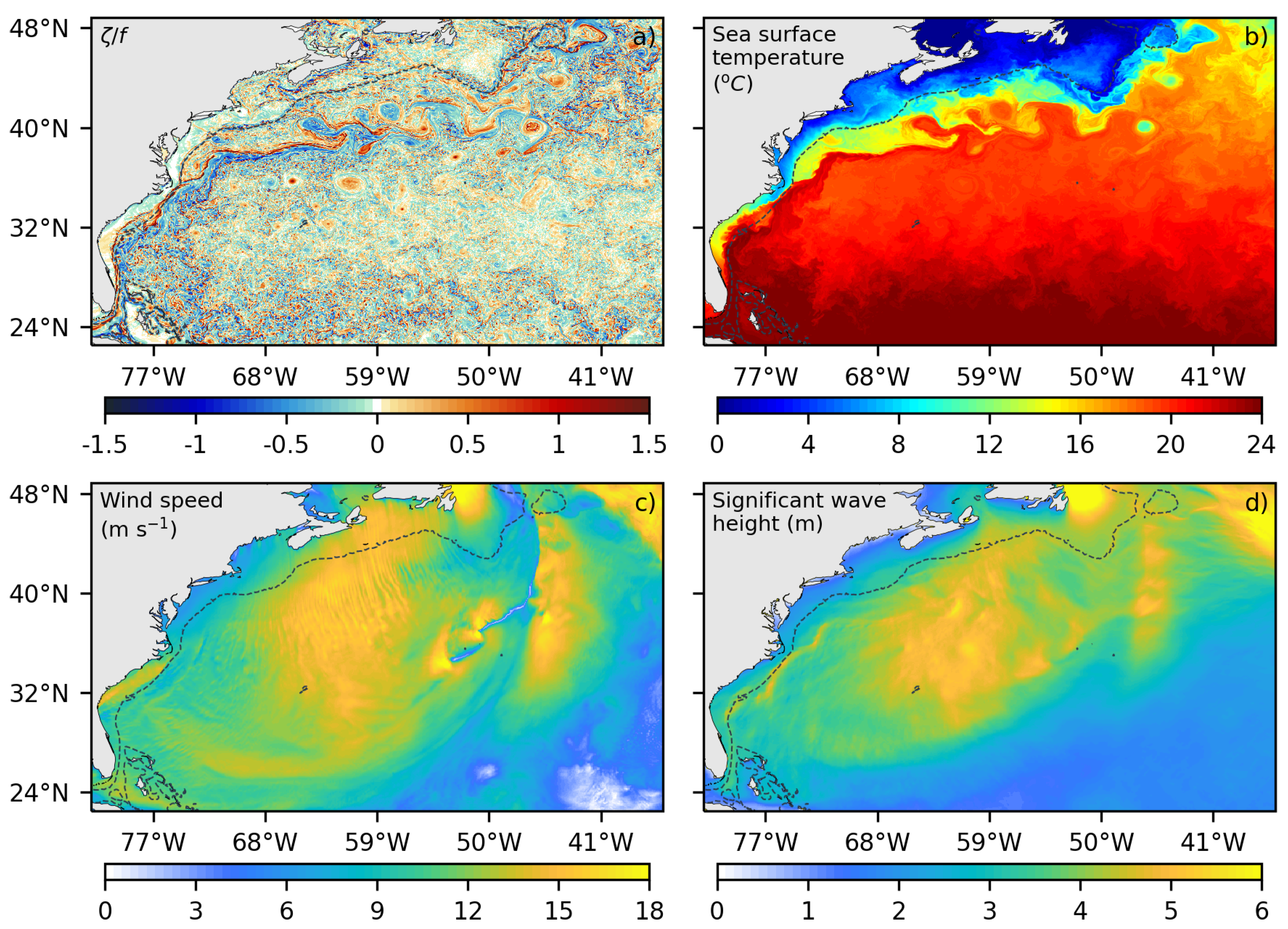
Figure 2.
Coupling strategy for the CROCO-WW3-WRF system.
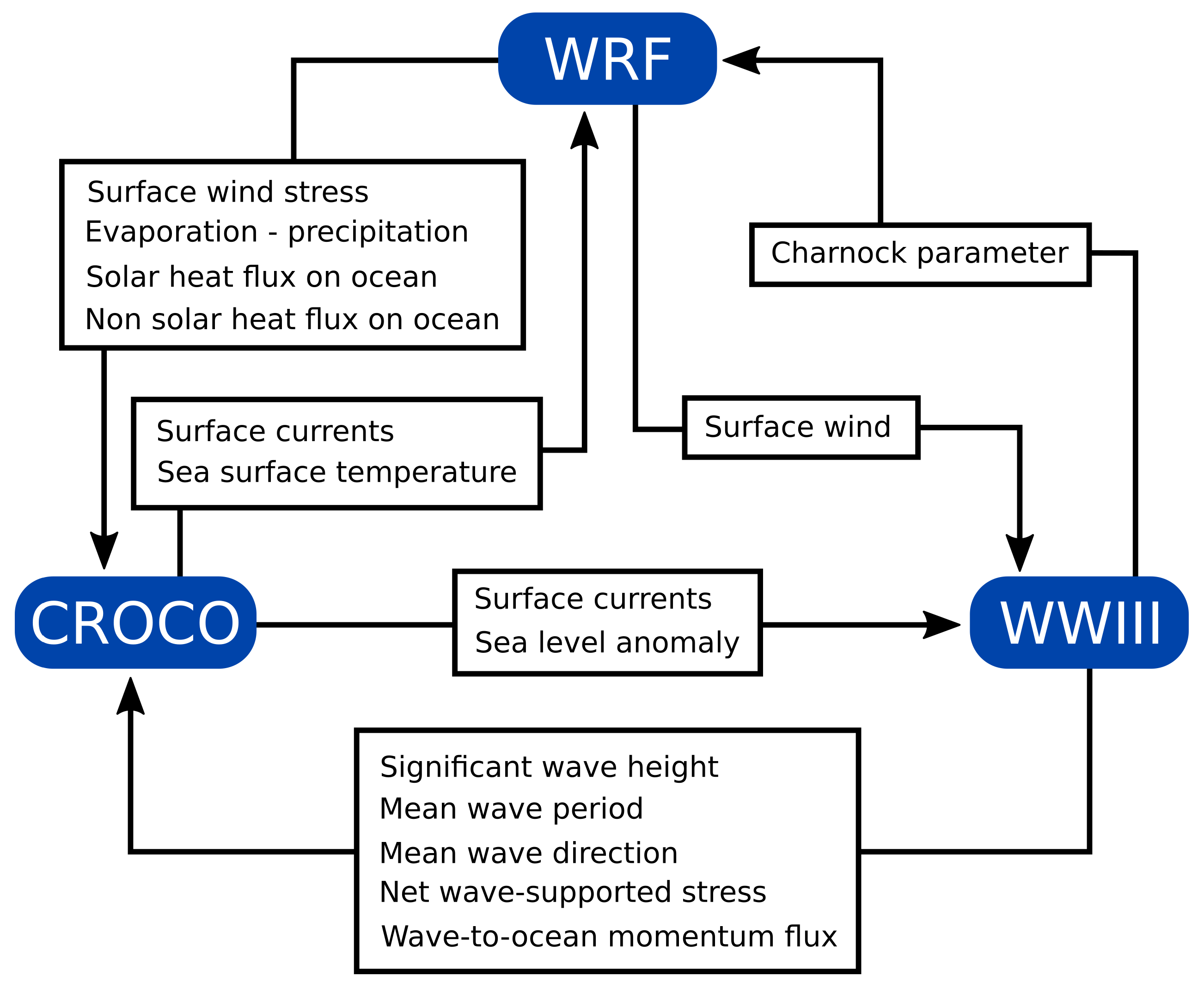
Figure 3.
(a) Probability distribution of wind speeds. The vertical dashed line indicates the 3 m wind speed threshold. (b) Mean noise (colored bars) of surface currents and associated standard deviation (error bars) as a function of wind speed in the ODSL2N dataset. The horizontal dashed line indicates the 50 cm noise threshold.
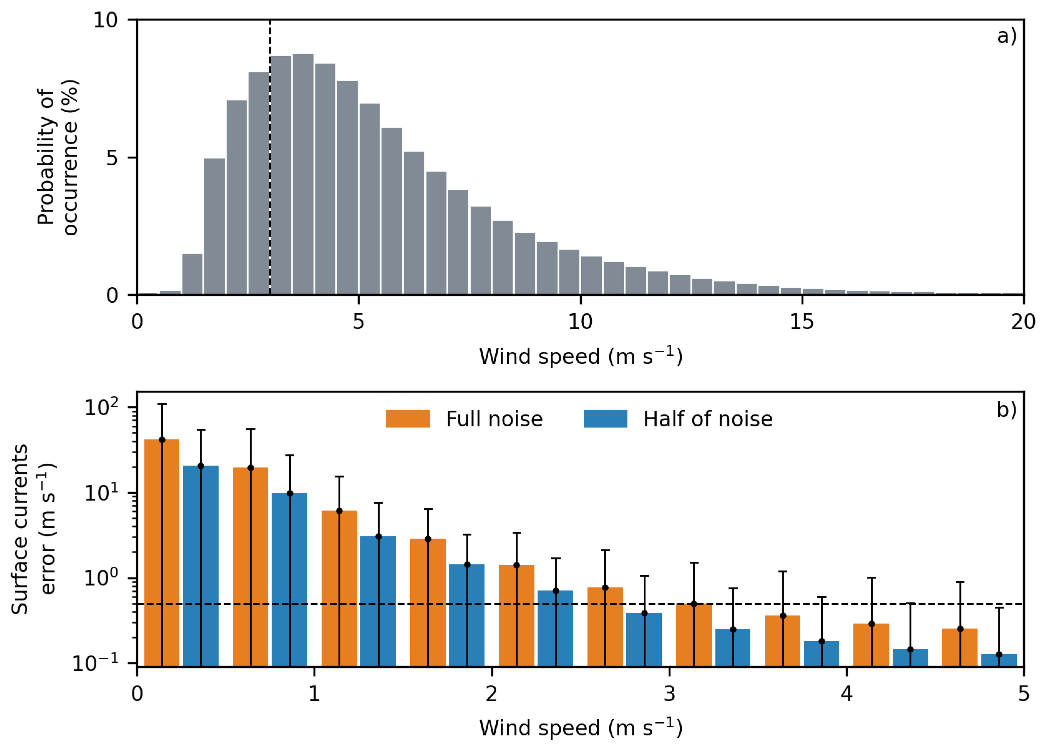
Figure 4.
Comparison of the current speed (first column) and wind stress (second column) from the different datasets obtained through the ODYSEA simulator. Examples for the , , and datasets are shown across different rows.
Figure 4.
Comparison of the current speed (first column) and wind stress (second column) from the different datasets obtained through the ODYSEA simulator. Examples for the , , and datasets are shown across different rows.
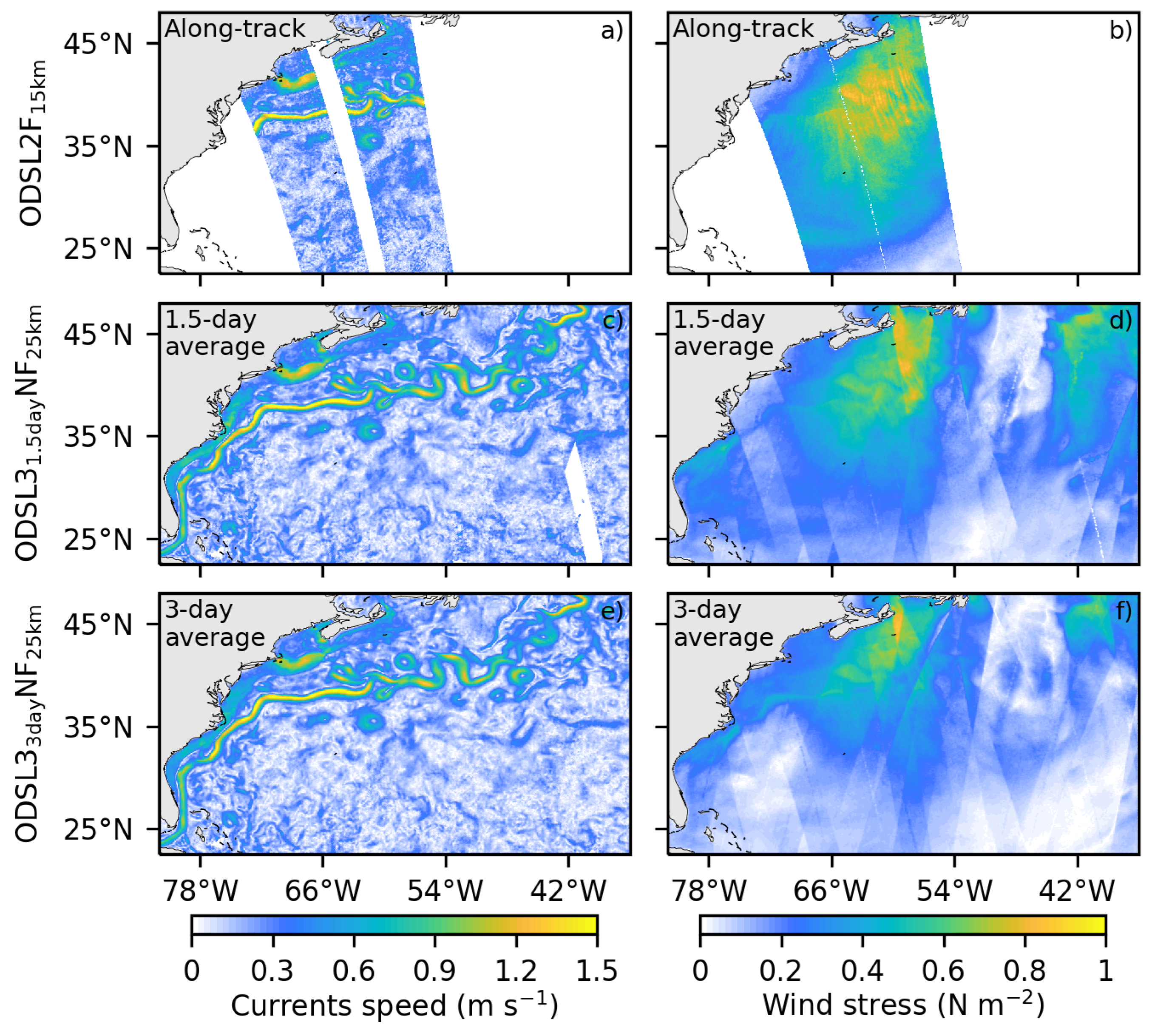
Figure 5.
Mean (first column) and eddy (second column) kinetic over the year 2005 for the reference simulation (first row), (second row), (third row), and QuikSCATlike (fourth row) datasets. The spatially averaged (bars) eddy kinetic energy over the black polygon in b) is depicted for all datasets at the bottom axes. The standard deviation is indicated by the error bars.
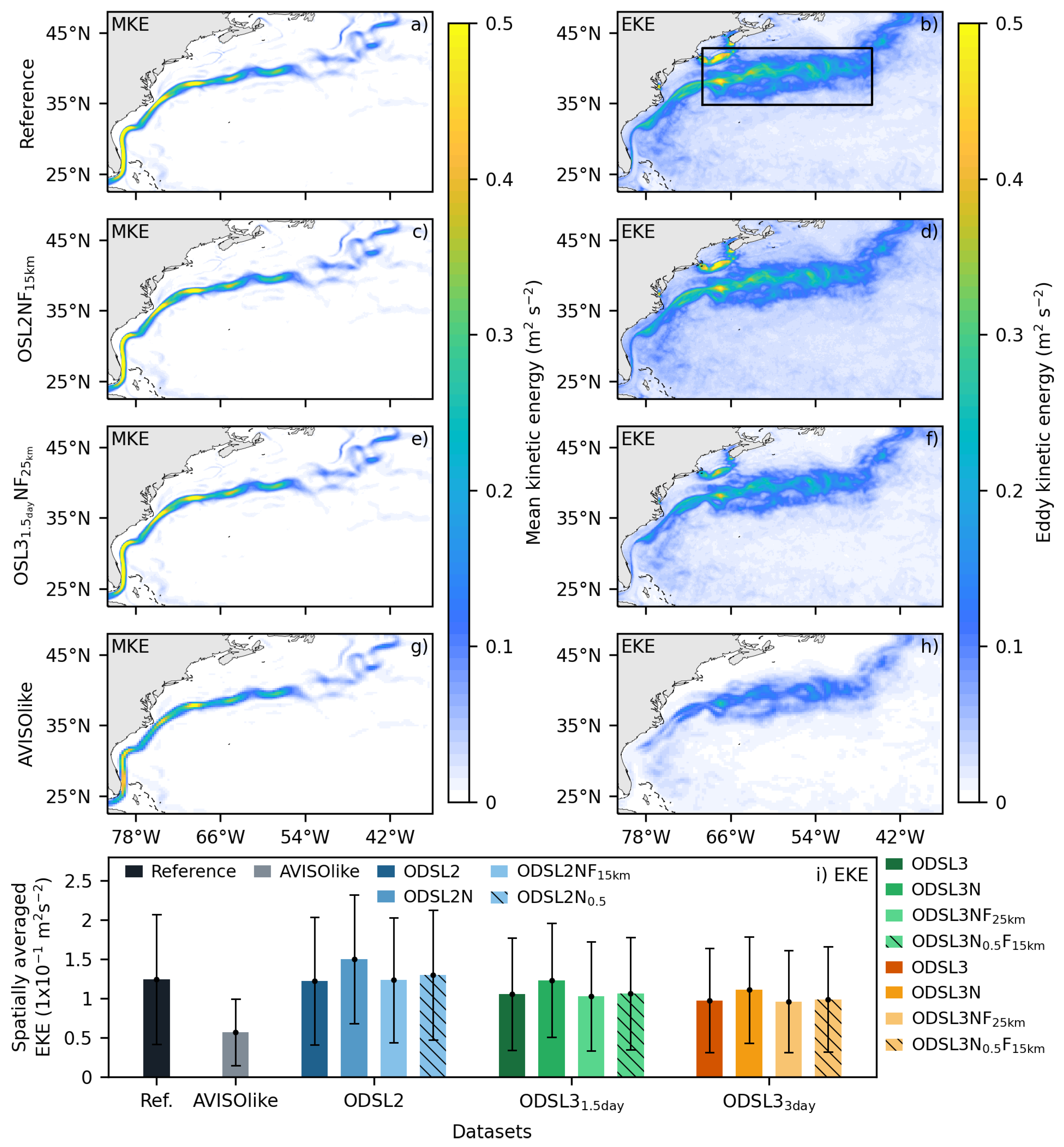
Figure 6.
Kinetic energy wave number spectra estimations for the reference simulation, and the AVISOlike and ODYSEA gridded products over the black polygon depicted in Figure 5a. Theoretical energy dissipation rates of and are depicted with segmented lines in a).
Figure 6.
Kinetic energy wave number spectra estimations for the reference simulation, and the AVISOlike and ODYSEA gridded products over the black polygon depicted in Figure 5a. Theoretical energy dissipation rates of and are depicted with segmented lines in a).
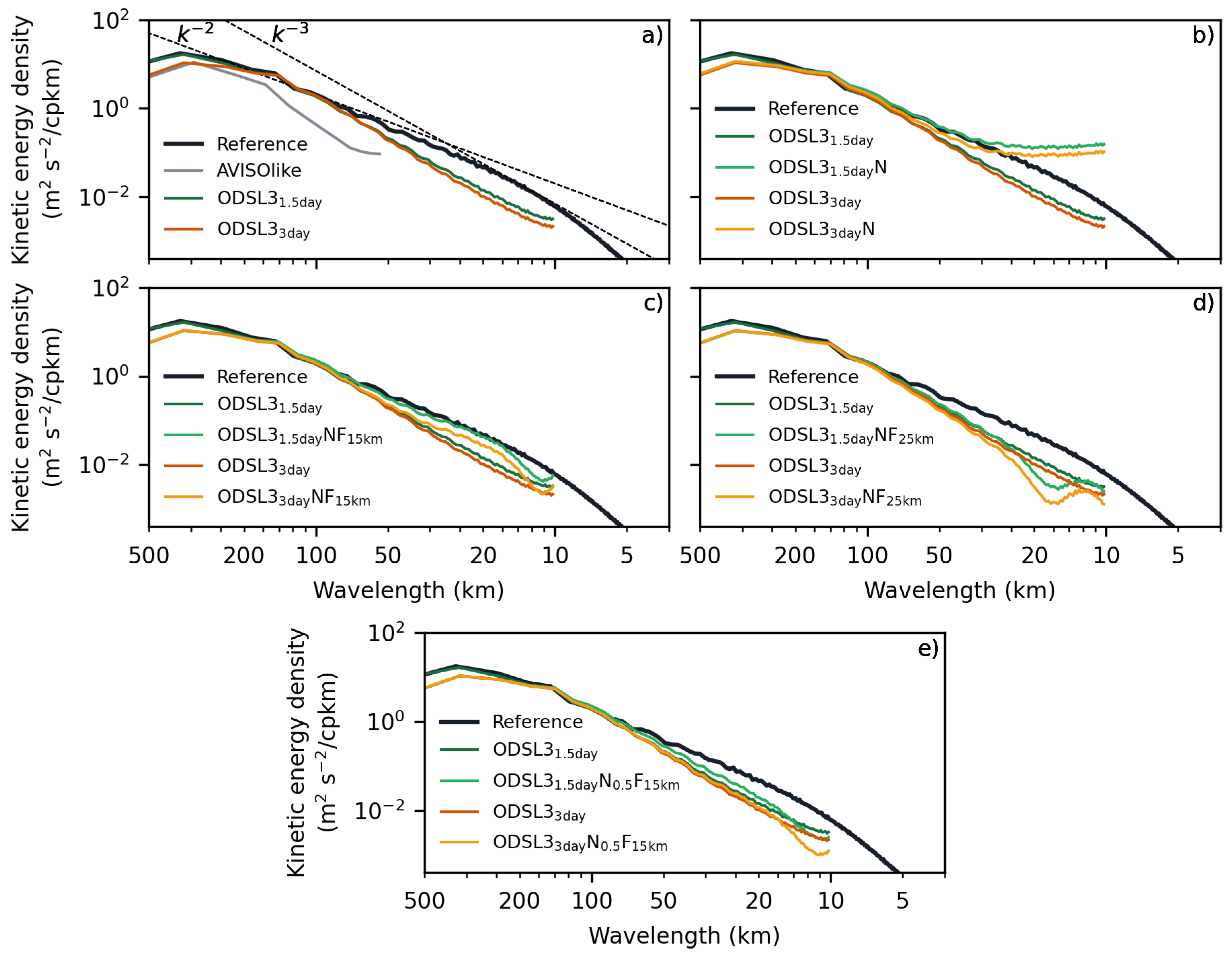
Figure 7.
Mean (first column) and standard deviation (second column) of the wind stress over the year 2005 for the reference simulation (first row), (second row), (third row), and QuikSCATlike (fourth row) datasets. The mean Gulf Stream is depicted by the gray contour in panel b), which represents the 0.1 eddy kinetic energy level. The spatially averaged standard deviation over the black polygon in b) is depicted for all datasets at the bottom axes.
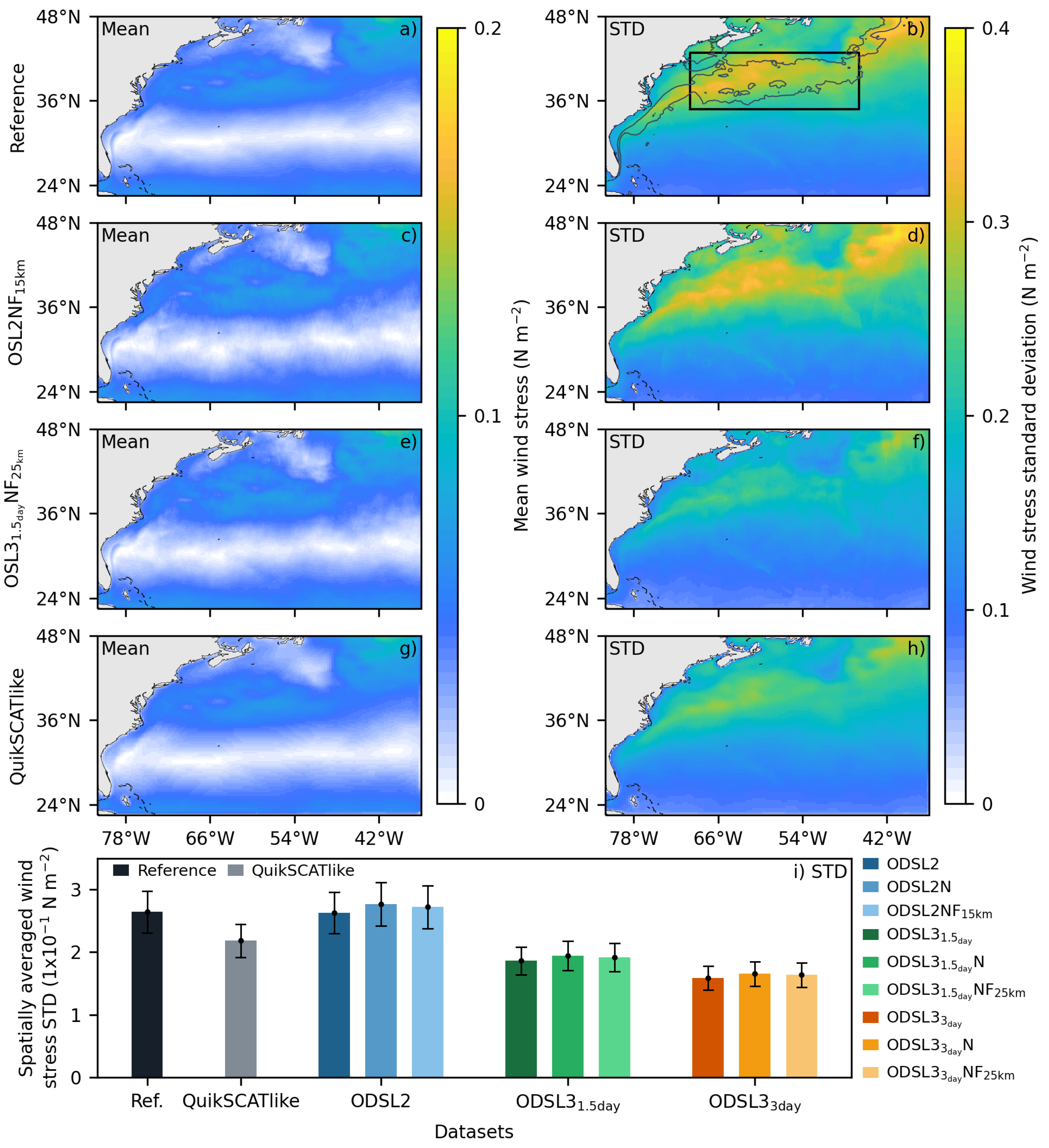
Figure 8.
Cascade of kinetic energy. The Spatially averaged cascade of kinetic energy over the black polygon in b) is depicted for all datasets at the top axes. Spatial distribution of the cascade of kinetic energy at the 20 m (first column) and 150 m (second column) scales for the reference simulation (second row), (third row), (fourth row). Spatial distribution of the cascade of kinetic energy at the 20 m scale for is shown in g), whereas the cascade of kinetic energy at the 150 m scale for AVISOlike is shown in i). The mean Gulf Stream is depicted by the gray contour in panels b) and c), representing the 0.1 eddy kinetic energy level.
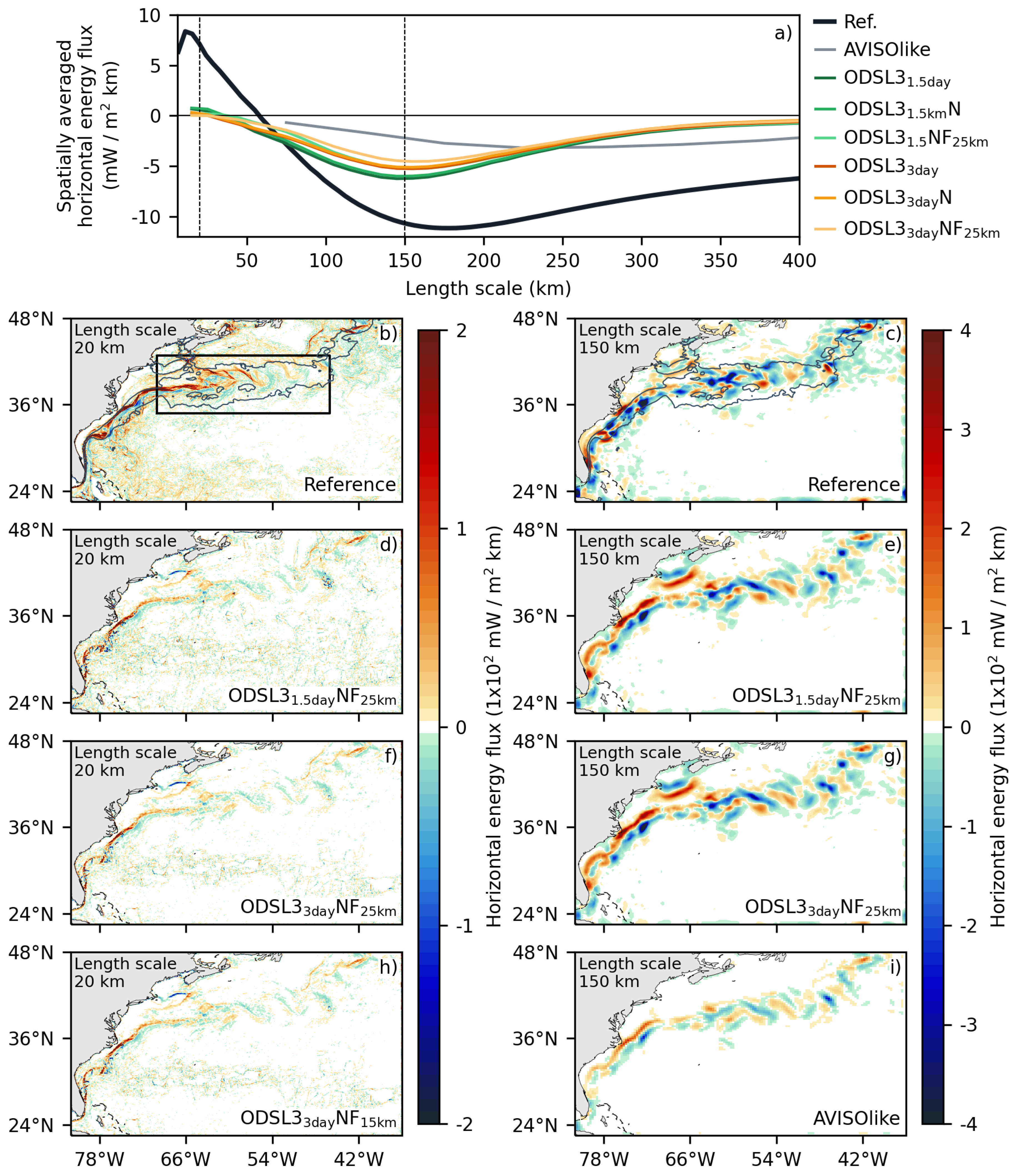
Figure 9.
The spatially averaged wind work over the black polygon in b) is depicted for all datasets at the top panel. Spatial distribution of wind work at the 20 m scale for the reference simulation (b), Obslike (c), (d), and (e). The mean Gulf Stream is depicted by the gray contour in panel b), which represents the 0.1 eddy kinetic energy level.
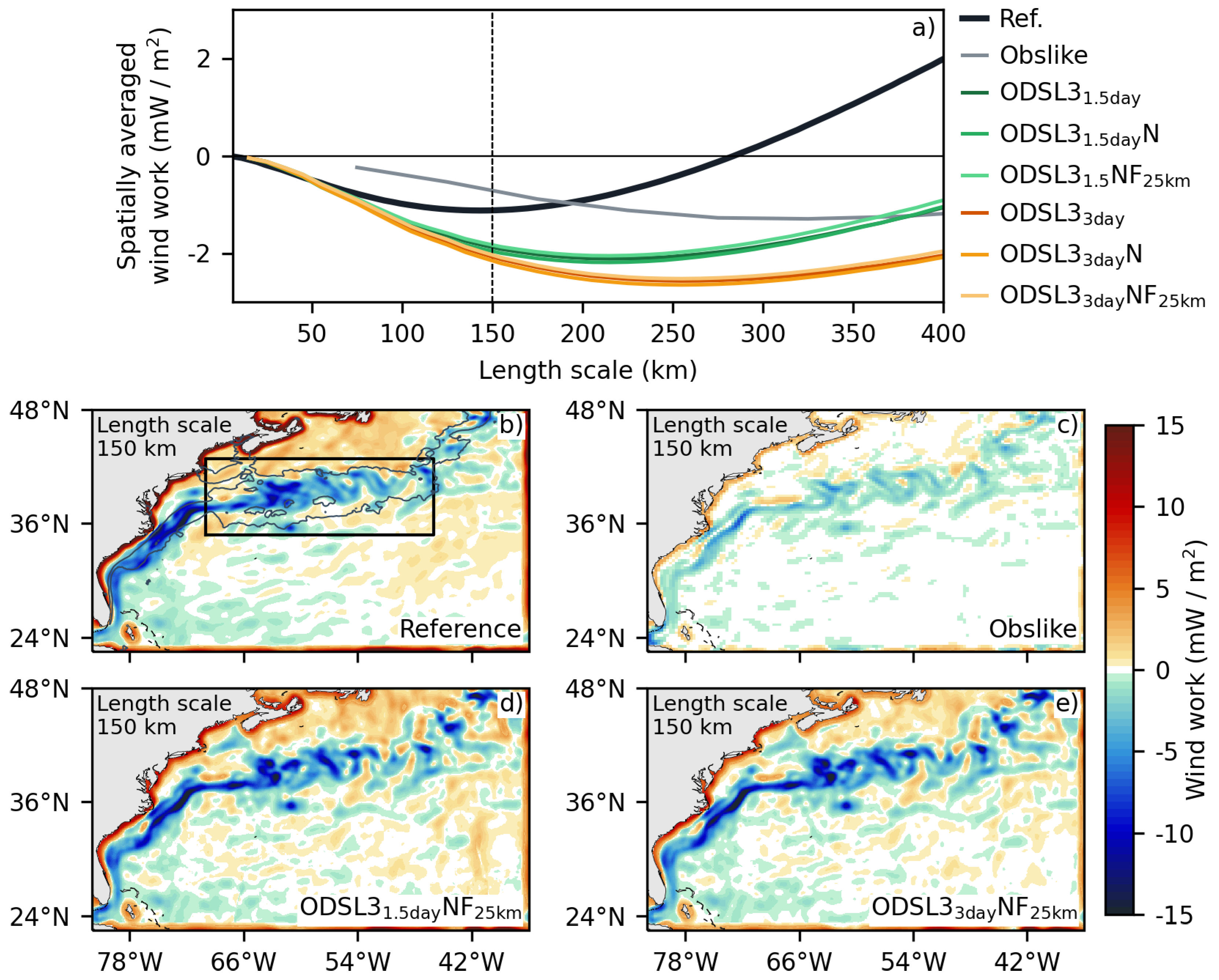
Figure 10.
coupling coefficients for the reference simulation (a) and the Obslike (b) and ODYSEA datasets (c-h). The black contour in a) depicts the mean Gulf Stream position through the eddy kinetic energy contour of 0.1 . The black squared polygon delimits the Loop Current region. Spatially averaged values over the polygon depicted in a) are shown in the bottom panel.
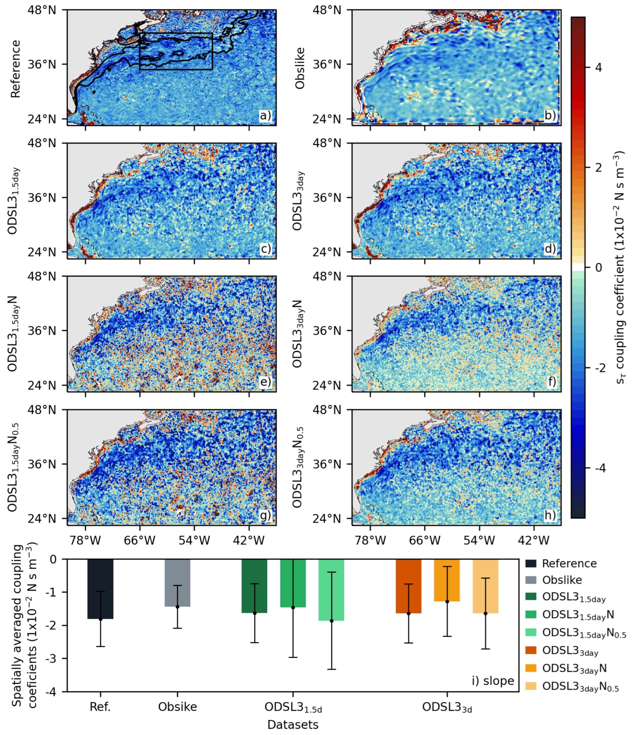

Table 1.
Datasets properties: Noise, temporal filters, and spatial filters.
| Datasets | Noise | Temporal filter | Spatial filter | |||
|---|---|---|---|---|---|---|
| ODSL2 | No | No | No | |||
| ODSL2N | Yes | No | No | |||
| Yes | No | 15 km | ||||
| No | 1.5 days | No | ||||
| N | Yes | 1.5 days | No | |||
| Yes | 1.5 days | 25 km | ||||
| No | 3 days | No | ||||
| N | Yes | 3 days | No | |||
| Yes | 3 days | 25 km |
Table 2.
Time and spatial filters applied to the reference simulation to produce the “like” datasets: AVISOlike, QuikSCATlike, and Obslike. Spatial filter values correspond to the filter diameter.
Table 2.
Time and spatial filters applied to the reference simulation to produce the “like” datasets: AVISOlike, QuikSCATlike, and Obslike. Spatial filter values correspond to the filter diameter.
| Surface currents | Winds and stress | |||
|---|---|---|---|---|
| Datasets | Temporal filter | Spatial filter | Temporal filter | Spatial filter |
| AVISOlike | 7 days | 85 km | – | – |
| QuikSCATlike | – | – | 1 day | 100 km |
| Obslike | 7 days | 85 km | 1 day | 100 km |
Disclaimer/Publisher’s Note: The statements, opinions and data contained in all publications are solely those of the individual author(s) and contributor(s) and not of MDPI and/or the editor(s). MDPI and/or the editor(s) disclaim responsibility for any injury to people or property resulting from any ideas, methods, instructions or products referred to in the content. |
© 2024 by the authors. Licensee MDPI, Basel, Switzerland. This article is an open access article distributed under the terms and conditions of the Creative Commons Attribution (CC BY) license (http://creativecommons.org/licenses/by/4.0/).
Copyright: This open access article is published under a Creative Commons CC BY 4.0 license, which permit the free download, distribution, and reuse, provided that the author and preprint are cited in any reuse.


