1. Introduction
Pipeline blockage is a common issue encountered in mining and filling operations. Slurry filling technology, tailored to the unique characteristics of mines in the western regions—such as large volumes of gangue and significant underground void space—optimizes and integrates traditional techniques, including inter-layer grouting, coal mine fire prevention, and long-distance pipeline transport. This results in the development of a new, regionally adaptive, process-matching, and cost-effective slurry filling technology [
1]. The technology has been successfully applied in several coal mines in the Northwestern region, such as Longwang Gou, Huang Ling No. 2, and Bulian Gou coal mines, for gangue slurry treatment. This demonstrates that the technology can effectively address the treatment needs of coal-based solid waste, yielding significant economic and social benefits [
2]. However, the application of this technology also faces the issue of pipeline blockages in the slurry transport system. The technology involves mixing coal-based solid waste with water in a specific ratio, and then preparing a slurry with the required concentration either on the surface or underground for transportation. The slurry is pumped through pipelines, with the remaining voids in the underground mined-out areas serving as the filling location, enabling in-situ filling of solid waste and achieving zero discharge on the surface. Therefore, the slurry transport pipeline is the critical component of this filling technology. However, various factors can lead to pipeline blockages, which reduce the pipe diameter, increase the flow resistance, cause a significant rise in pumping pressure, and decrease the slurry flow rate. In severe cases, insufficient flow velocity may result in complete blockage, preventing continuous and timely filling of the mined-out spaces.
Foreign researchers [
3,
4,
5] have conducted in-depth studies on the detection and localization of pipeline blockages. Zhao Lian and Xu Zhenliang [
6] analyzed the causes of slurry pipeline blockages, focusing on the effects of factors such as flow velocity and slurry concentration on the blockage mechanism. Zhang Qinli et al. [
7] used fault tree analysis to investigate various factors and their logical relationships contributing to filling pipeline blockages, identifying 16 key factors, including improper slurry mix and excessive bends, as the most significant contributors. Han Xuejing et al. [
8] examined the causes of pipeline blockages due to excessive instantaneous slurry flow velocity. Liu Fuming [
9] conducted a CFD simulation to analyze the flow characteristics of slurry in a 90° elbow pipe, investigating the effects of varying velocity and particle size on the particle velocity distribution and volume fraction. The results indicated that at lower velocities, slurry tends to experience phase separation, whereas at higher velocities, the particle distribution becomes more uniform, which is in line with the requirements for long-distance pipeline transportation.In slurry injection pipelines, fluid flow can induce vibrations in the pipe walls due to factors like flow velocity and pressure. Using Distributed Acoustic Sensing (DAS) technology, phase-sensitive detection allows for the monitoring of these vibrations. To assess the impact of the internal fluid flow on pipe wall vibrations, Computational Fluid Dynamics (CFD) simulations using FLUENT software have been employed to analyze the pressure and velocity distribution characteristics of the slurry in the pipeline under different blockage scenarios. This approach aims to alleviate the blockage issues encountered in slurry transportation.
2. Long-Distance Gangue Slurry Ring Tube Experiment
2.1. Test System
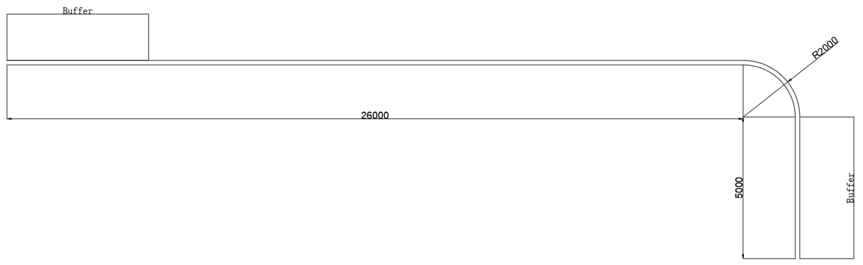
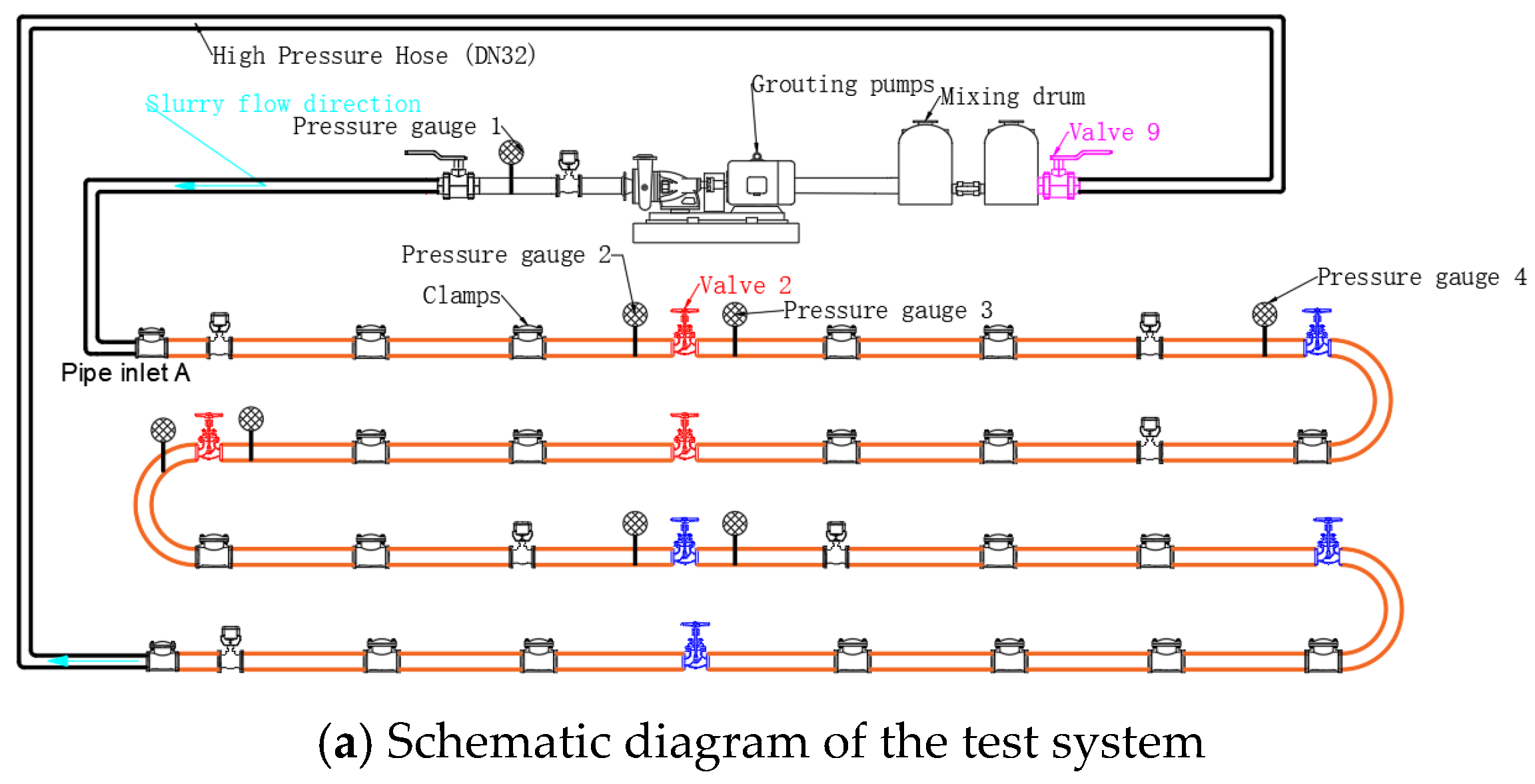
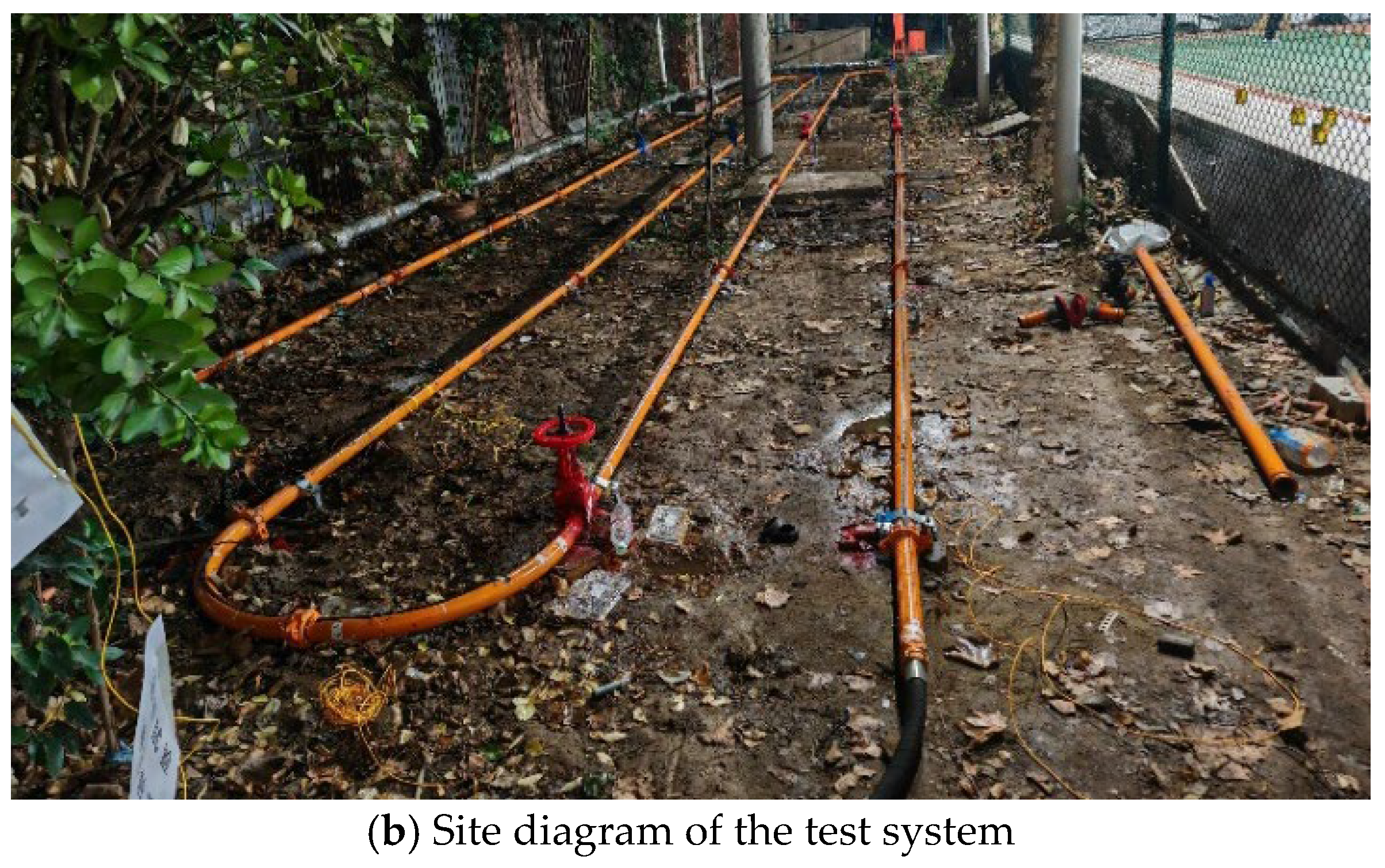
This experiment focuses on the physical simulation of the straight pipe section within the underground slurry filling and transport system, using adjacent and low-position grouting techniques. A tailings slurry transport system was constructed utilizing the existing grouting pump and pipeline setup. The system consists of a slurry storage tank, grouting tank, grouting pump, flow meter, pressure gauge, valves, and grouting pipeline.
The total length of the experimental system is 130.71 meters, comprising 89.71 meters of grouting pipeline and 40 meters of high-pressure rubber hose. The grouting pipeline is made up of 28 straight pipes (3 meters in length), 3 elbow pipes (1 meter in length), and 2 connecting pipes (0.5 meters in length). These components are arranged into 4 rows, each containing 7 straight pipes, as shown in
Figure 1.
The grouting pump is a critical piece of equipment in the transport of tailings slurry, as it provides the necessary energy to maintain continuous flow. This experiment utilizes a pressure-based transport method, with the selection of the pump being a key factor. Common types of pumps include reciprocating pumps, centrifugal pumps, and diaphragm pumps. Given the relatively short pipeline and low lifting height in this experiment, and based on hydraulic calculations and system design, the 2ZBY120/15-18.5 type mining hydraulic grouting pump was selected. This pump has a flow rate range of 30–120 L/min and a grouting pressure range of 0–15 MPa.
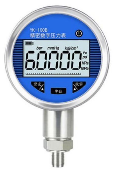
Pressure gauges are employed to monitor the pressure within the pipeline. Pressure gauge 1 measures the initial pressure, while pressure gauges 2 and 3 monitor the pressure variations downstream of the blockage point. The YK-100B digital pressure gauge was chosen for this purpose (see
Figure 2).
2.2. Introduction to Distribution
Based on the experimental setup, a Fluent numerical simulation was conducted to model the first row of pipes on-site. The pressures measured by Pressure Gauges 2 and 3 were compared with the corresponding points in the numerical simulation for analysis. The results of this comparison are illustrated in
Figure 1.
2.3. Comparative Analysis of Simulations and Experiments
To validate the fluid characteristics of this experiment, a 1:1 scale numerical simulation of the slag slurry was conducted using ANSYS. A comparison of the simulation results was then performed.
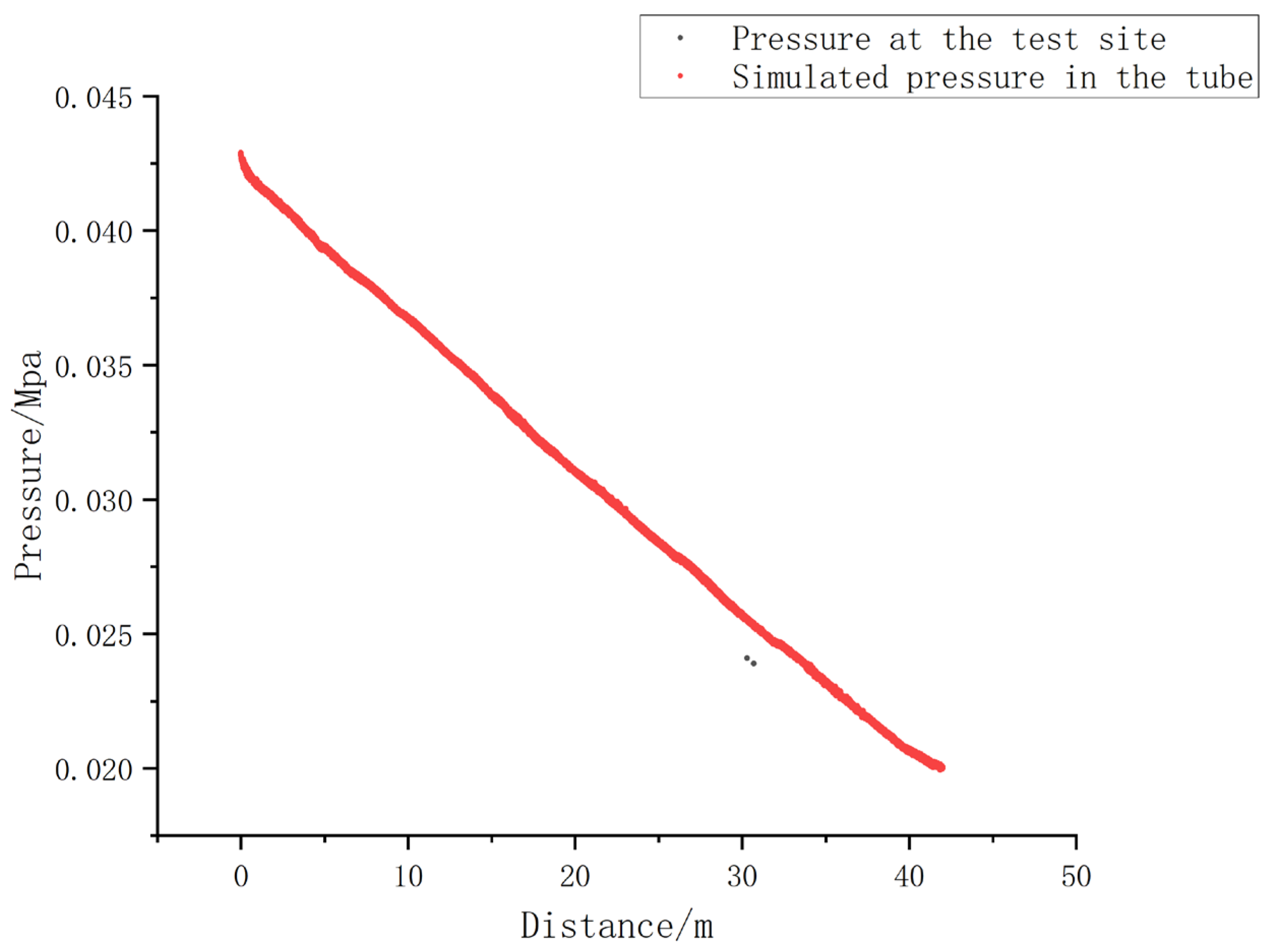
As shown in
Figure 3, the pressure distribution obtained from the software simulation closely aligns with the results calculated using theoretical formulas. Comparing the pressure values from Pressure Gauges 2 and 3 with the simulation data, the agreement is satisfactory, with the error remaining within 6%. This indicates that the on-site experimental measurements are relatively accurate.
3. Establishment of a Grouting Pipeline Blockage Model
3.1. Establishment of Gangue Pipeline Blockage Form
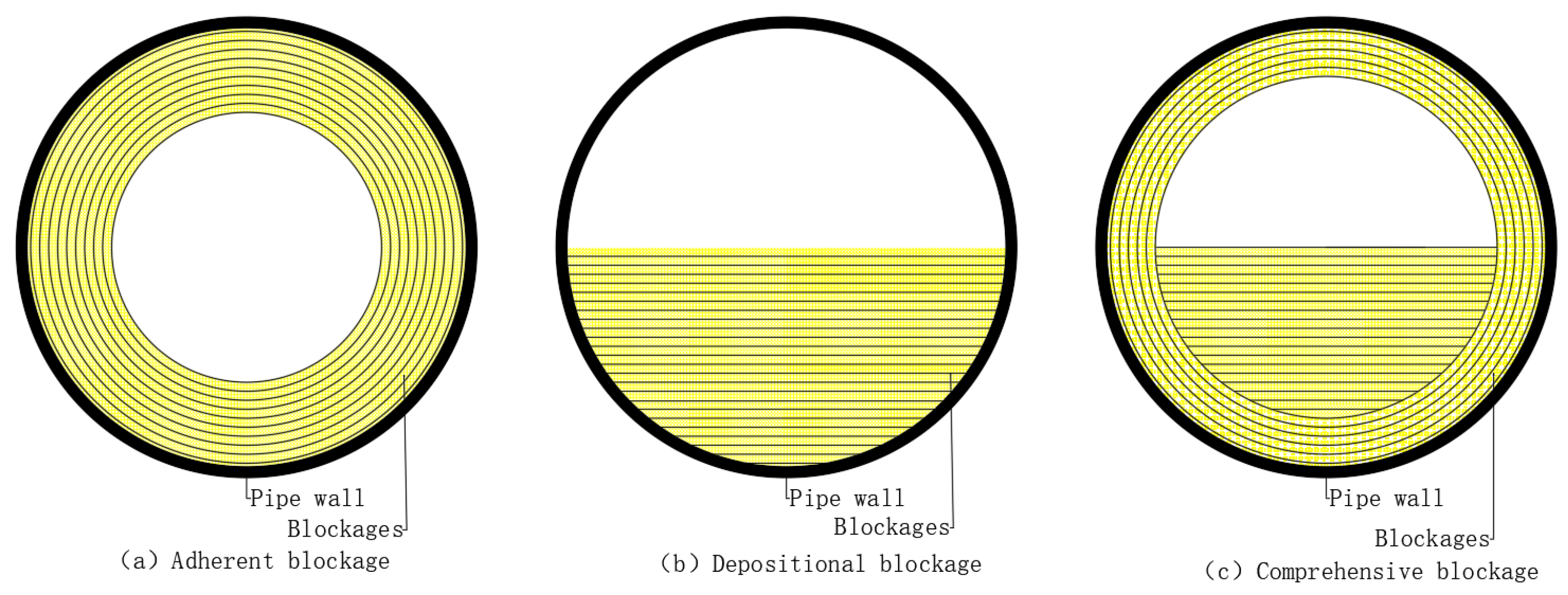
Based on the process of blockage formation in the on-site grouting pipeline, blockages can be classified into attachment-type blockages, deposition-type blockages, and composite blockages, as shown in
Figure 4 [
10]. Furthermore, according to the cause and nature of the blockage, they can be categorized into partial blockages and complete blockages. Partial blockages can be further divided into single blockages and multiple blockages [
11].
In actual grouting pipeline blockages, most blockages are partial rather than complete. The shape and distribution of the blocking material are irregular and unpredictable. In this study, the simulations focus on three specific types of blockages: attachment-type, deposition-type, and composite blockages. To preserve the integrity of characteristic parameters and minimize the complexity of subsequent model calculations, the irregular shape of the blocking material within the pipeline is simplified and approximated to a regular shape, as shown in
Figure 5 [
12].
In the figure, S0 represents the cross-sectional area of the grout pipeline, in square meters (m2); S2 represents the cross-sectional area of the pipeline segment affected by blockage, also in square meters (m2); L1 is the distance from the start of the pipeline to the beginning of the blocked section, in meters (m); L2 is the length of the blocked segment in the pipeline, in meters (m); and L is the total simulated length of the grout pipeline, in meters (m).
To thoroughly investigate the flow characteristics of the grout in the injection pipeline, a 1:1 scale three-dimensional model of the grout pipeline and blockage scenario was established using ANSYS software. The length of the pipeline in the grout filling system varies, and during numerical simulations, a buffer zone is typically incorporated to ensure that the grout flows adequately through the pipeline. In the experiment, an extra horizontal section of 3m to 5m is chosen as the buffer zone. In this study, a 5m long straight pipe is selected as the buffer zone.
Based on the field conditions, this study simulates a 21m long horizontal straight pipe and a 90° elbow with a 2m bending radius, using 16Mn wear-resistant seamless steel pipes. The three-dimensional physical model of the grout pipeline, with different blockage locations and degrees of blockage, is established as shown in
Figure 6. The experiment primarily utilizes SolidWorks to create the 3D geometric model, with the fluid inside the pipe being filled using the Volume Extraction command. The ANSYS-MESHING module is then employed to generate the mesh for the fluid inside the pipeline, ensuring accurate simulation of the fluid flow. Due to the relatively simple pipeline structure, the mesh generation prioritizes the use of hexahedral elements for accuracy and computational efficiency. In areas with irregular shapes, such as blockage locations, tetrahedral elements are used. This choice is made because hexahedral meshes offer better quality, faster convergence, and lower computational costs, while tetrahedral meshes are more adaptable, efficiently filling complex geometric shapes. Additionally, mesh refinement is applied near the pipe wall, the blockage region, and the inlet and outlet areas. The use of hexahedral meshes yielded good results, with the total number of mesh elements ranging from 1.29 million to 1.4 million. Finally, mesh quality was evaluated using the Skewness criterion, which indicated that the element quality was classified as excellent and good.
Figure 6.
Simulated pipeline distribution diagram.
Figure 6.
Simulated pipeline distribution diagram.
Figure 7.
Simulated pipeline cross-section.
Figure 7.
Simulated pipeline cross-section.
3.2. Establishment of Computational Models
The slurry, as the working medium in the grouting transport system, has a density of 1700 kg/m³, a yield stress of 368.3 Pa, and a viscosity of 0.5 Pa·s. Before establishing the computational model, the flow regime (laminar, turbulent, or transitional flow) of the slurry in the circular pipeline can be determined using the Reynolds number. The Reynolds number is calculated using the following equation [
12]:
In the equation, ρ represents the fluid density, v is the average velocity at the cross-section, μ denotes the dynamic viscosity of the fluid, and d refers to the inner diameter of the filling pipeline.
Given that the density of the filling slurry is 1700 kg/m³, the pipeline transport velocity is selected as 2 m/s, and the diameter of the transport pipeline is 0.16 m.
The critical Reynolds number for a Newtonian fluid is 2100. For non-Newtonian Bingham slurry in engineering applications, the critical Reynolds number is variable and generally exceeds 2100. Therefore, the flow within the slurry pipeline remains in a laminar state. The motion of any substance must satisfy the mass conservation equation, which, in a Cartesian coordinate system, is expressed as:
Equation for Conservation of Fluid Mass:
Particle Mass Conservation Equation:
In the equation, ρ represents the fluid density; xi is the coordinate component in the i-direction; and ui denotes the velocity in the i-direction.
Where:
xi refers to the Eulerian coordinates, with i=1,2,3;
ρ represents the liquid phase density;
represents the solid phase density;
is the velocity vector of the liquid phase;
denotes the velocity vector of the solid phase;
is the turbulent diffusion coefficient.
During the motion of the fluid, the momentum conservation equation also applies. Essentially, the momentum equation follows Newton’s second law, which states that the rate of change of momentum at a fluid node is equal to the sum of all external forces acting on that node. The equation is expressed as:
where:
represents the shear stress tensor;
μ denotes the shear viscosity;
indicates the momentum exchange between the solid and liquid phases;
represents the overall viscosity of the solid phase.
3.3. FLUENT Software Settings
FLUENT is a commonly used computational fluid dynamics (CFD) [
14,
15,
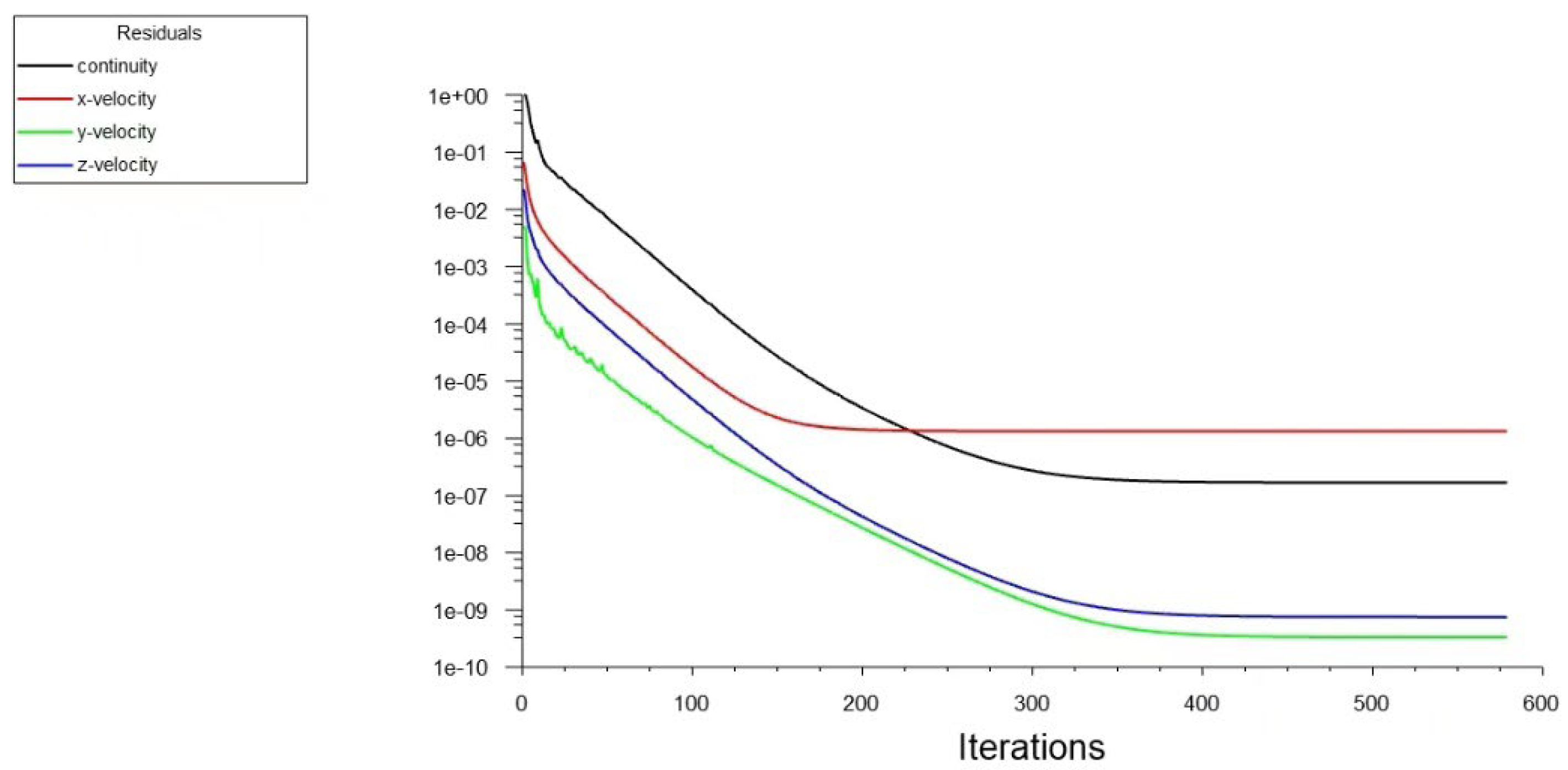
16]software for simulating fluid flows, heat transfer, and chemical reactions. It can provide results that closely approximate experimental findings and reflect the overall characteristics of fluid motion, such as flow velocity, pressure, and other dynamic parameters. This study investigates the flow behavior of slurry in injection pipelines, where the pipeline temperature is approximately 20°C. Since the filling slurry is a multiphase complex fluid containing gas, liquid, and solid phases, and it behaves as a non-Newtonian Bingham plastic, the slurry maintains its homogeneity and uniformity during pipeline transport without segregation or layering. As a simplification, the slurry flow is assumed to be single-phase. The semi-implicit method for pressure-coupling equations is selected. The inlet is set as a velocity inlet with an inflow velocity of 2 m/s, and the outlet is set as a pressure outlet with a static pressure of 10,100 Pa (relative pressure under atmospheric conditions). To verify the accuracy of the simulation model and computational precision, a residual monitoring window is set, and the residual curve is shown in
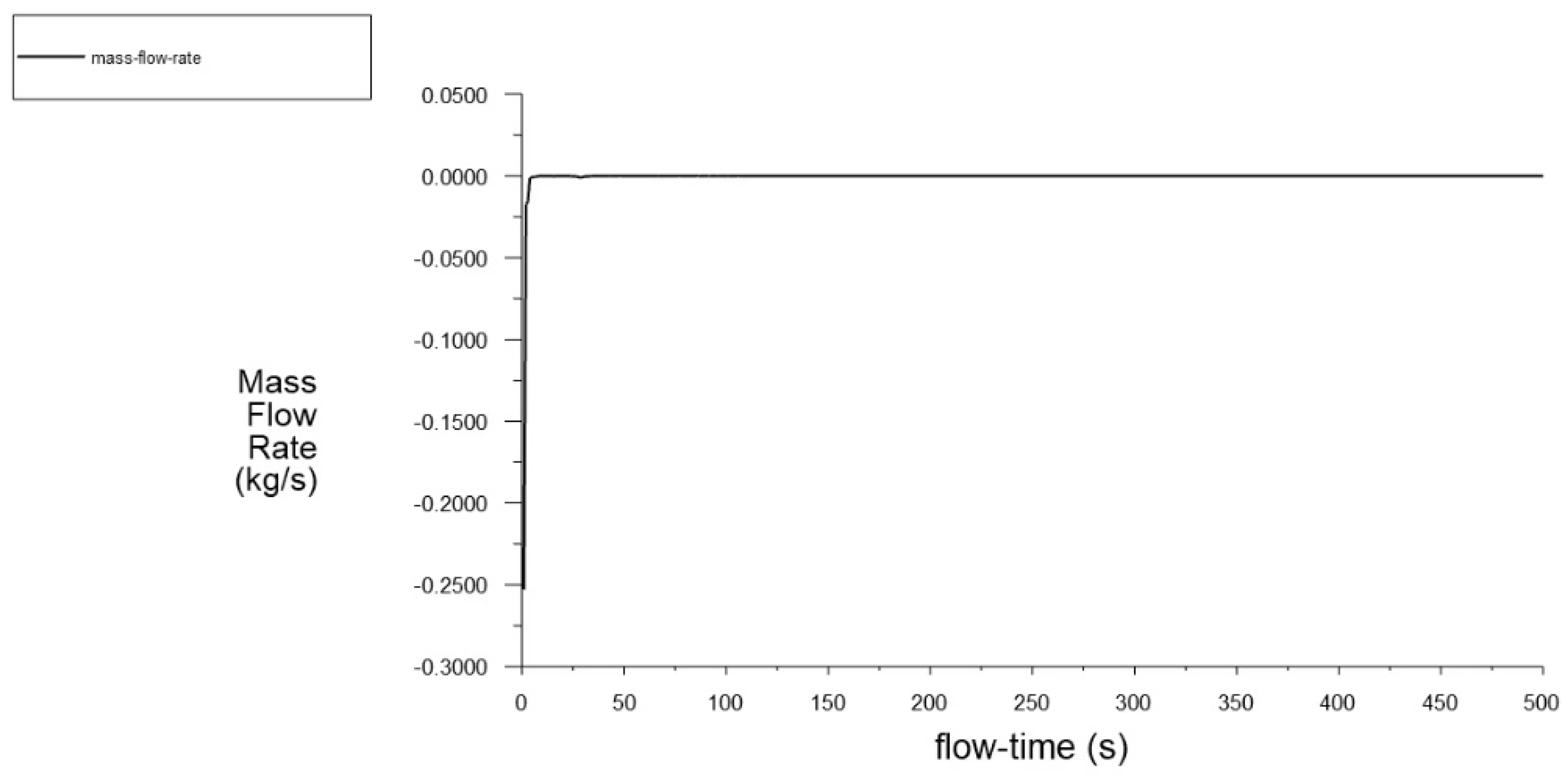
Figure 8. After fluid initialization, the iteration step is set to 600 steps for computation. During the iterations, the residual curves for each condition converge, and the flux conservation at the inlet and outlet approaches zero, as shown in
Figure 9. This indicates that the simulation model closely represents the actual slurry blockage scenarios. The slurry is modeled as a non-Newtonian Bingham fluid, specifically using the H-B model. The slurry density is set to 1700 kg/m³, and the H-B model parameters are configured as follows: the exponent is set to 1, the critical shear stress is 100 r/s, the apparent viscosity is 165.6 Pa·s, and the slurry yield stress is 8.277 Pa.
3.4. Simulated Condition Settings
The slurry filling capacity at the Buliangou Coal Mine is 130 m³/h. In this study, the characteristics of slurry flow under pipeline blockage conditions were investigated at a slurry concentration of 70% and a slurry density of 1.7 t/m³. The study focuses on three independent variables: blockage degree, blockage position, and blockage morphology. The aim is to explore the relationship between these variables and the changes in pipeline pressure along the length of the pipeline, as well as the pressure drop between the pipeline inlet and outlet. The blockage degree is categorized into three levels, the blockage morphology is also classified into three levels, and the blockage position is set at two levels—straight pipe and bent pipe. Additionally, a no-blockage condition is included as a control. In total, 19 experimental conditions were designed, as shown in
Table 1.
4. Analysis of CFD Simulation Results
4.1. Analysis of Simulation Results of Non-Clogging Conditions
According to the Bernoulli equation for fluid transport in pipelines, the energy equation for slurry transport in filling systems is given by:
In the equation, P represents the pressure provided by the filling pump at the pipeline inlet (Pa); denotes the slurry density (kg/m³); g is the gravitational acceleration (9.81 m/s²); H refers to the height difference between the pipeline inlet and outlet (m); v is the slurry flow velocity at the outlet (m/s); and I is the total resistance loss in the pipeline (Pa).
Generally, the pipeline resistance loss consists [
17,
18] of two parts: the frictional loss along the straight pipe section Is and the local resistance loss Ib, which is primarily associated with 90° elbows [
19,
20,
21].
The frictional resistance loss Is along the straight pipe section can be expressed as the product of the total length of the straight section Ls and the unit length frictional resistance loss is, as shown in the following equation:
The flow behavior of slurry in pipe bends is more complex, and in the literature, the local losses in the pipe bend section are generally considered in conjunction with the overall frictional resistance losses along the pipe. The local resistance is typically estimated as 10% to 20% of the total resistance loss in the pipeline. As part of the pipeline system, the pipe bend shares the same inner diameter and slurry parameters as the straight sections, and its resistance loss can also be calculated based on the unit length. The unit length local resistance loss ib of the pipe bend is typically expressed as a multiple of the unit length frictional resistance loss
, as follows:
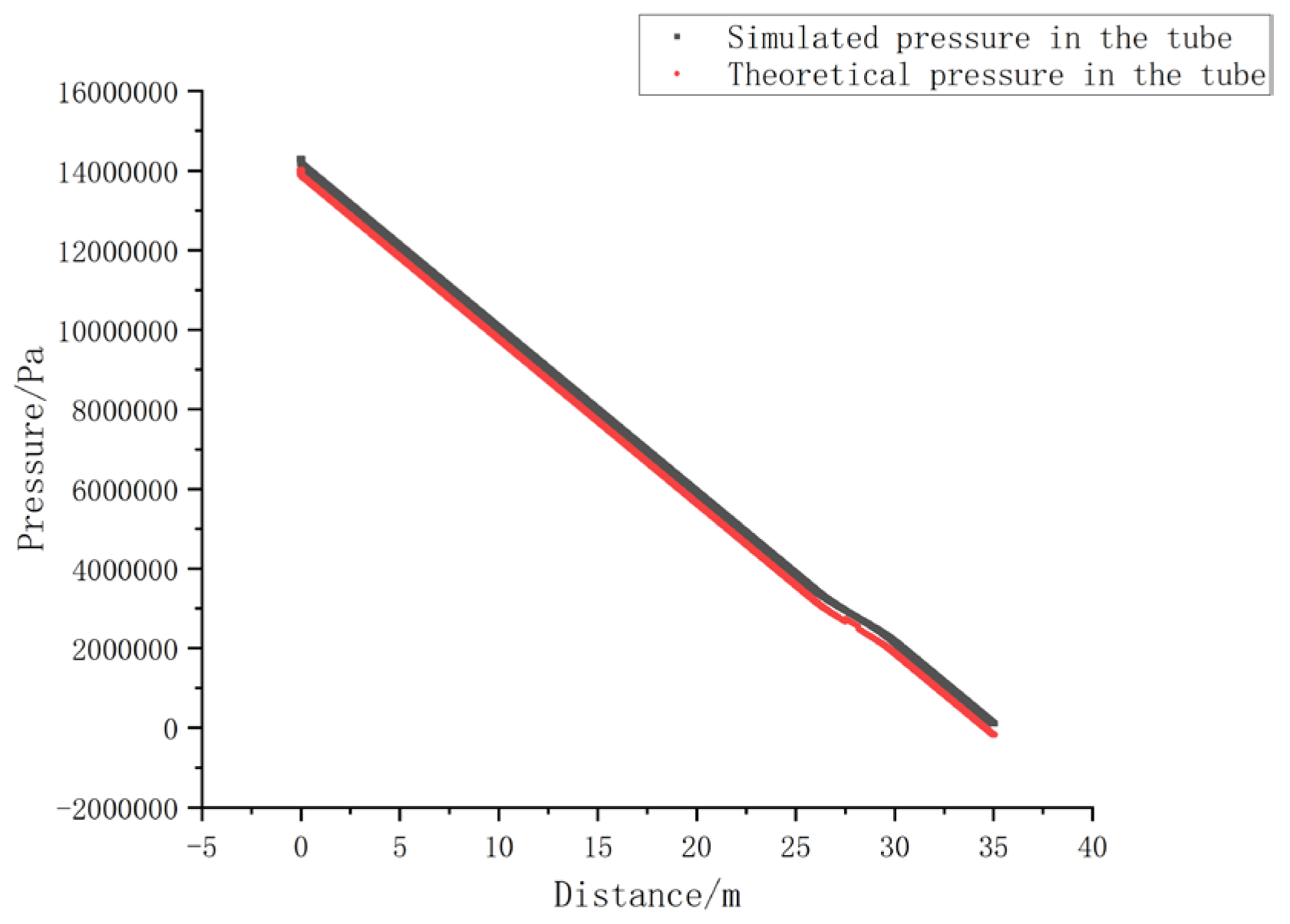
Under the condition of no blockage, the pressure distribution of the pipeline during normal operation is shown in
Figure 10, which includes both the simulation results and theoretical calculations. As shown in
Figure 10, the pressure distribution obtained from the software simulation aligns closely with the theoretical calculation results, and the pressure decreases linearly with increasing pipeline length. Overall, the calculated pressure values and the simulation results are in good agreement, with a deviation of 9.12%. This error primarily arises from the selection of the coefficient kkk at the pipe bend. Due to the complex flow conditions at the bend, it is difficult to accurately determine the kkk value. Nevertheless, it can be concluded that this model design closely reflects the actual operating conditions of the pipeline.
4.2. Analysis of Simulation Results of Blockage Conditions
4.2.1. The Influence of the Degree of Blockage on the Distribution of Pipeline Characteristics
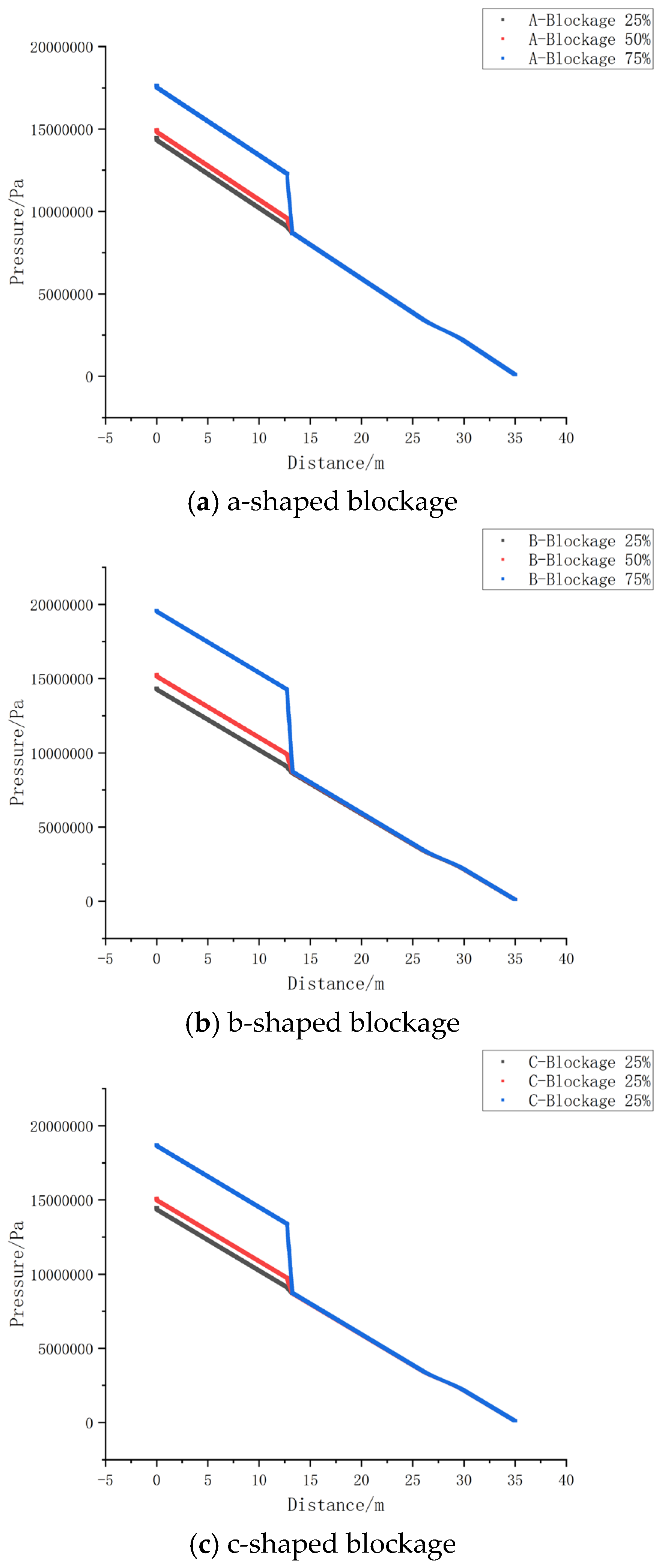
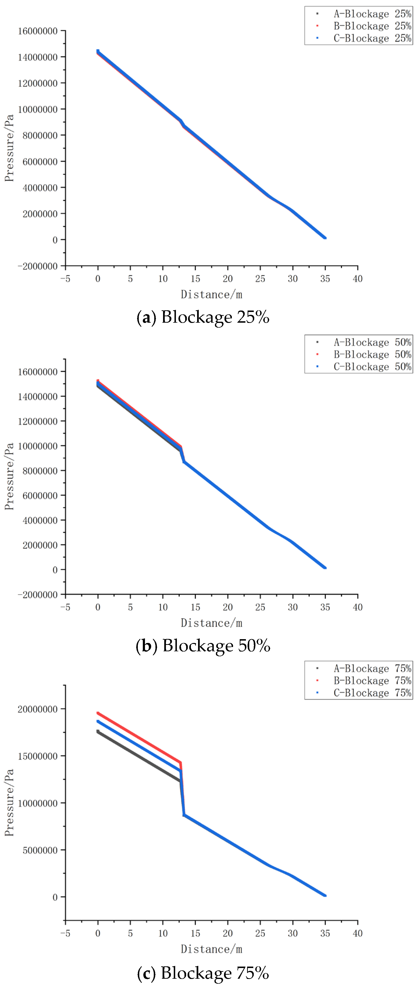
To investigate the relationship between blockage degree and pipeline pressure drop, experimental data under three different blockage shapes were selected. Each set of data corresponds to three levels of blockage: 25%, 50%, and 75%. The pressure along the pipeline for each condition was recorded and compared, as shown in Figure11.
As observed in
Figure 11, the pressure drop increases with the degree of blockage. On the other hand, when the blockage degree is relatively low (i.e., less than 50%), the variation in pressure along the pipeline is minimal, with the maximum pressure drop being only about 3% of the maximum pressure. However, when the blockage degree exceeds 75%, the pressure drop along the pipeline increases sharply, with the minimum pressure drop being over 17% of the maximum pressure. This indicates that the degree of blockage is a significant factor influencing the water flow pressure in the pipeline.
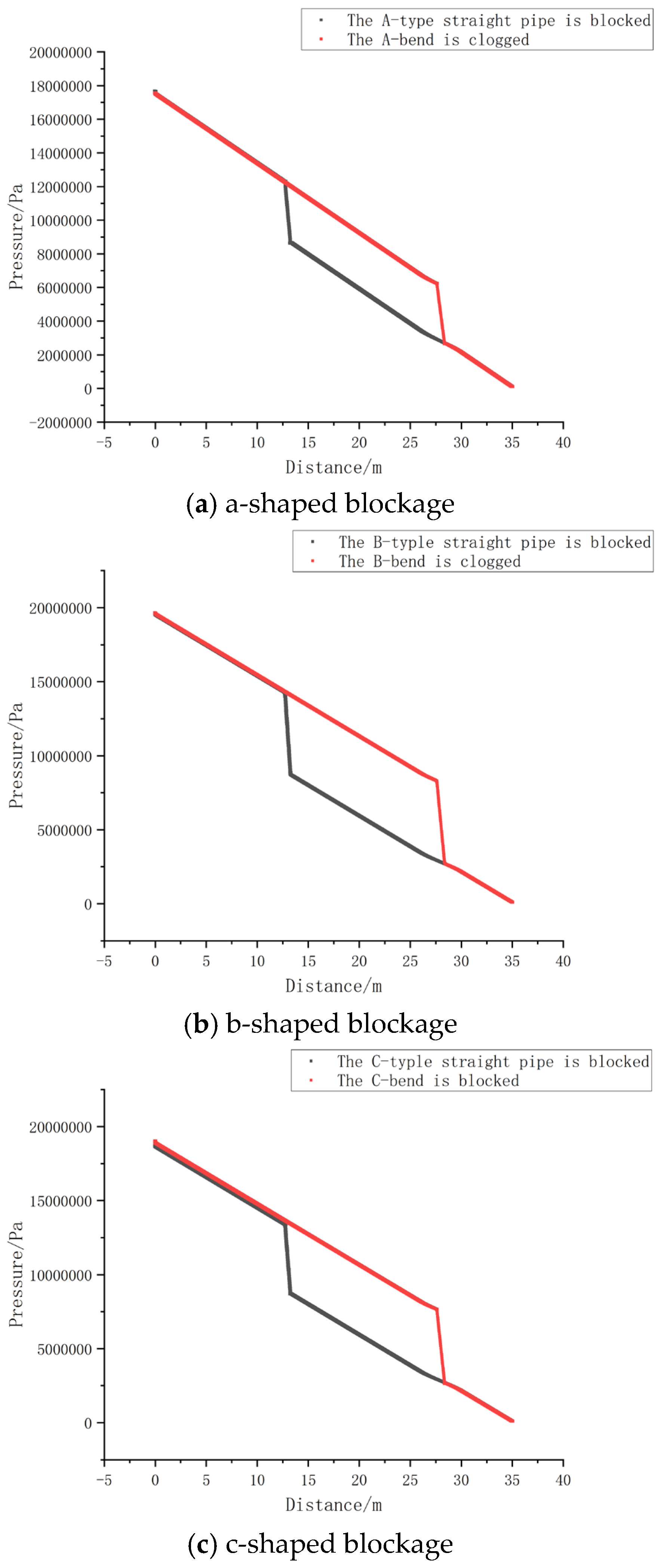
4.2.2. The Influence of Blockage Pattern on the Distribution of Pipeline Characteristics
To investigate the impact of blockage shape on the pressure distribution within the pipeline, three common blockage shapes were simulated under identical conditions, with all other parameters held constant. The pressure variations under different blockage conditions for each blockage shape were compared, as shown in
Figure 12.
As observed in
Figure 12, under a 25% blockage condition, the pressure drop along the pipeline for all three shapes is nearly identical. However, as the blockage degree increases, the pressure drop becomes more pronounced. Notably, the pressure drop for Type B blockage is greater than that for Type C and Type A blockages, with Type C being larger than Type A. Therefore, Type B blockage, which corresponds to deposition-type blockage, presents the most severe hazard.The primary cause of Type B blockage lies in the behavior of the slurry particles inside the pipeline. These particles lose their original balance and, under the influence of gravity, gradually settle to the bottom of the pipeline, forming a deposition-type blockage. As the particles settle, their velocity decreases, eventually coming to a stop due to the frictional resistance at the rough surface of the pipeline. The greater the roughness of the pipe wall, the larger the frictional resistance, and the more likely the particles are to stop, accelerating the formation of deposition-type blockage.To prevent deposition-type blockage, it is recommended to select pipes with smooth inner walls and low roughness when designing slurry injection pipelines.
4.2.3. The Influence of the Blockage Location on the Distribution of Pipeline Characteristics
To investigate the effect of blockage location on the pressure distribution within the pipeline, simulations were conducted for different blockage positions while keeping other parameters constant. The study focused on comparing the pressure drop along the pipeline in straight and bent sections, using experimental data from three different blockage shapes, all under a 75% blockage condition. The results are shown in
Figure 13.
Based on the analysis of
Figure 13, it can be concluded that the variation in blockage location has minimal impact on the pressure distribution. The pressure drop along the straight section of the pipeline decreases approximately linearly, while in the bent section, the pressure follows an arcuate reduction in accordance with the theoretical model. When the blockage occurs at the bend, the pressure first decreases linearly along the arc at the blockage point, then continues to drop along the original curvature of the bend.
Overall, the differences in pressure distribution due to blockage location are insignificant. Whether in straight or bent sections, the pressure drop variations show little distinction. Therefore, compared to blockage degree and blockage shape, the location of the blockage has a smaller effect on the water flow pressure inside the pipeline.
4.2.4. Analysis of the Influence of Flow Velocity Under Blockage Conditions
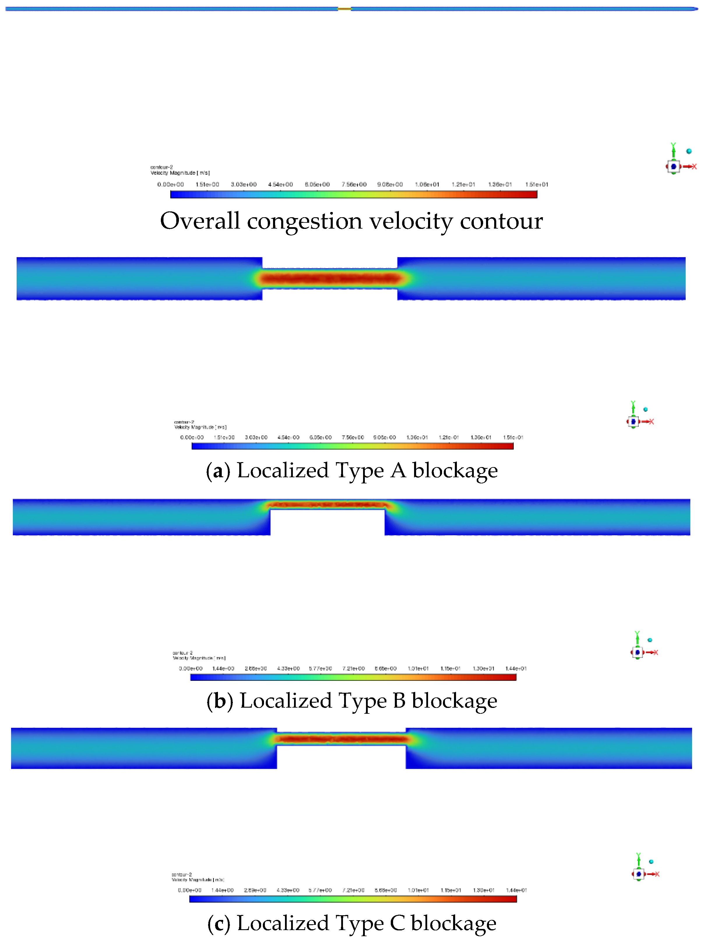
To investigate the impact of the flow velocity factor on fluid flow in the pipeline under three different blockage shapes, data for three blockage degrees—25%, 50%, and 75%—were selected at the center of the pipeline. Velocity contour plots were generated, as shown in
Figure 14.
From
Figure 14, it can be observed that all three blockage shapes lead to a significant increase in flow velocity. Excessively high flow velocities can cause pipe erosion and corrosion, which threatens the safe operation of the pipeline. Below the blockage and in the short section downstream, the flow velocity quickly decreases to near zero, forming a stagnation zone. This condition exacerbates the deposition of solids, thereby worsening the blockage. Notably, in the case of blockage shapes B and C, the stagnation zone area is much larger than that of blockage shape A, indicating that different blockage shapes cause varying levels of disturbance in the subsequent section of the pipeline. Therefore, timely removal of blockages is crucial for the maintenance and management of the grout injection pipeline. To avoid the formation of sedimentation-type and composite blockages, it is advisable to select pipes with smooth inner walls and low roughness during pipeline construction.
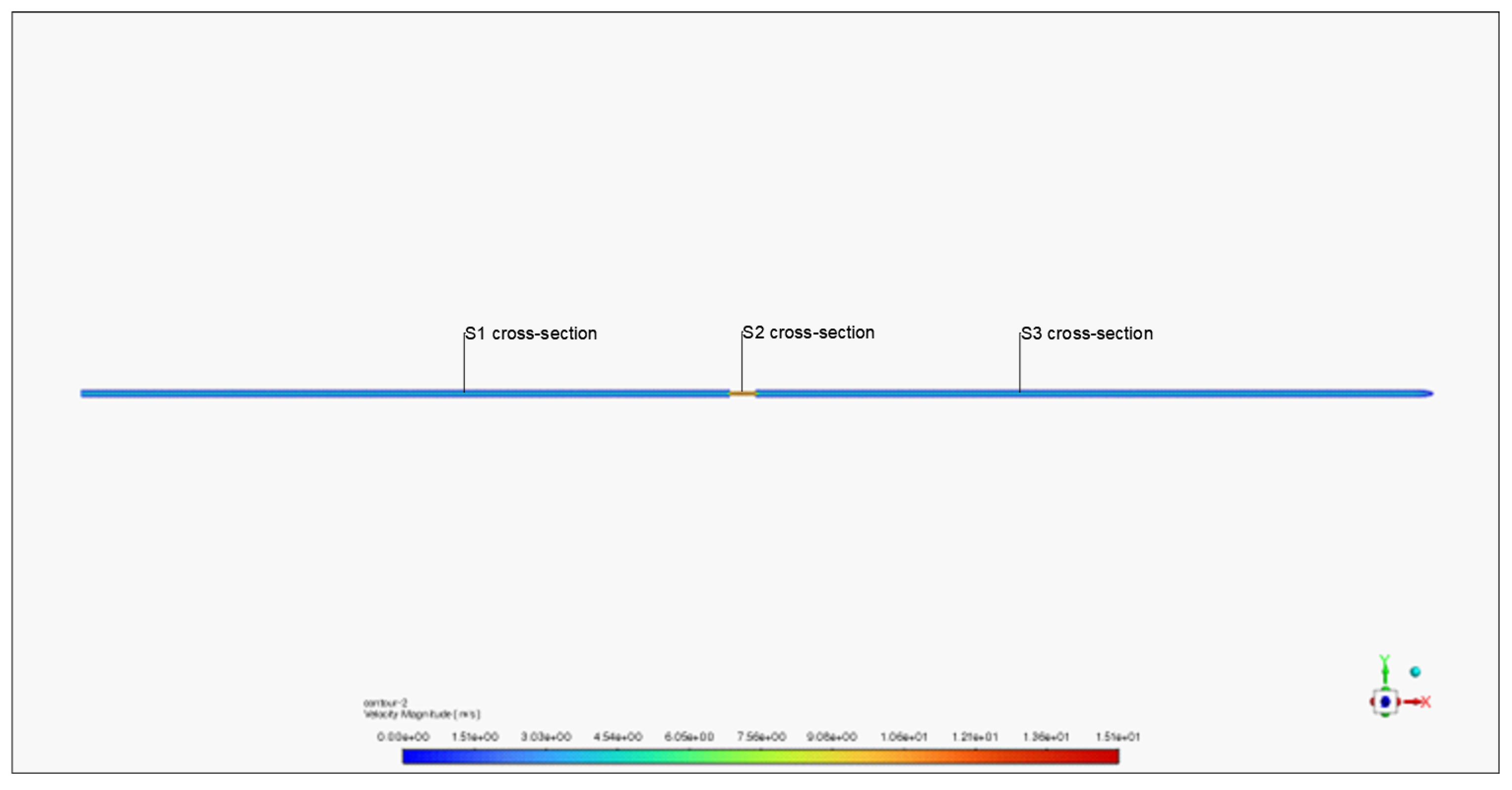
As shown in
Figure 15, this study selects the cross-sections S1, S2, and S3 located at distances of 800mm, 13,000mm, and 18,000mm from the pipeline’s inlet and outlet, respectively, as the sections for the analysis.
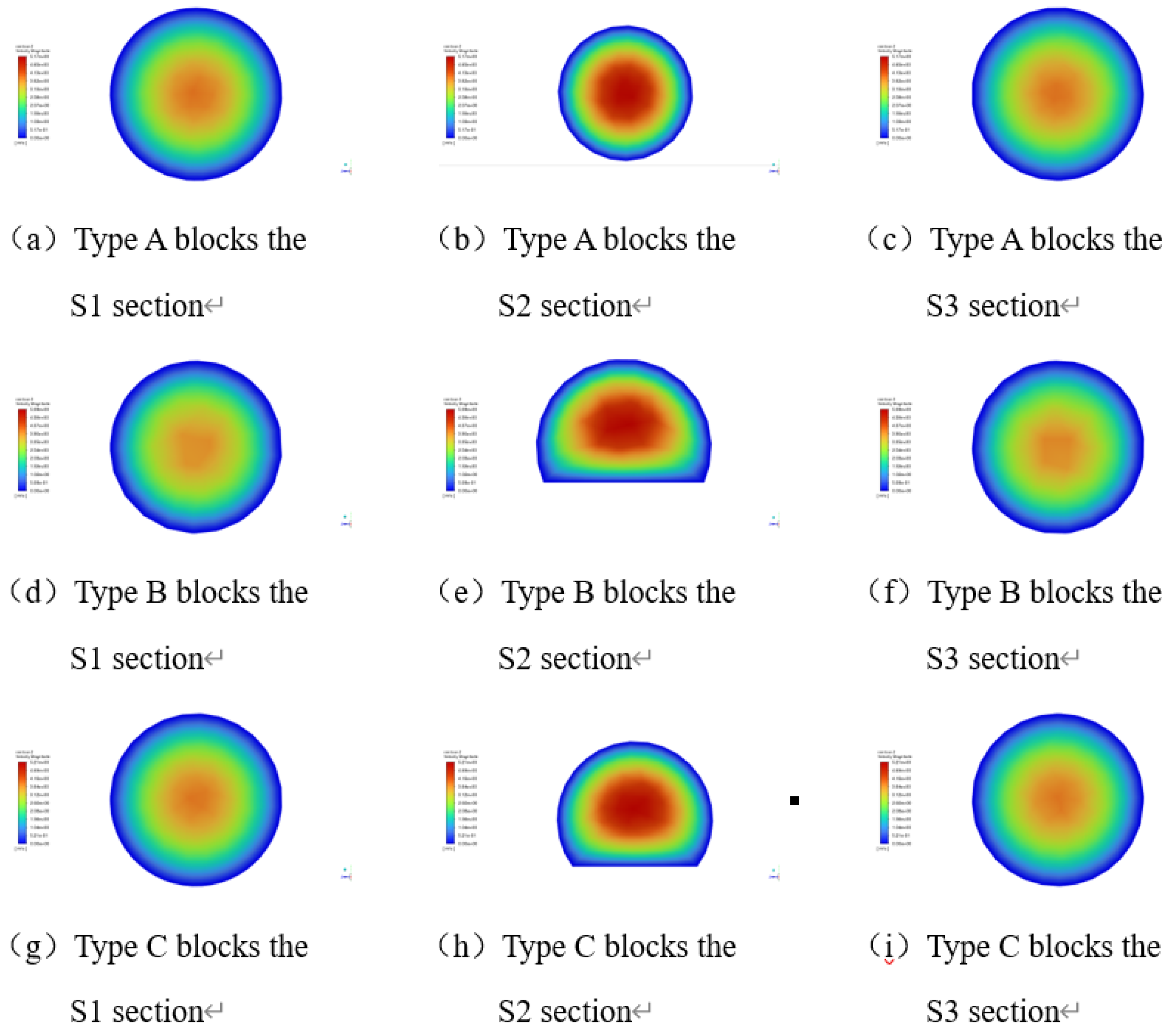
As seen in
Figure 16, the slurry transport inside the pipeline exhibits distinct laminar flow behavior for all three blockage shapes. During the pipeline transport of the filling slurry, the maximum slurry velocity consistently occurs at the center of the pipeline, forming a “flow core” where the velocity remains high. In contrast, the flow velocity at the top and bottom of the pipeline is slower. This phenomenon is due to friction between the slurry and the pipeline’s top and bottom surfaces, which creates resistance, causing the slurry’s velocity to remain highest in the center of the pipe, while the flow at the bottom and top is relatively slower.
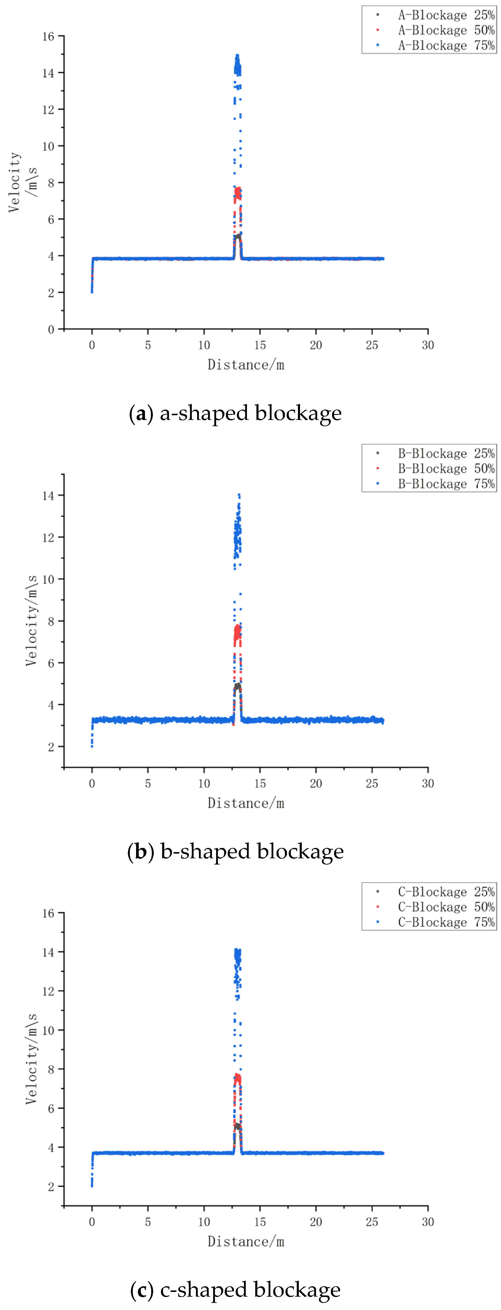
From
Figure 17, it can be observed that the flow velocity in the pipeline dramatically increases at the blockage location, reaching its maximum value within a short time. As the blockage degree increases, the velocity in the blocked region rises sharply, with the maximum flow velocity located at the center of the blockage. When the blockage degree exceeds 25%, the flow velocity in the blocked section is several times greater than that in the unblocked portion of the pipeline.
5. Conclusions
(1)Pressure and Velocity Gradients Near the Blockage: The presence of blockage results in significant pressure and velocity gradients near the blockage point. The larger the blockage, the greater the pressure gradient. When the blockage exceeds 50%, the pressure gradient changes, and there is a strong positive correlation between the pressure gradient and the characteristics of the blockage. Similarly, the velocity gradient increases with the blockage degree, and the relationship between the velocity gradient and the blockage characteristics is also positively correlated. Therefore, by detecting the pressure drop at the pipeline’s starting point, initial velocity, and the sharp changes in the pressure and velocity distribution curves, it is possible to detect and locate the blockage.
(2)Impact of Blockage Shape on Pressure: The effects of the three blockage shapes on the internal pressure of the pipeline are ranked as follows: sedimentation-type blockage has the greatest impact, followed by comprehensive-type blockage, and attachment-type blockage has the least impact. When the blockage degree is less than 50%, the changes in the pressure drop along the pipeline caused by the three blockage types are not significantly different. However, as the blockage degree increases, the pressure variations, particularly in sedimentation-type and comprehensive-type blockages, become more pronounced, with a larger fluctuation in the pressure along the pipeline. Among these, sedimentation-type blockages result in the most dramatic pressure changes. The formation of such blockages was analyzed in detail, and corresponding suggestions were proposed to address them.
(3)Flow Behavior and Safety: In all three blockage types, the flow of slurry in the pipeline is characterized by distinct laminar flow, with the maximum flow velocity occurring at the center of the pipeline, forming a “flow core.” The velocity at the top and bottom is lower due to friction with the pipeline surface. Moreover, the blockage shape significantly affects the flow velocity and pipeline safety. The stagnant flow region (dead zone) area for B-type and C-type blockages is larger than that for A-type blockages, underscoring the importance of timely blockage removal. To prevent blockages, it is recommended to use pipeline materials with smooth inner surfaces and low roughness.
Author Contributions
Conceptualization, L.Z. and Z.L.; methodology, L.Z. and C.L.; software, L.G.; validation, D.Z., J.C. and W.G.; data curation, C.M. and F.Q.; writing—original draft preparation, L.G. and D.Z.; writing—review and editing, L.Z. and D.Z.; visualization, D.Z. and Z.D. All authors have read and agreed to the published version of the manuscript.
Funding
This research received no external funding.
Institutional Review Board Statement
Not applicable.
Informed Consent Statement
Not applicable.
Data Availability Statement
The original contributions presented in the study are included in the article, further inquiries can be directed to the corresponding author.
Acknowledgments
We sincerely appreciate the time and effort of the editors and reviewers in evaluating the manuscript.
Conflicts of Interest
The authors declare that the research was conducted in the absence of any commercial or financial relationships that could be construed as a potential conflict of interest.
References
- Zhu, L.; Gu, W.Z.; Yuan, C.F.; et al. Application and Prospect of Coal Gangue Slurry Filling Technology. Coal Sci. Technol. 2024, 52, 93–104. [Google Scholar]
- Zhu, L.; Song, T.Q.; Gu, W.Z. Research and Application of Coal-Based Solid Waste Slurry Pipeline Filling Technology. Coal Technol. 2021, 40, 47–51. [Google Scholar]
- Lile, N.L.T.; Jaafar, M.H.M.; Roslan, M.R.; et al. Blockage Detection in Circular Pipe Using Vibration Analysis. Adv. Sci. Eng. Inf. Technol. 2012, 2, 54–57. [Google Scholar] [CrossRef]
- Kim, Y.; Simpson, A.R.; Lambert, M.F. The Effect of Orifices and Blockages on Unsteady Pipe Flows. World Environ. Water Resour. Congr. 2007, 157, 1–10. [Google Scholar]
- Adewumi, M.A.; Eltohami, E.; Solaja, A. Possible Detection of Multiple Blockages Using Transients. J. Energy Resour. Technol. 2003, 125, 154–158. [Google Scholar] [CrossRef]
- Zhao, L.A.; Xu, Z.L. Cause Analysis and Prevention Measures of Pipeline Blockage in Slurry Transportation. J. Liaoning Tech. Univ. Nat. Sci. Ed. 2009, 28, 10–12. [Google Scholar]
- Zhang, Q.L.; Wu, L.H.; Bian, J.W. Fault Tree Analysis of Filling Pipeline Blockage. Metall. Min. 2015, 44, 145–148. [Google Scholar]
- Han, X.J.; Li, X.S.; Dai, S.P.; et al. Cause Analysis of Pipeline Blockage Caused by Instantaneous High Flow Velocity of Filling Slurry. Nonferrous Metals (Mining Sect.) 2016, 68, 19–22. [Google Scholar]
- Liu, F.M. Numerical Simulation of Flow Characteristics in Long-Distance Slurry Pipelines. Coal Mine Mach. 2018, 39, 129–131. [Google Scholar]
- Wang, C.C.; Xu, J.L.; Xuan, D.Y. Research on the Blockage Mechanism of Ground Slurry Transport Pipeline Isolated by Overburden Grouting. Coal Sci. Technol. 2018, 43, 2703–2708. [Google Scholar]
- Song, B.K. Study on Pipeline Blockage Detection Method Based on Pressure Wave. Ph.D. Thesis, Yangtze University, Wuhan, China, 2019. [Google Scholar]
- Wang, J.L.; Xiong, Y.H.; Zhang, Y.Q.; et al. CFD Simulation of Drainage Pipeline Blockage. Sci. Technol. Eng. 2023, 23, 6607–6613. [Google Scholar]
- Han, G.J. Fundamentals and Applications of Fluid Mechanics; Mechanical Industry Press: Beijing, China, 2012. [Google Scholar]
- Gan, D.Q.; Gao, F.; Chen, C.; Liu, A.X.; Zhang, Y.P. Numerical Simulation of High-Concentration Tailings Slurry Pipeline Transportation. Metall. Min. 2014, 10, 138–141. [Google Scholar]
- Shi, H.W.; Huang, J.R.; Qiao, D.P.; Teng, G.L.; Wang, B. ANSYS Fluent-Based Simulation Study on Ultra-Deep Well Long-Distance Paste Filling Pipeline. Nonferrous Metals (Mining Sect.) 2020, 72, 5–12. [Google Scholar]
- Wang, X.M.; Ding, D.Q.; Wu, Y.B.; Zhang, Q.L.; Lu, Y.Z. Numerical Simulation and Analysis of Paste Filling Pipeline Transportation. China Min. 2006, 57–59, 66. [Google Scholar]
- Chen, X.N. CFD-Based Flow Pattern Analysis and Resistance Loss Model Study for Solid-Liquid Two-Phase Flow. Ph.D. Thesis, Kunming University of Science and Technology, Kunming, China, 2017. [Google Scholar]
- Qiu, Y.Q. Analysis of Two Resistance Loss Calculation Methods in Slurry Pipeline Transportation. J. Guizhou Univ. Ind. Sci. Technol. 1999, 5, 457–459. [Google Scholar]
- Lu, H.; Yin, J.; Yuan, Y.X.; et al. Resistance Mechanism and Drag Reduction Technology for Slurry Pipeline Transportation. J. Qingdao Univ. Technol. 2016, 32, 90–95. [Google Scholar]
- Fei, X.J. Hydraulics of Slurry and Granular Material Transport; Tsinghua University Press: Beijing, China, 1994; pp. 390–392. [Google Scholar]
- Li, T. Research on Hydraulic Transport Power Characteristics of Slurry Pipeline. Ph.D. Thesis, Wuhan University of Technology, Wuhan, China, 2013. [Google Scholar]
|
Disclaimer/Publisher’s Note: The statements, opinions and data contained in all publications are solely those of the individual author(s) and contributor(s) and not of MDPI and/or the editor(s). MDPI and/or the editor(s) disclaim responsibility for any injury to people or property resulting from any ideas, methods, instructions or products referred to in the content. |
© 2024 by the authors. Licensee MDPI, Basel, Switzerland. This article is an open access article distributed under the terms and conditions of the Creative Commons Attribution (CC BY) license (http://creativecommons.org/licenses/by/4.0/).