
Submitted:
15 December 2024
Posted:
17 December 2024
Read the latest preprint version here
Abstract
The primary challenge in robotic navigation lies in enabling robots to adapt effectively to new, unseen environments. Addressing this gap, this paper enhances the Twin Delayed Deep Deterministic Policy Gradient (TD3) model’s adaptability by introducing randomized start and goal points. This approach aims to overcome the limitations of fixed goal points used in prior research, allowing the robot to navigate more effectively through unpredictable scenarios. This proposed extension was evaluated in unseen environments to validate the enhanced adaptability and performance of the TD3 model. The experimental results highlight improved flexibility and robustness in the robot’s navigation capabilities, demonstrating the model’s ability to generalize effectively to unseen environments. In addition, this paper presents an overview of the TD3 algorithm’s architecture and principles, with an emphasis on key components like the actor and critic networks, their updates, and mitigation of overestimation bias. The goal is to provide a clearer understanding of how the TD3 framework is adapted and utilized in this study to achieve improved performance.
Keywords:
reinforcement learning
; TD3
; SAC
; Jackal robot
; robust navigation
; transferability
1. Introduction
Reinforcement learning (RL) has become a powerful tool in developing adaptive control policies for autonomous robots navigating complex environments [19]. As autonomous systems, particularly mobile robots, are deployed in dynamic and unpredictable real-world settings, robust navigation strategies are crucial. This challenge is especially relevant for skid-steered robots, widely known for their durability and versatility in various robotic applications [2]. Despite their potential, enabling these robots to navigate efficiently and safely through diverse and unseen environments remains a significant research challenge.
The choice of RL algorithm is critical in developing navigation policies that are both efficient and adaptable [1]. Twin Delayed Deep Deterministic Policy Gradient (TD3), introduced by Fujimoto et al. at NeurIPS [3], is a state-of-the-art RL algorithm designed to address overestimation bias and improve policy stability in continuous control tasks. TD3 improves upon earlier methods, such as Deep Deterministic Policy Gradient (DDPG) [11], through dual critic networks and delayed updates to the policy, which help mitigate overestimation errors and improve the stability of learned policies. Additionally, TD3 leverages a noise signal to promote effective exploration of the action space, preventing premature convergence to suboptimal solutions.
Recent Deep Reinforcement Learning (DRL) methods[6], such as DreamerV2 [7], and Multi-view Prompting (MvP) [22], have demonstrated significant advancements, methods like TD3, Soft Actor-Critic (SAC) [8], and Proximal Policy Optimization (PPO) [9] have gained wide adoption for their compatibility with various data science and machine learning tools. Older techniques, such as DQN [10], and DDPG, have seen reduced usage due to the superior performance of newer methods like TD3. Empirical results from benchmarks, such as the OpenAI Gym environments, demonstrate that TD3 outperforms several contemporary algorithms, including DDPG, in various control tasks [19].
Recent studies by authors who have successfully made physical deployments of DRL-based navigation systems highlight the strengths and innovative approaches in this field.
Xu et al. [4,19,24] applied DDPG, SAC, and TD3 in a range of static and dynamic environments with diverse difficulty levels. Their work involved 300 static environments, each consisting of 4.5m x 4.5m fields with obstacles placed on three edges of a square [24]. They also used dynamic-box environments featuring 13.5m x 13.5m fields with randomly moving obstacles of varying shapes, sizes, and velocities, as well as dynamic-wall environments comprising 4.5m x 4.5m fields with parallel walls that move in opposite directions at various random locations. These dynamic-wall environments required long-term decision-making to navigate the moving obstacles successfully. Additionally, dynamic objects were introduced that moved randomly with different speeds, shapes, and sizes, further adding complexity [24]. They achieved success rates of 60-74%, with the highest performance observed in static environments. A key strength of their approach was the use of distributed training pipelines, which significantly reduced training time by running multiple model instances in parallel, optimizing the use of computational resources such as CPUs and GPUs.
Anas et al. [5,13] focused on TD3 for training and testing navigation in a 2m x 2m indoor space with 14 obstacles. Despite achieving a 100% success rate in simulation, challenges were faced during real-world deployment involving manually controlled obstacles. This work introduced Collision Probability (CP) as a metric for perceived risk, adding an important dimension to risk assessment in navigation tasks.
Cimurs et al. [12,23] deployed TD3 in environments where obstacles were placed randomly at the start of each episode, combining global navigation for waypoint selection with local TD3-based navigation to guide the robot through obstacles. This strategy enabled effective goal-reaching and obstacle avoidance, demonstrating the strength of integrating global navigation strategies with local reinforcement learning-based navigation.
Akmandor et al.[14,15] employed hierarchical training using PPO, progressing from simple to more complex static and dynamic obstacle environments. The integration of heuristic global navigation with PPO-based local navigation allowed the robot to effectively learn strategies such as overtaking agents moving towards it and avoiding agents crossing its path, contributing to higher success rates, particularly in dynamic conditions.
Roth et al. [17,18] also used PPO for real-world deployment with the Clearpath Jackal robot in environments similar to those used in simulation, adjusted for real-world conditions. This work uniquely integrated Explainable AI (XAI) techniques by transforming DRL policies into decision trees, enhancing the interpretability and modifiability of navigation decisions, which is especially useful for real-world deployment scenarios.
These studies, while advancing DRL-based navigation, exhibit common limitations, particularly in the ability of models to adapt effectively to completely unseen and dynamic environments. The reliance on fixed start and goal points or controlled environments restricts the robot’s capacity to generalize across different navigation scenarios, which remains a key challenge in RL-based robotics.
The primary contribution of this work lies in extending the TD3 algorithm to improve generalization in robot navigation. Traditional RL-based models tend to excel in environments similar to those used during training but often struggle in unfamiliar settings. To address this, our approach introduces randomized start and goal points, allowing the Jackal robot to develop more flexible and adaptive navigation strategies. By enhancing the robot’s ability to navigate in dynamic, unseen environments, this research aims to bridge the gap between simulation-based training and real-world deployment and overcome the generalization challenges identified in previous studies.
The rest of this paper is arranged as follows, Section 3 provides a background of the TD3 algorithm and key concepts related to its robustness in robot navigation tasks. Section 2 discusses the research gaps and motivation for extending existing work, particularly focusing on the limitations of current end-to-end deep reinforcement learning (DRL) deployments. Section 4 outlines the methodology and experimental setup used to assess the extended TD3 model’s performance. Section 5 outlines the experimental design and the evaluation metrics used to compare the performance of the two TD3 models. Section 6 presents the training results and comparative analysis of our extended TD3 model with non-extended setups. Finally, Section 7 evaluates the model’s ability to generalize across unseen environments, and Section 8 concludes the paper with key findings and recommendations for future work in DRL-based robot navigation.
2. Research Gaps and Motivation for Extending Existing Work
Despite recent advancements in deep reinforcement learning (DRL) for robot navigation, significant challenges remain. Many approaches, though effective in controlled scenarios, struggle to generalize to diverse and unseen environments. A common issue is the reliance on fixed start and goal points during training, limiting adaptability in dynamic real-world conditions.
For example, Xu et al. [4,19] applied TD3, DDPG, and SAC in both static and dynamic environments. Despite using numerous scenarios, the fixed start and goal configurations hindered generalization, resulting in success rates between 60-74%, with better performance in static environments. This suggests limited adaptability to unexpected goal points.
This limitation is not unique to Xu et al.’s work. Many researchers have developed DRL models that excel in training environments but struggle in unseen settings. Cimurs et al. [12,23] achieved impressive simulation results but faced challenges in real-world deployment involving manually controlled obstacles, highlighting the gap between simulation and practical application.
Similarly, Akmandor et al. [14,15] used a combination of global and local navigation strategies, yielding promising results for obstacle avoidance. However, like other studies, their approach did not fully explore variability in start and goal points, limiting robust generalization.
To address these research gaps, this work extends Xu et al.’s approach by enhancing the exploration capabilities of the TD3 model. The proposed extension introduces randomly generated start and goal points, as well as varying robot orientations during training. These modifications significantly improve the model’s learning capacity by allowing the robot to explore a wider range of situations, increasing its adaptability to dynamic and unpredictable environments.
By building on Xu et al.’s distributed rollout framework, this study aims to bridge the gap between controlled, simulation-based training and practical, real-world applications. The proposed enhancements ensure that the robot can learn in diverse and dynamic scenarios, making it more robust when facing unexpected changes in real-world navigation tasks. This contribution advances the state of the art in DRL-based robot navigation by developing a more adaptable and scalable solution for real-world scenarios.
3. Background
3.1. TD3 Architecture and Principles
The architecture of TD3 consists of several key components as defined by Scott Fujimoto et al. [3]: the actor network, two critic networks, and their corresponding target networks (see Figure 1). The following is a detailed explanation of each component:
- Policy Network (Actor Network): The actor network, denoted as , is responsible for selecting actions given the current state. It approximates the policy function and is parameterized by . The actor network outputs the action that the agent should take in a given state to maximize the expected return.
- Critic Networks ( and ): TD3 employs two critic networks, and , to estimate the Q-values for state-action pairs . Each network outputs a scalar value that represents the expected return for a specific state-action pair. The use of two critics helps to reduce overestimation bias, which can occur when function approximation is used in reinforcement learning. By employing double Q-learning, TD3 ensures more accurate value estimates, enhancing the stability of policy updates.
- Critic Target Networks: The critic target networks, and , are delayed versions of the primary critic networks and are updated at a slower rate. These target networks provide stable Q-value targets for the critic updates, which helps to reduce variance and prevents divergence during training. By maintaining more conservative Q-value estimates, the critic target networks further mitigate the overestimation bias found in reinforcement learning models.
- Actor Target Network: The actor target network, , is a delayed copy of the actor network and is essential for generating stable action targets for the critic updates. The actor target network changes gradually over time, ensuring that the target actions used in critic updates are consistent and stable. This stability is critical for reducing the variance in the Q-value targets provided by the critic target networks, leading to more reliable and stable training of the critics. The actor target network’s slow updates help in maintaining a steady learning process and improve the overall performance of the TD3 algorithm by preventing rapid and unstable policy changes.
3.2. Policy Network Updates
To update the policy network (actor) in TD3, the policy gradient must be calculated. The deterministic policy gradient theorem forms the theoretical basis for adjusting the policy parameters. The aim is to maximize the expected return , defined as:
where:
- represents the action selected by the policy given state s.
- denotes the critic (value function) estimating the expected return of taking action a in state s and following policy .
- denotes the state distribution under policy .
3.2.1. Policy Gradient Computation
The deterministic policy gradient theorem states that the gradient of the expected return with respect to the policy parameters is given by:
This expression is composed of two terms: 1. Gradient of the Q-Value with Respect to the Action:
This term captures the change in the Q-value relative to the action, evaluated at the action proposed by the current policy . 2. Policy Gradient with Respect to policy networks Parameters:
This term captures how the selected action changes with respect to changes in the policy parameters .
3.2.2. Policy Gradient and Parameter Update
The policy gradient and the parameter update rule are defined as follows:
where:
- represents the learning rate used for updating the policy network.
- denotes the gradient of the Q-value function with respect to the action, evaluated at the action chosen by the current policy.
- represents the policy gradient calculated with respect to the parameters of the policy.
- N indicates the size of the mini-batch used during the update process.
3.3. Q Networks Updates
3.3.1. Overestimation Bias in Q-learning and Mitigation Approaches
In standard Q-learning, Q-learning, the Q-value update depends on the highest Q-value for the next state. However, inaccuracies in function approximation can cause this maximum to be overestimated, creating an upward bias in the Q-values over time and potentially leading the algorithm to select suboptimal actions. Double Q-learning addresses this bias by separating the action selection process from the estimation of the target Q-value, maintaining two separate Q-value estimates, and using one for selecting actions and the other for evaluation. Clipped Double Q-learning in TD3 extends this approach by using two Q-networks ( and ) and calculating the target value as the minimum of the two Q-value estimates, ensuring the target value is less likely to be overestimated because the minimum of two estimates is less prone to upward bias than a single estimate.
3.3.2. TD3 Algorithm Q-Network Updates
The TD3 algorithm maintains two Q-networks ( and ) and their corresponding target networks ( and ). The updates to these Q-networks aim to minimize overestimation bias by using the minimum of the two target Q-values. The process involves several steps: sampling a mini-batch of N transitions from the replay buffer, computing the target action using the target actor network with added noise for regularization , and calculating the target Q-values using the target critics. Finally, the target value y is computed as the minimum of the two Q-values:
The Q-networks are then updated by minimizing the mean squared error between their predicted Q-values and this target value.
3.3.3. Q Networks Parameters Updates
Update each Q-network by minimizing the mean squared error (MSE) between the predicted Q-values and the target value y:
For :
For :
where:
- and are the parameters of the Q-networks and , respectively.
- N denotes the mini-batch size.
- indicates the j-th transition in the mini-batch.
- and are the predicted Q-values from the Q-networks for the j-th state-action pair.
- is the target value for the j-th transition, as described above.
Note: In the TD3 algorithm, the actor (policy) network is updated with a delay compared to the critic (Q) networks. Specifically, the actor-network is updated every d steps, while the critic networks are updated at every time step. This delay helps to stabilize training by ensuring that the value estimates provided by the critic networks are accurate before the policy is updated. Frequent updates to the actor-network can lead to instability and poor performance due to the propagation of errors in the value estimates. By updating the actor-network less frequently, TD3 reduces the likelihood of such issues and promotes more stable and reliable learning.
3.3.4. Target Networks Update
The target networks in the TD3 algorithm are used to provide stable target values for the critic updates. The target networks are updated using a soft update mechanism, where the parameters of the target networks are slowly updated towards the parameters of the current networks. This is done using a factor , which determines the rate of the update.
- Initialize target networks to match the parameters of the current networks:
- Soft update the target Q-networks after every d steps:
- Soft update the target actor network after every d steps:
4. Methodology and Experimental Setup
The research methodology operates within a Singularity container, integrating the Noetic ROS system framework with a simulation of the Jackal robot and a custom OpenAI Gym environment. These components work together with deep reinforcement learning (RL), initialized using the PyTorch library, to train the robot for navigation tasks.
All simulations are conducted in the Gazebo simulator, specifically within a custom motion control environment, called the MotionControlContinuousLaser environment. This environment is designed for the Jackal robot and provides a continuous action space consisting of linear and angular velocities, enabling smooth robot movement. It also processes the 720-dimensional laser scan data, incorporating it into the observation space, allowing the agent to access essential sensory information for decision-making. By integrating both motion control and laser scan data processing, the environment offers a challenging scenario for evaluating reinforcement learning algorithms in a realistic context.
The training data is collected through interactions in the simulated environments and saved locally. The data is stored in a replay buffer, allowing randomized sampling during the training process. The model’s parameters are updated continuously, and new policies are saved locally until the model converges.
4.1. Jackal Robot Dynamics and Sensors
The Jackal robot is equipped with two primary sensors directly connected to the reinforcement learning (DRL) algorithm and the robot’s control system:
- Laser Sensor: The LiDAR sensor provides essential data for navigation by scanning the environment and detecting obstacles. It generates a 720-dimensional laser scan, which is directly used by the DRL algorithm to inform the robot’s decision-making process. This data enables the robot to avoid collisions and select efficient paths to reach its goal. In the Gazebo simulation, the LiDAR sensor replicates real-world sensor dynamics, ensuring that the robot can adapt to complex environments during training.
- Velocity Sensor: The velocity sensor monitors the robot’s movement by tracking the linear and angular velocities issued by the DRL node. These commands control the robot’s speed, ensuring that the actual movement matches the intended commands. This feedback helps maintain stable movement and highlights any deviations, such as low velocity, that may affect navigation performance.
4.2. Training and Evaluation Scenarios
Two types of environments were used for training evaluation:
4.2.1. Static Box Environments
: In line with previous work [4], the static box environment measuring 4.5m x 4.5m was used for training. This environment consists of stationary obstacles arranged in various patterns, providing a controlled setting to assess the robot’s navigation performance under static conditions. Figure 2 shows the layout of the static box environment as originally used in Xu’s study [24].
4.2.2. Custom Static Environments
: These custom environments consist of 16 unique scenarios, each with distinct designs and varying object positions, creating a diverse range of challenges for the robot. Unlike the original 4.5m x 4.5m static boxes, which limited flexibility due to their small size, these environments are expanded to 16m x 16m, providing ample space for randomization of start and goal points in each episode. This increased area not only facilitates better exploration but also ensures more robust generalization by exposing the robot to a wider variety of paths and obstacles. Each scenario is specifically tailored with unique layouts, different difficulty levels, and diverse obstacle configurations, all designed to enhance the robot’s adaptability, robustness, and overall navigation performance in complex settings. Figure 3 illustrates several examples of these custom environments.
5. Experimental Comparison of TD3 Models
The goal of this experiment is to compare the performance of our improved TD3 model, trained using 16 custom static environments defined in the previous section (Section 4), with the baseline model trained by Xu et al. [4] on 300 static environments from the original setup. By contrasting these two models, we aim to determine the impact of environment diversity and training methodology on overall performance.
5.1. Training and Evaluation Metrics
For the evaluation of our improved TD3 model, a comprehensive set of performance metrics will be used to provide a thorough analysis of the model’s behavior in unseen environments. The key metrics include:
- Success Rate: The percentage of episodes where the robot successfully reaches the goal without collisions.
- Collision Rate: The percentage of episodes where the robot collides with obstacles.
- Episode Length: The average duration (in terms of steps) taken by the robot to complete a task.
- Average Return: The cumulative reward earned by the robot over an episode, averaged over all episodes, to evaluate the learning efficiency of the algorithm.
- Time-Averaged Number of Steps: The average number of steps the robot takes to complete each episode, providing insight into the efficiency of the navigation strategy.
- Total Distance Traveled: This metric, calculated during the test phase, measures the total distance (in meters) the robot travels to complete a path. It provides an additional layer of analysis by assessing the efficiency of the robot’s movements in terms of path length.
6. Training Results and Comparison
This section compares the performance of the extended model (blue plot) and the non-extended model (orange plot), focusing on success rate, collision rate, and average return.
6.1. Success Rate Comparison
As shown in Figure 4, the extended model achieved a success rate of 95%, converging before 2 million steps, while the non-extended model reached 70% after 3 million steps. This indicates the extended model’s faster learning speed and higher efficiency due to the randomization of start and goal points.
6.2. Collision Rate Analysis
Figure 5 shows that the extended model had a final collision rate of 4%, compared to 24% for the non-extended model. Both models saw improvements early in training, but the non-extended model’s collision rate increased again after 3.5 million steps, suggesting overtraining. The extended model maintained a more consistent collision reduction.
6.3. Average Return and Learning Efficiency
As shown in Figure 6, the extended model consistently achieved higher average returns throughout the training process, indicating better adaptability and performance across diverse environments. This improvement can be attributed to the randomization of start and goal points, which allowed the robot to explore a wider variety of scenarios and develop more general navigation strategies.
6.4. Training Efficiency and Convergence
The extended model demonstrated faster convergence and learning efficiency, reaching optimal performance with fewer training steps. The randomization of start and goal points enabled the extended model to explore more diverse environments, resulting in higher success rates. In contrast, the non-extended model, which was trained with fixed start and goal points, showed slower progress and lower success rates. Additionally, some of the environments used by the non-extended model were extremely narrow, which may have limited the robot’s ability to achieve a higher success rate.
7. Transfer to Test Environments Using TD3 and Global Path Planning
To evaluate the generalizability of the extended model, transfer tests were conducted using the Competition Package [20]. The environment used for this evaluation resembles a maze, with long walls that make it challenging for the robot to determine the correct direction toward the goal. Both the extended model and the non-extended model were not trained in such maze-like scenarios, increasing the difficulty of navigating this environment. The specific environment used here is Race World [21].
In these tests, the move_base package [25] was utilized to provide a global path planning strategy, while the main navigation was handled using the TD3 algorithm. The move_base package was responsible for generating a global path from the start to the goal, providing a reference path for the robot. The TD3-based controller then followed this global path, adapting locally in real time to avoid obstacles and navigate effectively. This hybrid strategy allowed the robot to utilize the global path for overall guidance while leveraging the adaptability of the TD3-based navigation to handle local dynamic challenges.
7.1. Evaluation Results
Table 1 and Table 2 present the evaluation results for the extended and non-extended models, respectively. These tables provide key metrics, including the total distance traveled, the number of collisions, and the success status for each of the 10 test paths. The test paths used for evaluation are detailed in Figure 7. The results highlight the superior performance of the extended model, which consistently achieved a higher success rate and fewer collisions compared to the non-extended model. Additionally, the extended model demonstrated more efficient navigation by achieving closer-to-optimal distances on most paths. In contrast, the non-extended model struggled significantly on certain complex paths, often leading to failed navigation attempts or a higher number of collisions.
7.2. Analysis of Results
Success Rate and Distance Traveled: The extended model consistently outperformed the non-extended model in terms of success rate and total distance traveled. For instance, in Path 1, the extended model completed the navigation in 18.72 meters with no collisions, achieving a success metric of 100%. In contrast, the non-extended model failed, covering a distance of 33.53 meters with 4 collisions, resulting in a navigation metric of 0%. This highlights the extended model’s ability to stay closer to the optimal path, demonstrating superior generalization and efficient navigation without deviations. The non-extended model, however, faced significant challenges adapting to these scenarios.
Collision Rate and Penalties: The extended model exhibited a considerably lower collision rate across all paths, with either zero or minimal collisions, whereas the non-extended model encountered multiple collisions in most paths. For example, in Path 4, the extended model recorded 4 collisions and failed, achieving a metric of 0%, while the non-extended model also failed with 3 collisions and an even higher distance penalty, resulting in similarly low performance metrics. In contrast, the extended model achieved 100% on paths where collisions were avoided, showing superior collision avoidance and efficient navigation.
Time and Distance Efficiency: The extended model demonstrated better time and distance efficiency in all paths. For instance, in Path 5, the extended model completed the navigation in 9.26 seconds, covering 15.51 meters, while the non-extended model took 42.20 seconds, covering a less optimal path of 32.09 meters. This efficiency showcases the extended model’s ability to make precise navigation decisions in real time, completing tasks faster while adhering closely to the optimal route.
Generalization and Adaptability: The extended model’s superior generalization capability to navigate unseen environments was evident in its successful completion of complex paths with minimal collisions and reduced distances, as shown in Table 1 and Table 2. In Figure 8 and Figure 9, the same paths taken by both models in Path 1 and Path 2 highlight this distinction. The extended model’s trajectory is smooth and efficient, whereas the non-extended model displayed significant deviations and struggled to adapt to the scenario.
Challenges with Non-Straightforward Goals: The non-extended model showed significant difficulty when the goal was not directly aligned with the start point, reflecting a limitation in its ability to navigate complex paths. Trained with fixed start and goal points, the non-extended model primarily learned straightforward navigation, which proved insufficient in the test environments featuring complex turns and long walls (e.g., Paths 2 and 8). In Path 2, for example, the extended model navigated efficiently with a success metric of 57.60%, completing the path without timing out, whereas the non-extended model timed out after traveling an inefficient distance of 41.97 meters.
The extended model’s ability to navigate non-straightforward paths is attributed to its training with randomized start and goal points, which fostered a broader exploration capability and adaptability to dynamic environments, ultimately resulting in higher success rates and reduced penalties during testing.
7.3. Custom Navigation Performance Assessment Score Comparison
Evaluating navigation performance in real-world scenarios requires a metric that accounts for more than binary success or failure. The proposed custom navigation performance score metric better reflects real-world robot behavior by grading performance on a scale from 0% to 100%. This metric evaluates the robot’s efficiency and safety in reaching its goal by considering three key factors: distance traveled, time taken, and the number of collisions. Unlike traditional binary metrics that label navigation attempts as either successful or failed, this score allows for partial successes, acknowledging scenarios where the robot reaches the goal despite minor inefficiencies or collisions. Such graded scoring is critical for realistic evaluations, as in practical applications, minor collisions or suboptimal paths may still be acceptable. By integrating these penalties, the custom metric provides a more nuanced evaluation of robot performance, reflecting real-world decision-making scenarios where navigation is judged not only by reaching the goal but also by the efficiency and safety of the path taken. This approach complements traditional success metrics by offering deeper insights into the robot’s adaptability and robustness. Each test starts with a base score of 100%, with penalties applied based on performance deviations:
where
Each penalty term is defined as follows:
Distance Penalty (): Applied if the path length exceeds twice the optimal distance. The distance penalty is proportional to the excess distance traveled over twice the optimal distance and is capped at a maximum of 33%. The formula used is:
where max_allowed_distance is four times the optimal distance. If this calculated penalty exceeds 33%, it is capped at 33%.
Time Penalty (): Applied if the actual navigation time exceeds 40 seconds. This penalty increases with time beyond 40 seconds and is capped at 33%. The calculation is:
If this calculated penalty exceeds 33%, it is capped at 33%.
Collision Penalty (): Applied based on the number of collisions, with a penalty of 11% per collision. This penalty is capped at a maximum of 3 collisions, leading to a maximum collision penalty of 33%:
If this calculated penalty exceeds 33%, it is capped at 33%.
In this scoring system, a score of 0% is assigned if the robot fails to reach the goal, exceeds four times the optimal distance, or incurs more than 3 collisions. Table 3 and Table 4 show that the extended model consistently achieved higher scores, demonstrating more efficient navigation, fewer collisions, and superior adaptability. This is further illustrated in Figure 8, Figure 8, Figure 8, Figure 9, Figure 9, and Figure 9, which compare the trajectories of the extended and non-extended models for Paths 1 and 2 using RViz visualization. The figures highlight how the extended model navigates more efficiently with fewer collisions and smoother trajectories, while the non-extended model struggles with significant deviations and higher collision rates during navigation.
8. Conclusion and Recommendations
Our evaluation of both extended and non-extended environments reveals a significant research gap in robot navigation using deep reinforcement learning (DRL). While models tend to perform well in familiar environments, they often struggle to generalize to unseen environments, highlighting the need to improve the adaptability and robustness of DRL-based navigation systems.
The proposed extension specifically targets this research gap, which has been insufficiently addressed in previous work. The key insight from this study is that robust generalization is better achieved by training with varied and dynamic start and goal points rather than increasing the number of training scenarios, as done in the non-extended model. This diversity allows the robot to adapt more effectively to unforeseen environments, a perspective not often emphasized in recent studies.
In terms of performance, the non-extended model demonstrates an advantage in navigating extremely narrow environments, likely due to specific training for such conditions. However, it struggles with unpredictable goal points, even in simpler environments. In contrast, the extended model, which emphasizes start and goal diversity, adapts well to unpredictable navigation tasks but may face challenges in extremely narrow environments. This highlights the complementary strengths of both approaches. We recommend that future work combines the strengths of both models. Training should include diverse start and goal points, as in this extension, while also incorporating narrow and extremely narrow environments to enhance performance in highly constrained spaces.
Acknowledgments
The authors express their sincere gratitude to the SCUDO Office at Politecnico di Torino for their vital support and assistance throughout this research. Special thanks are extended to REPLY Concepts company for their valuable contributions and collaboration. The authors also acknowledge the Department of DAUIN at Politecnico di Torino and the team at PIC4SeR Interdepartmental Centre for Service Robotics - www.pic4ser.polito.it for their continued support and cooperation. Further appreciation is given to the Electrical and Computer Engineering Department of the University of Coimbra and the Institute for Systems and Robotics (ISR-UC) for their collaboration and assistance. This work was financially supported by the AM2R project, a Mobilizing Agenda for business innovation in the Two Wheels sector, funded by the PRR - Recovery and Resilience Plan and the Next Generation EU Funds under reference C644866475-00000012 | 7253. This paper is the result of a collaborative effort between Politecnico di Torino and the University of Coimbra.
References
- R. S. Sutton and A. G. Barto, Reinforcement Learning: An Introduction, 2nd ed. Cambridge, MA, USA: MIT Press, 2018.
- Y. Chen, C. Y. Chen, C. Rastogi, and W. R. Norris, "A CNN Based Vision-Proprioception Fusion Method for Robust UGV Terrain Classification," IEEE Robotics Autom. Lett., vol. 6, no. 4, pp. 7965–7972, 2021. [Online]. Available. [CrossRef]
- S. Fujimoto, H. S. Fujimoto, H. van Hoof, and D. Meger, "Addressing Function Approximation Error in Actor-Critic Methods," in Proceedings of the 35th International Conference on Machine Learning, ICML 2018, Stockholmsmässan, Stockholm, Sweden, vol. 80, pp. 1582–1591, 2018. [Online]. Available: http://proceedings.mlr.press/v80/fujimoto18a.html.
- F. Daffan, "ros_jackal," GitHub repository, 2021. [Online]. Available: https://github.com/Daffan/ros_jackal. [Accessed, 2024.
- H. Anas, O. W. H. Anas, O. W. Hong, and O. A. Malik, "Deep Reinforcement Learning-Based Mapless Crowd Navigation with Perceived Risk of the Moving Crowd for Mobile Robots," in 2nd Workshop on Social Robot Navigation, IEEE/RSJ International Conference on Intelligent Robots and Systems (IROS), 2023.
- M. Lapan, Deep Reinforcement Learning Hands-On: Apply Modern RL Methods, with Deep Q-networks, Value Iteration, Policy Gradients, TRPO, AlphaGo Zero and More, Packt Publishing, 2018. [Accessed: 24]. 20 October.
- D. Hafner, T. P. D. Hafner, T. P. Lillicrap, M. Norouzi, and J. Ba, "Mastering Atari with Discrete World Models," in Proceedings of the International Conference on Learning Representations (ICLR), 2021.
- T. Haarnoja, A. T. Haarnoja, A. Zhou, P. Abbeel, and S. Levine, "Soft Actor-Critic: Off-Policy Maximum Entropy Deep Reinforcement Learning with a Stochastic Actor," CoRR, vol. abs/1801.01290, 2018.
- J. Schulman, F. J. Schulman, F. Wolski, P. Dhariwal, A. Radford, and O. Klimov, "Proximal Policy Optimization Algorithms," CoRR, vol. abs/1707.06347, 2017. [Online].
- V. Mnih, K. V. Mnih, K. Kavukcuoglu, D. Silver, A. Graves, I. Antonoglou, D. Wierstra, and M. Riedmiller, "Playing Atari with Deep Reinforcement Learning," in Proceedings of the Annual Conference on Neural Information Processing Systems (NeurIPS), 2015. [Online].
- T. P. Lillicrap, J. J. T. P. Lillicrap, J. J. Hunt, A. Pritzel, N. Heess, T. Erez, Y. Tassa, D. Silver, and D. Wierstra, "Continuous Control with Deep Reinforcement Learning," in Proceedings of the International Conference on Learning Representations (ICLR), 2016.
- R. Cimurs, "DRL-robot-navigation," GitHub repository, 2024. [Online]. Available: https://github.com/reiniscimurs/DRL-robot-navigation. [Accessed: Sep. 2024.
- Zerosansan, "TD3, DDPG, SAC, DQN, Q-Learning, SARSA Mobile Robot Navigation," GitHub repository, 2024. [Online]. Available: https://github.com/zerosansan/td3_ddpg_sac_dqn_qlearning_sarsa_mobile_robot_navigation. [Accessed: Sep. 2024.
- N. U. Akmandor, H. Li, G. Lvov, E. Dusel, and T. Padır, "Deep Reinforcement Learning Based Robot Navigation in Dynamic Environments using Occupancy Values of Motion Primitives," in 2022 IEEE/RSJ International Conference on Intelligent Robots and Systems (IROS), Kyoto, Japan, 2022, pp. 9982133.
- N. U. Akmandor and E. Dusel, "Tentabot: Deep Reinforcement Learning-based Navigation," GitHub repository, 2022. [Online]. Available: https://github.com/RIVeR-Lab/tentabot/tree/master. [Accessed: Sep. 2024.
- Z. Wang, J. Z. Wang, J. Zhang, H. Yin, B. Yuan, and D. Manocha, "Dynamic Graph Learning for Efficient Exploration in Unknown Environments," IEEE Robotics and Automation Letters, vol. 7, no. 1, pp. 233-240, 2022. [Online]. Available. [CrossRef]
- A. M. Roth, "JackalCrowdEnv," GitHub repository, 2019. [Online]. Available: https://github.com/AMR-/JackalCrowdEnv. [Accessed, 2024.
- A. M. Roth, J. A. M. Roth, J. Liang, and D. Manocha, "XAI-N: Sensor-based Robot Navigation using Expert Policies and Decision Trees," in Proceedings of the IEEE/RSJ International Conference on Intelligent Robots and Systems (IROS), 2021.
- Z. Xu, B. Z. Xu, B. Liu, X. Xiao, A. Nair, and P. Stone, "Benchmarking Reinforcement Learning Techniques for Autonomous Navigation," in Proceedings of the IEEE International Conference on Robotics and Automation (ICRA), 2023, pp. 9224–9230.
- F. Daffan, "ROS Jackal: Competition Package," GitHub repository, 2023. [Online]. Available: https://github.com/Daffan/ros_jackal/tree/competition. ,: [Accessed, 22 October 2024.
- Clearpath Robotics, "Simulating Jackal in Gazebo," 2024. [Online]. Available: https://docs.clearpathrobotics.com/docs/ros1noetic/robots/outdoor_robots/jackal/tutorials_jackal/#simulating-jackal. ,: [Accessed, 22 October 2024.
- T. Wang, J. T. Wang, J. Zhang, Y. Cai, S. Yan, and J. Feng, "Direct Multi-view Multi-person 3D Human Pose Estimation," Advances in Neural Information Processing Systems, 2021. 2: [Accessed, 20 October.
- R. Cimurs, I. H. R. Cimurs, I. H. Suh, and J. H. Lee, "Goal-Driven Autonomous Exploration Through Deep Reinforcement Learning," IEEE Robotics and Automation Letters, vol. 7, no. 2, pp. 730-737, 2022. [Online]. Available. [CrossRef]
- Z. Xu, B. Z. Xu, B. Liu, X. Xiao, A. Nair, and P. Stone, "Benchmarking Reinforcement Learning Techniques for Autonomous Navigation," [Online]. Available: https://cs.gmu.edu/ xiao/Research/RLNavBenchmark/. 2: [Accessed, 2024. [Google Scholar]
- Open Source Robotics Foundation, "move_base," ROS Wiki, n.d. [Online]. Available: https://wiki.ros.org/move_base. ,: [Accessed, 3 November 2024.
Figure 1.
TD3 algorithm architecture illustrating the connections between the policy network (actor), the twin critic networks, and the target networks.
Figure 1.
TD3 algorithm architecture illustrating the connections between the policy network (actor), the twin critic networks, and the target networks.
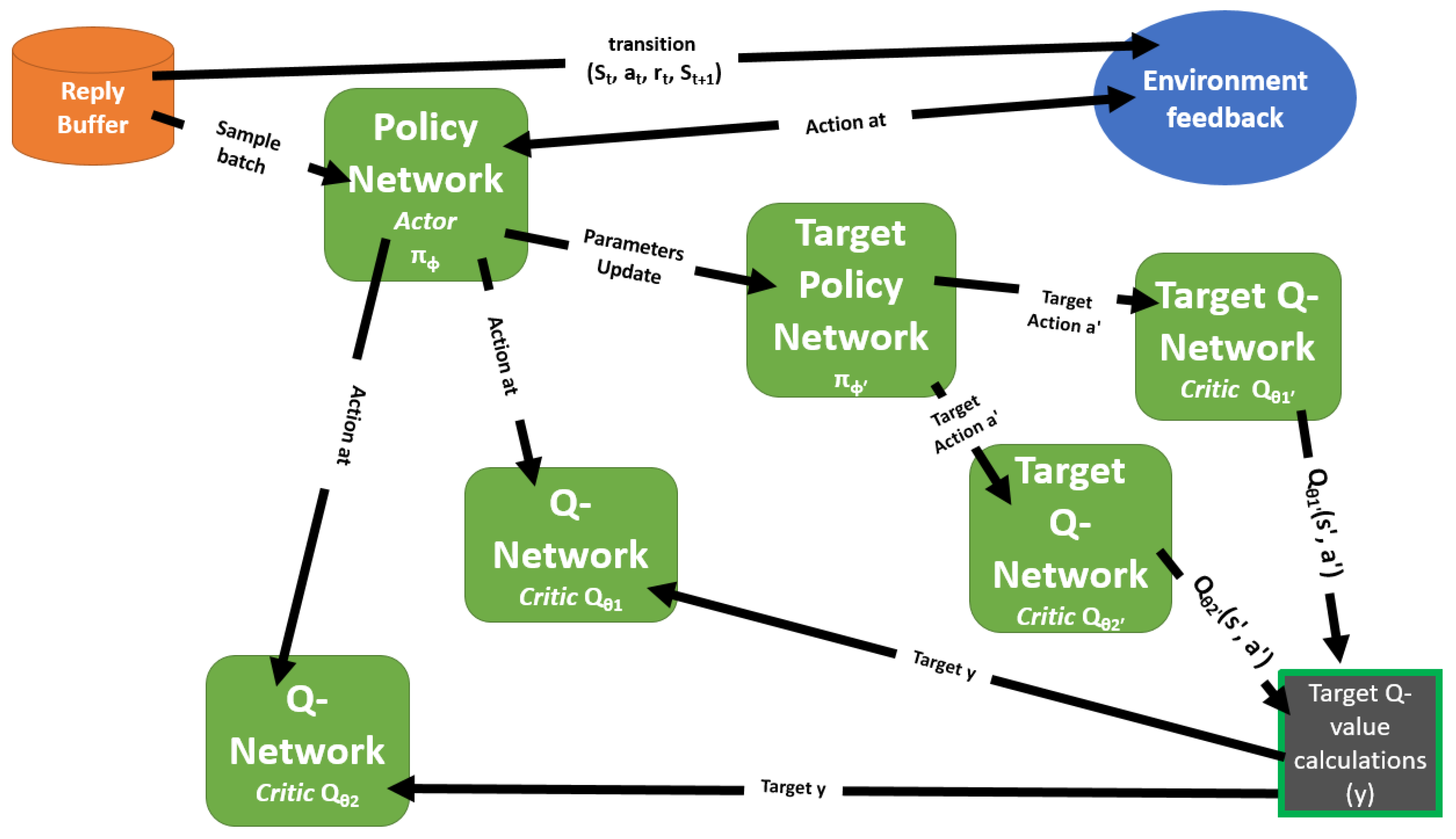
Figure 2.
Original Training Setup: Layout of four different Static Box Environments (4.5m x 4.5m) for training.
Figure 2.
Original Training Setup: Layout of four different Static Box Environments (4.5m x 4.5m) for training.
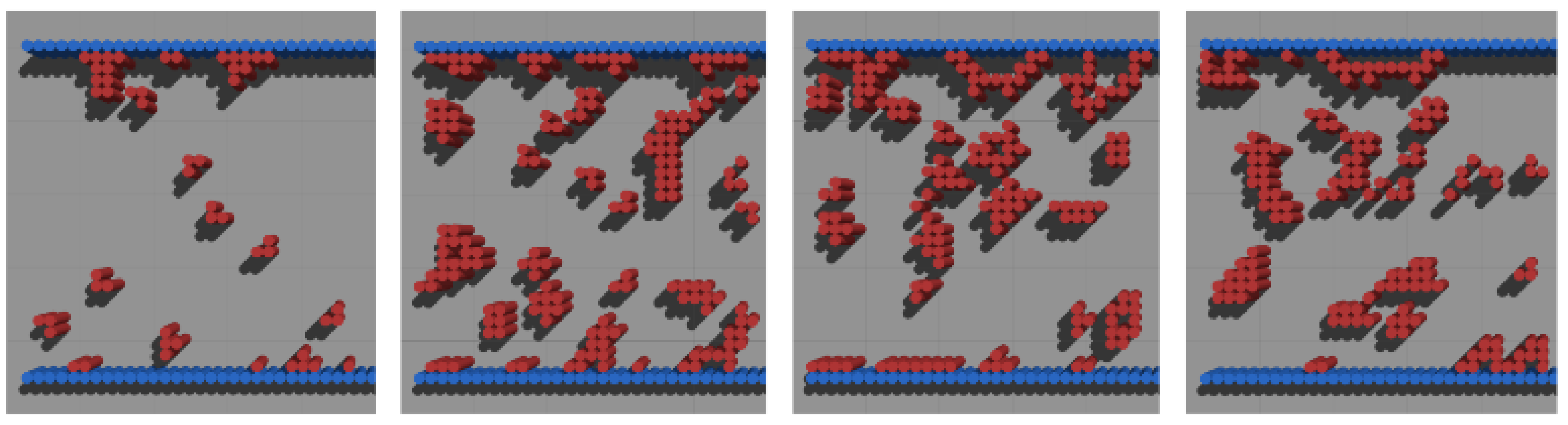
Figure 3.
Layout of the four different 16m x 16m custom static environments for training.
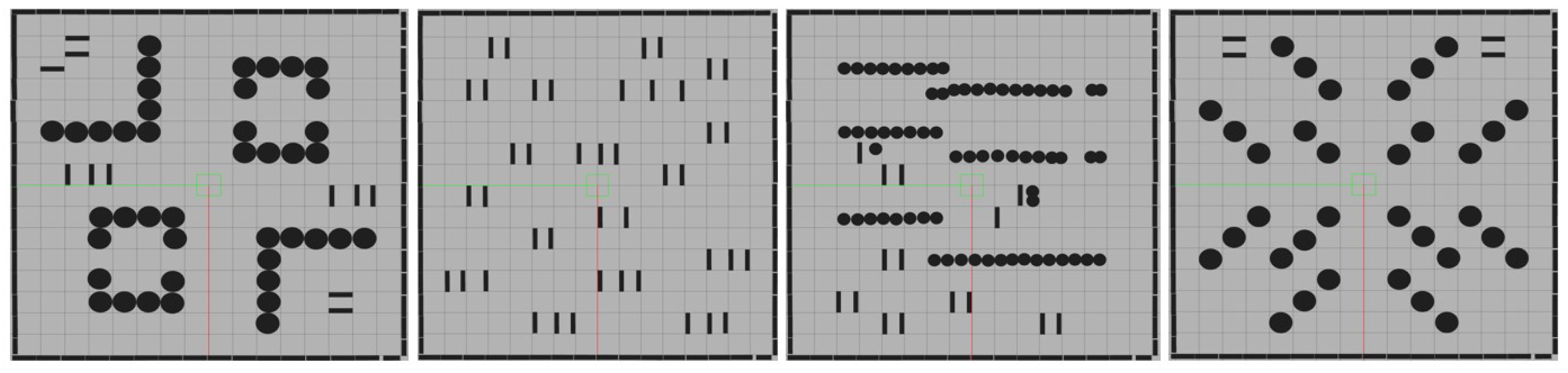
Figure 4.
Success rate comparison between the extended model (blue) and the non-extended model (orange) across training steps.
Figure 4.
Success rate comparison between the extended model (blue) and the non-extended model (orange) across training steps.
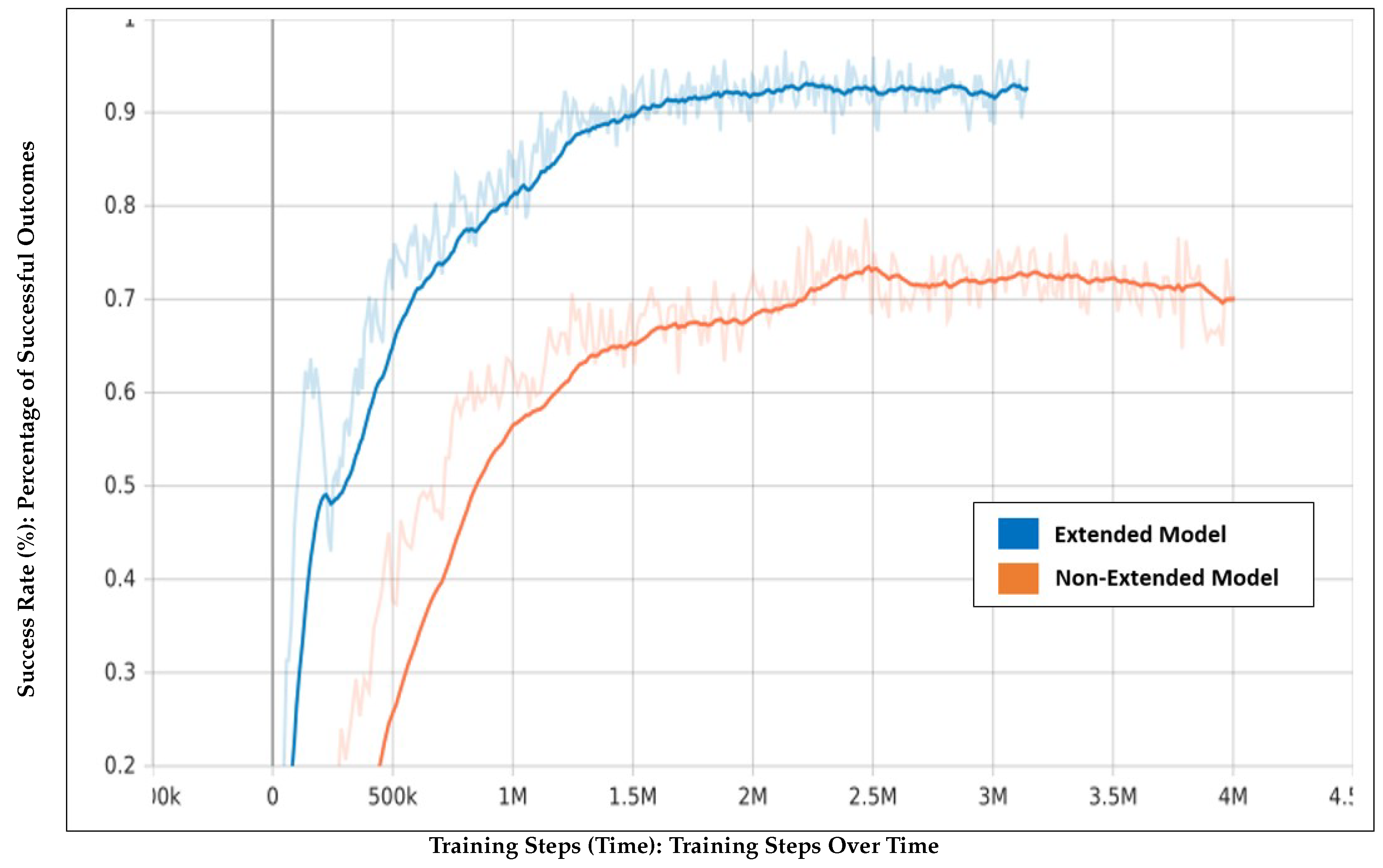
Figure 5.
Collision rate comparison between the extended model (blue) and the non-extended model (orange) across training steps.
Figure 5.
Collision rate comparison between the extended model (blue) and the non-extended model (orange) across training steps.
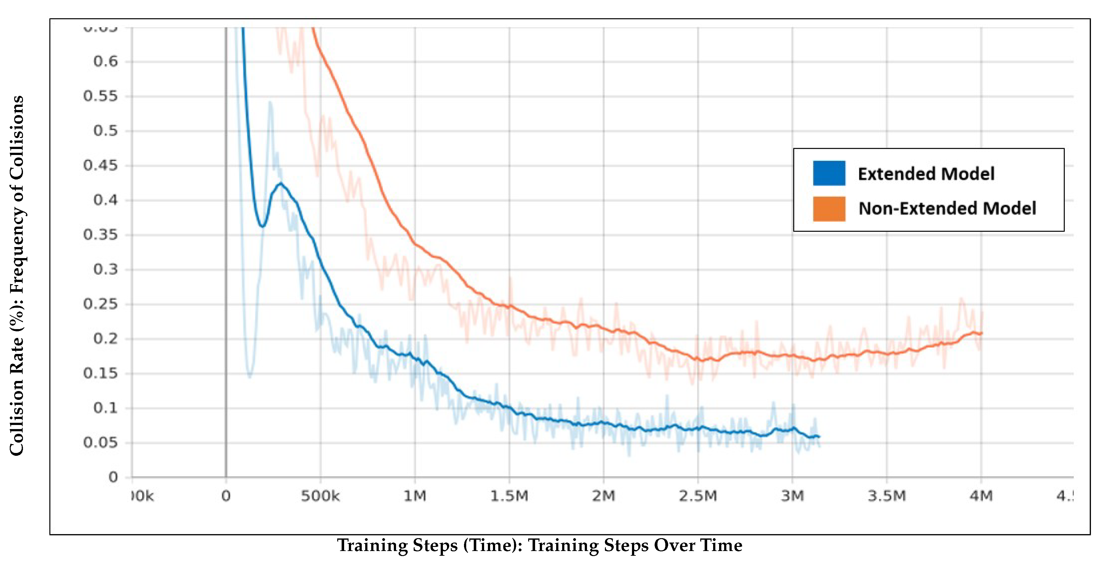
Figure 6.
Average return comparison between the extended model (blue) and the non-extended model (orange) across training steps.
Figure 6.
Average return comparison between the extended model (blue) and the non-extended model (orange) across training steps.
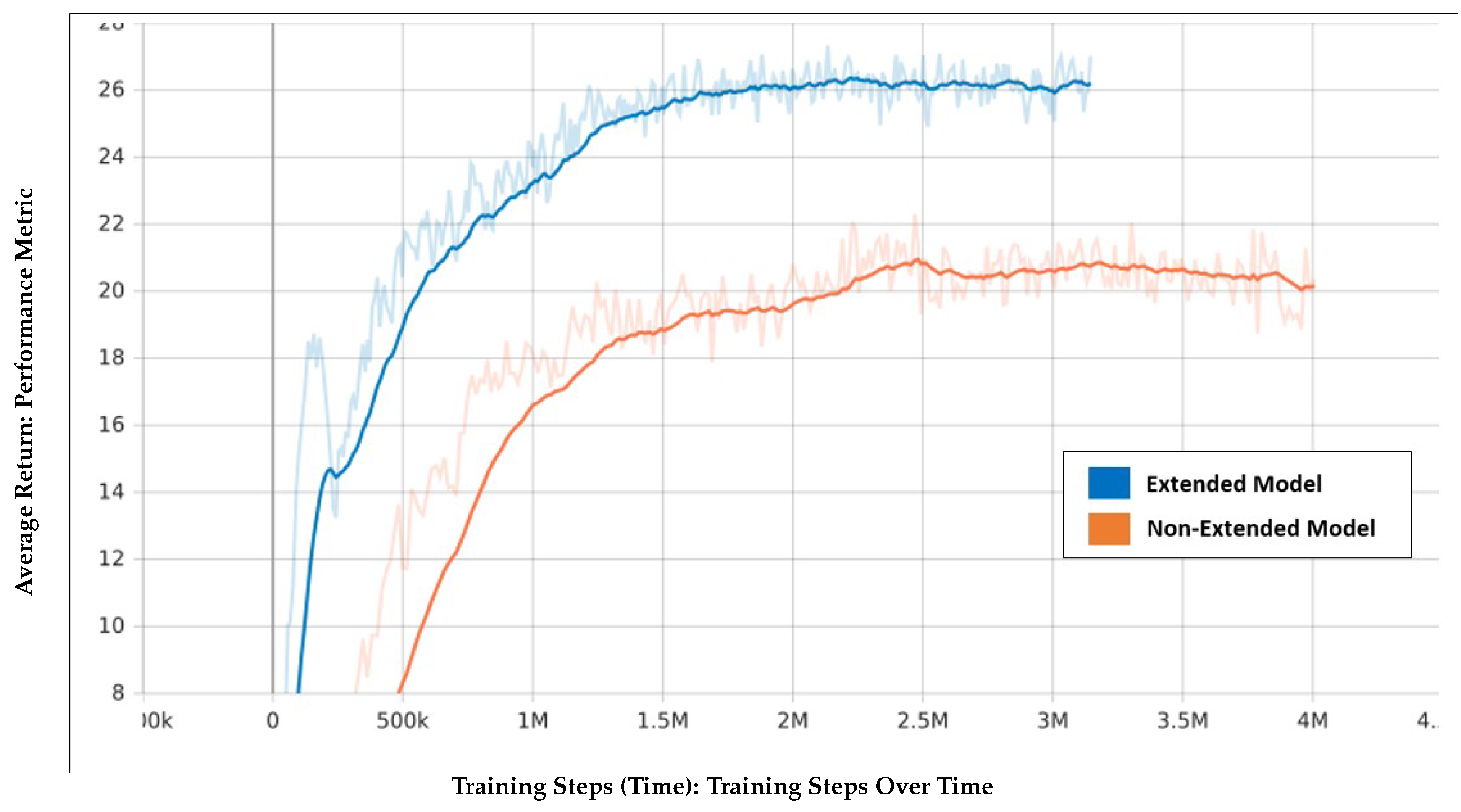
Figure 7.
Illustration of the 10 start and corresponding goal points used for evaluation in the Gazebo simulation GUI. The paths shown are intended only to indicate the connection between each start and goal point pair for both the extended and non-extended models; they do not represent the actual paths taken by the robot during evaluation, as each model followed a different route based on its learned navigation strategy.
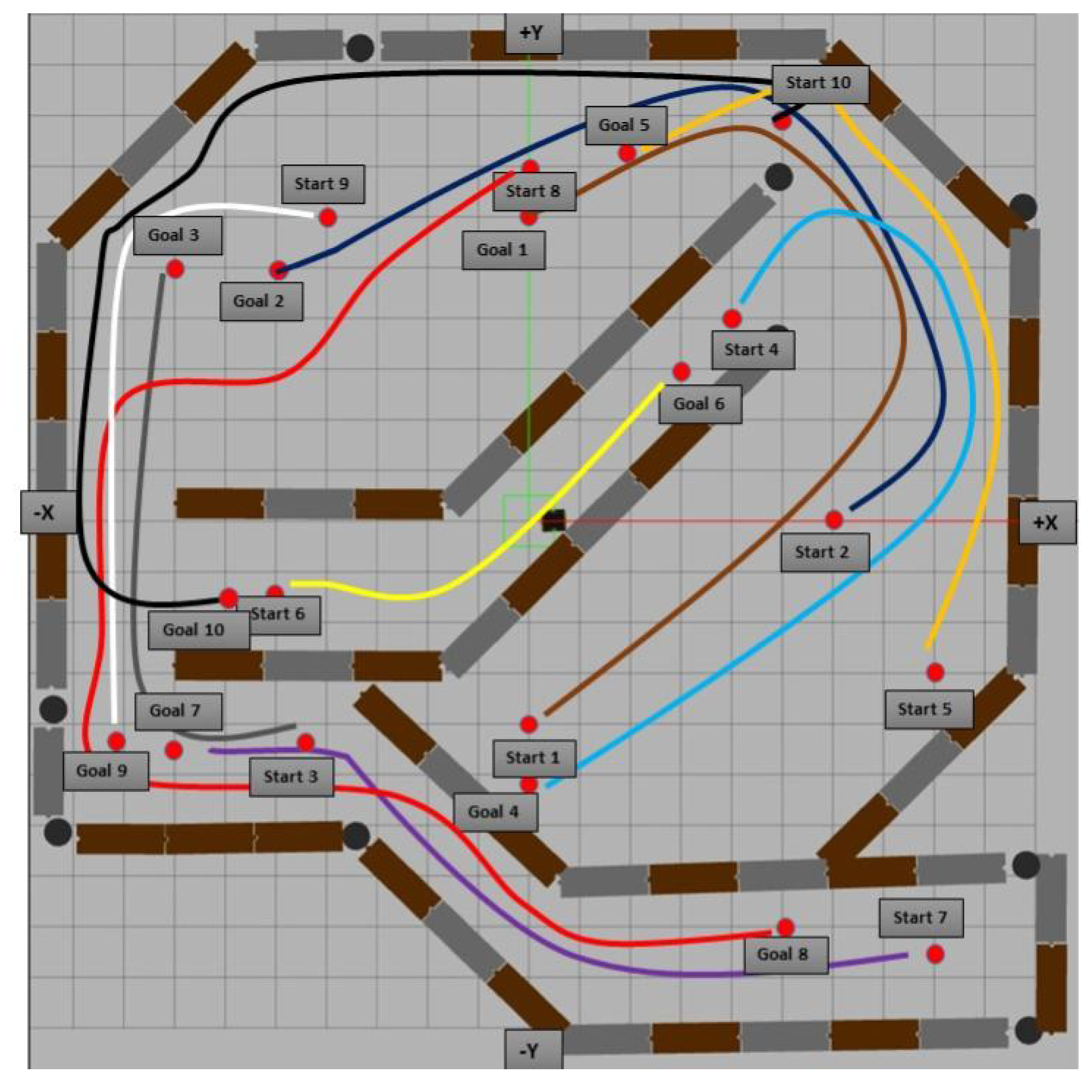
Figure 8.
Path taken by both models (Extended on the left, Not Extended on the right) for Path 1, as defined in Tables 1 and 2. The paths shown in both images are in red, illustrating the trajectory of the extended and non-extended models during evaluation. The extended model on the left demonstrates a more efficient navigation, while the non-extended model on the right shows significant deviations and exceeded the maximum allowed collisions without reaching the goal. Note: The apparent overlap of the robot’s path with the walls in the RViz visualization is a rendering artifact and does not reflect actual collisions during navigation.
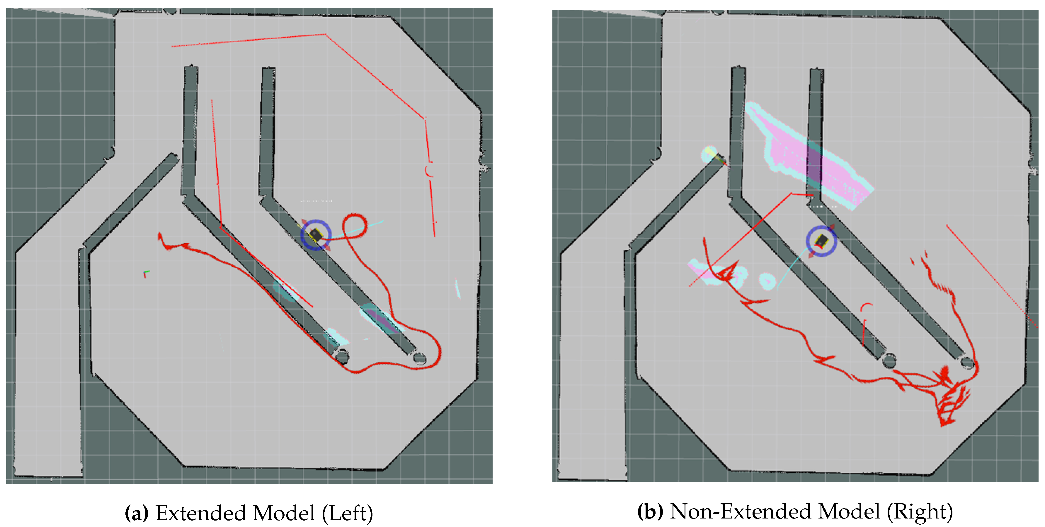
Figure 9.
Path taken by both models (Extended on the left, Not Extended on the right) for Path 2, as defined in Tables 1 and 2. The paths shown in both images are in red, illustrating the trajectory of the extended and non-extended models during evaluation. The extended model on the left demonstrates a more efficient navigation, while the non-extended model on the right shows significant deviations and timed out before reaching the goal. Note: The apparent overlap of the robot’s path with the walls in the RViz visualization seen in Figure (a) is a rendering artifact and does not represent any actual collisions during the robot’s navigation.
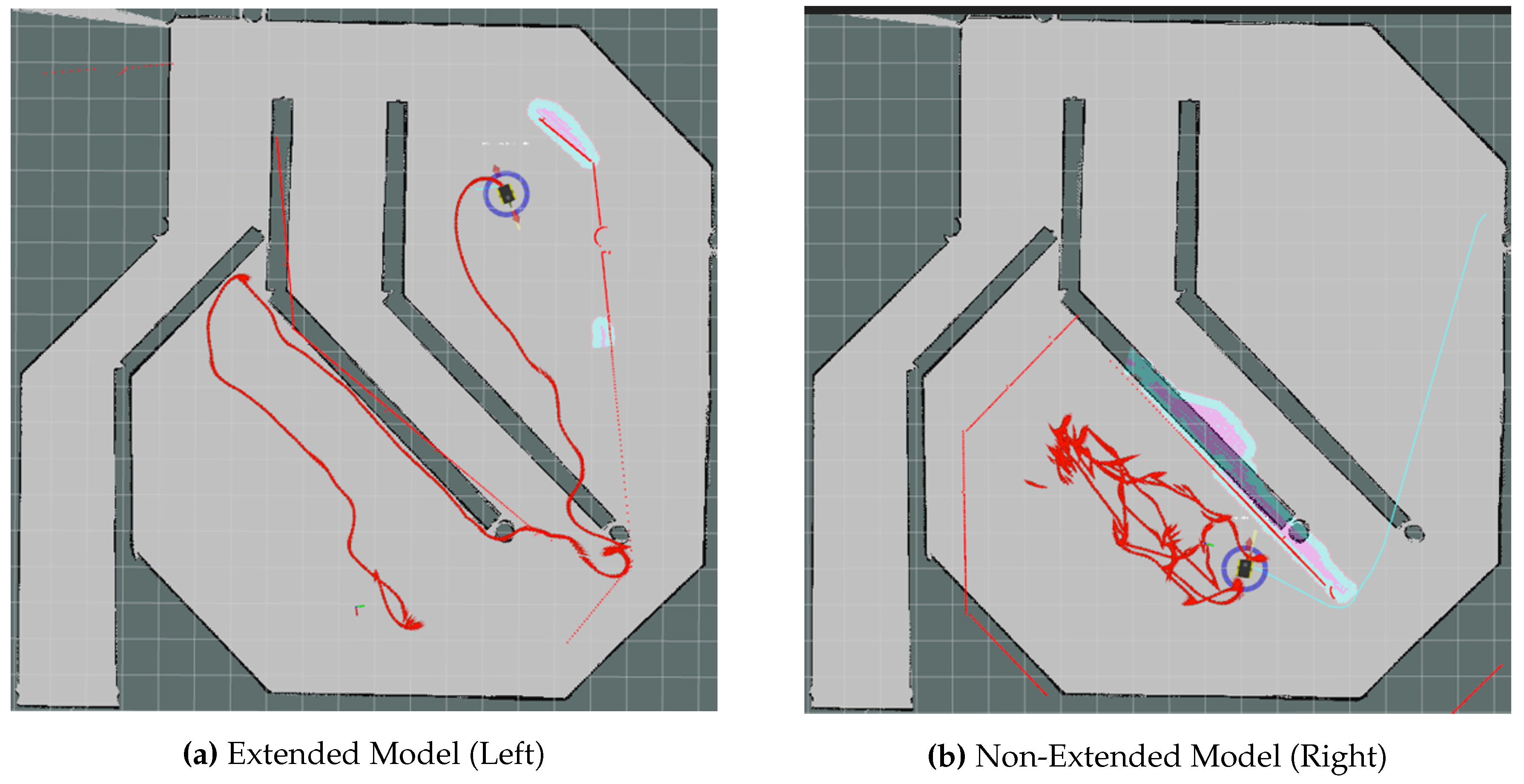

Table 1.
Test Evaluation Results for the Extended Model. Bold values indicate better performance compared to the Non-Extended Model for each metric (Distance, Collisions, Goal Reached, and Time).
Table 1.
Test Evaluation Results for the Extended Model. Bold values indicate better performance compared to the Non-Extended Model for each metric (Distance, Collisions, Goal Reached, and Time).
| Path | Distance (m) | Collisions | Goal Reached | Time (s) |
|---|---|---|---|---|
| Path 1 | 18.72 | 0 | Yes | 9.77 |
| Path 2 | 47.16 | 1 | Yes | 31.66 |
| Path 3 | 13.81 | 0 | Yes | 8.28 |
| Path 4 | 26.41 | 4 | No | 21.79 |
| Path 5 | 15.51 | 0 | Yes | 9.26 |
| Path 6 | 8.12 | 0 | Yes | 4.19 |
| Path 7 | 15.04 | 3 | Yes | 9.87 |
| Path 8 | 37.74 | 0 | No | 35.49 |
| Path 9 | 15.66 | 1 | Yes | 9.98 |
| Path 10 | 30.54 | 0 | Yes | 23.33 |
Table 2.
Test Evaluation Results for the Non-Extended Model. Bold values indicate better performance compared to the Extended Model for each metric (Distance, Collisions, Goal Reached, and Time).
Table 2.
Test Evaluation Results for the Non-Extended Model. Bold values indicate better performance compared to the Extended Model for each metric (Distance, Collisions, Goal Reached, and Time).
| Path | Distance (m) | Collisions | Goal Reached | Time (s) |
|---|---|---|---|---|
| Path 1 | 33.53 | 4 | No | 33.79 |
| Path 2 | 41.97 | 0 | No | 80.00 |
| Path 3 | 10.65 | 4 | No | 14.88 |
| Path 4 | 39.40 | 3 | No | 67.59 |
| Path 5 | 32.09 | 0 | Yes | 42.20 |
| Path 6 | 8.12 | 0 | Yes | 4.24 |
| Path 7 | 15.22 | 3 | Yes | 9.55 |
| Path 8 | 37.75 | 0 | No | 39.67 |
| Path 9 | 44.95 | 0 | No | 56.42 |
| Path 10 | 58.16 | 1 | No | 68.19 |
Table 3.
Navigation Performance Assessment Metric Scores for the Extended Model.
| Path | Metric (%) | Description |
|---|---|---|
| Path 1 | 100.00 | No collisions, within max allowed distance |
| Path 2 | 57.60 | 1 collision, exceeded optimal distance with penalty |
| Path 3 | 100.00 | No collisions, optimal path followed |
| Path 4 | 0.00 | 4 collisions, exceeded max allowed distance |
| Path 5 | 100.00 | No collisions, within optimal range |
| Path 6 | 100.00 | No collisions, optimal path |
| Path 7 | 67.00 | 3 collisions, distance exceeded slightly |
| Path 8 | 0.00 | Exceeded max allowed distance |
| Path 9 | 70.00 | 1 collision, slight penalty |
| Path 10 | 98.33 | No collisions, distance exceeded slightly |
Table 4.
Navigation Performance Assessment Metric Scores for the Non-Extended Model.
| Path | Metric (%) | Description |
|---|---|---|
| Path 1 | 0.00 | 4 collisions, exceeded max allowed distance |
| Path 2 | 0.00 | Timeout, exceeded max distance |
| Path 3 | 0.00 | 4 collisions, failed navigation |
| Path 4 | 0.00 | Exceeded max allowed distance with 3 collisions |
| Path 5 | 85.77 | No collisions, slight distance and time penalties |
| Path 6 | 100.00 | No collisions, optimal path followed |
| Path 7 | 10.00 | 3 collisions, slight penalty |
| Path 8 | 0.00 | Exceeded max allowed distance |
| Path 9 | 0.00 | Exceeded max allowed distance, timeout |
| Path 10 | 0.00 | Exceeded max allowed distance with 1 collision |
Disclaimer/Publisher’s Note: The statements, opinions and data contained in all publications are solely those of the individual author(s) and contributor(s) and not of MDPI and/or the editor(s). MDPI and/or the editor(s) disclaim responsibility for any injury to people or property resulting from any ideas, methods, instructions or products referred to in the content. |
© 2024 by the authors. Licensee MDPI, Basel, Switzerland. This article is an open access article distributed under the terms and conditions of the Creative Commons Attribution (CC BY) license (http://creativecommons.org/licenses/by/4.0/).
Copyright: This open access article is published under a Creative Commons CC BY 4.0 license, which permit the free download, distribution, and reuse, provided that the author and preprint are cited in any reuse.


