Submitted:
27 August 2025
Posted:
27 August 2025
You are already at the latest version
Abstract
When dynamic obstacles are present in the environment, traditional navigation methods often struggle to achieve safe and efficient obstacle avoidance due to their lack of real-time adaptability. To address this challenge, we propose an Ac-tion-Constrained Regularized Twin Delayed Deep Deterministic Policy Gradient (ACR-TD3) algorithm. This algorithm introduces action-constrained regularization (ACR) into the framework of the Twin Delayed Deep Deterministic Policy Gradient (TD3) to optimize navigation policies, ensuring that the robot outputs reasonable mo-tion commands and thereby reduces collision frequency, achieving higher navigation success rates. Additionally, we design a multilayer reward function, combined with the ACR, to further optimize navigation performance. Our proposed method does not rely on environmental maps and achieves end-to-end autonomous navigation based solely on LiDAR input. Experimental results demonstrate that ACR-TD3 achieves a 99% navigation success rate in simulated environments, outperforming classical algorithms such as Deep Deterministic Policy Gradient (DDPG), TD3, and Soft Actor-Critic (SAC), while also exhibiting strong generalization capabilities.
Keywords:
deep reinforcement learning
; robot navigation
; autonomous navigation
; obstacle avoidance
; LiDAR
1. Introduction
Mobile robots are currently being extensively utilized in autonomous delivery [1], cleaning [2], and rescue [3] due to rapid advancements in robotics. Mobile robots are often required for these tasks to achieve autonomous navigation and avoid both static and dynamic obstacles in the environment. The complexity and diversity of real-world application scenarios mean that, despite ongoing research on mobile robot navigation, numerous issues still require study and resolution.
Because of their dependability, traditional navigation methods [4,5,6] have been extensively employed in structured environments such as factories and warehouses during the last few decades. However, there are numerous drawbacks to this approach. The first is a lack of environmental adaptability; traditional methods often depend on precise environment modeling, which makes it challenging to deal with changes in dynamic or unfamiliar situations in real time. Second, it is hard to fulfill the real-time demands of high-speed mobile robots due to the lack of computing efficiency and real-time performance. For example, the A* algorithm has a high computational cost for path search in large-scale maps. Furthermore, the generalization power of traditional methods is limited, as they cannot automatically adapt to new environments and require manual parameter adjustments for various circumstances. Lastly, due to their limited capacity for high-dimensional sensing, traditional methods rely on human feature extraction and struggle to directly handle raw sensor data, such as vision and point clouds, which degrades performance in complicated terrain or scenarios with shifting light. Traditional methods are limited by these drawbacks in terms of their use in real-world scenarios, causing them to perform poorly in dynamic situations.
Deep Reinforcement Learning (DRL) offers a new technical avenue for mobile robot navigation by combining the superior decision-making capabilities of reinforcement learning with the potent perceptual capabilities of deep neural networks. DRL exhibits notable benefits over traditional methods in terms of generalization ability, computational economy, and environmental flexibility [7,8,9]. DRL can better adapt to dynamic situations by learning environmental properties directly from raw sensor data, eliminating the need for environment modeling and laborious feature extraction. In addition, DRL is capable of long-term planning, which may balance path optimization with real-time decision-making by implicitly learning long-term rewards through value functions or actor networks. Finally, the trained model may be transferred to similar but untrained environments and perform well, demonstrating DRL’s great generalization capabilities.
Although DRL-based techniques have shown promise in autonomous robot navigation, they still face challenges such as trouble navigating in dynamic environments and a propensity for local optimization. To address these challenges, we proposed a DRL-based mobile robot navigation algorithm, ACR-TD3, which optimizes the training process of the actor network and achieves a higher navigation success rate by introducing an ACR in the TD3 algorithm; at the same time, we design a multilayer reward function, which, combined with ACR, improves navigation performance in dynamic environments.
2. Related Work
In 2005, Garulli et al. [10] proposed a line-feature-based simultaneous localization and mapping (SLAM) method that uses Extended Kalman Filtering (EKF) to facilitate localization and map construction in structured environments while minimizing computational complexity. Harik et al. [11] integrated Hector SLAM with Artificial Potential Field (APF) to provide real-time navigation and obstacle avoidance in greenhouse conditions. Kim et al. [12] proposed an end-to-end deep learning model to anticipate control instructions directly from sensor data, which decreases the error accumulation of typical navigation modules. Wang et al. [13] proposed an end-to-end deep neural network controller utilizing LiDAR, which establishes a direct sensor-to-action mapping for robotic navigation. Nonetheless, these methods depend on precise environmental modeling, exhibit significant computing complexity, and often underperform when confronted with dynamic impediments and unstructured environments, hence complicating the fulfillment of real-time and robustness requirements.
DRL was introduced by Minh et al. [14] in 2013 during the gameplay of an Atari game. The intelligence model was able to effectively acquire control methods from the game environment and surpassed human performance in certain games. In 2016, Tai, L. et al. [15] first implemented DRL for robot navigation, demonstrating the viability of mapless navigation in both simulated and real-world environments. Subsequently, [16] employed DRL for goal-driven visual navigation utilizing RGB and target pictures as inputs and acquired navigation strategies via a Siamese network, establishing a basis for future vision-based DRL navigation studies. The authors of [17] proposed an end-to-end methodology of DRL to navigate a mobile robot in an unfamiliar area with an RGB camera for environmental sensing. Nonetheless, RGB-based methods exhibit inadequate generalization capabilities, and a substantial disparity in navigation performance exists in real-world and virtual environments.
Therefore, multiple scholars have endeavored to enhance generalizability. One method involves using a depth camera to obtain environmental data. A Convolutional Deep Deterministic Policy Gradient (CDDPG) network [18] was proposed to process extensive depth image data, successfully circumventing both static and dynamic barriers. The authors of [19] proposed a binocular vision-based steering control system for autonomous driving, enabling end-to-end autonomous steering decision-making using an enhanced Deep Deterministic Policy Gradient (DDPG) network. Nevertheless, depth image-based techniques sometimes need intricate convolutional processes to analyze visual data, resulting in significant processing demands, which creates a notable performance limitation in real-world navigation applications. Conversely, LiDAR has emerged as an efficient alternative to improve the generalization of DRL navigation owing to its exceptional precision, rapid responsiveness, and robust anti-jamming capabilities. The authors of [20] proposed a DRL navigation technique utilizing LiDAR and RGB cameras, achieving autonomous navigation from basic memory to intricate reasoning in indoor environments via a memory-reasoning framework. The authors of [21] used fused data from LiDAR and RGB cameras as inputs for the robot, subsequently incorporating random Gaussian noise into the incoming laser data to improve resilience and navigation. Nonetheless, multimodal sensor fusion not only increases computational demands but may also induce calibration drift in dynamic environments. The authors of [22] proposed an optimization method for navigation policy utilizing LiDAR and DRL frameworks that rapidly adapts to human preferences, enabling dynamic adjustments of navigation behaviors in a robot. In addition, the authors of [23] proposed a crowd-aware navigation system utilizing LiDAR and memory-enhanced DRL, effectively achieving navigation in a densely populated area, while the authors of [24] proposed the iTD3-CLN framework, which integrates LiDAR and TD3 to provide mapless autonomous navigation in dynamic situations with little reliance on accurate sensors. The authors of [25] proposed a navigation method that integrates imitation learning and DRL for motion planning in congested environments. By independently processing information on static and dynamic objects, the network may acquire motion patterns appropriate for real-world environments. The SAC-DRL system proposed in [26] incorporates LiDAR perception and exhibits enhanced stability and flexibility in navigating challenging terrains. This paper builds upon LiDAR technology and presents ACR-TD3, which incorporates ACR into the TD3 algorithm to optimize the navigation policy, enabling the robot to consistently generate accurate action commands and successfully navigate dynamic environments.
3. Materials and Methods
To achieve autonomous navigation of mobile robots in mapless dynamic environments, we proposed a DRL-based navigation algorithm, ACR-TD3, which optimizes the navigation policy by incorporating ACR into the actor loss of the TD3 network. This modification enables the actor network to generate more rational motion commands, thereby increasing the success rate of navigation in dynamic environments. Concurrently, we develop a multilayer reward function integrated with ACR to improve navigation efficacy.
3.1. ACR-TD3
Within the DRL framework, the essence of the mobile robot navigation challenge is to identify the optimal policy using a policy optimization technique that maximizes the anticipated cumulative return achieved by the agent in the Markov Decision Process (MDP). The merits and demerits of this navigation technique directly influence the efficacy of mobile robot navigation. In TD3, the objective of the policy is to optimize the Q-value, specifically to identify the action that maximizes the Q-value output of the critic network, while the optimizer is often employed to minimize the loss, necessitating the usage of negative values to convert the issue into a minimization framework. Consequently, the actor loss function is articulated as follows:
where is the input state, is the deterministic action output by the actor network, and is the Q-value of the first value network output of TD3.
During the primary phases of training, the parameters of the actor network are iteratively refined via gradient ascent to optimize policy efficacy. Model training is deemed complete when the policy performance metric stabilizes within a defined range and the Bellman error decreases below a certain threshold. At this juncture, the actor network attains a near-optimal state and is capable of producing a consistent sequence of navigation decisions. Nevertheless, the action orders produced by the existing policy typically exhibit suboptimal performance, often resulting in accidents due to inadequate time to evade moving impediments, thereby compromising navigation efficacy in dynamic environments. To resolve this issue, we include ACR into the TD3 algorithm, incorporating it into the actor loss function to optimize the navigation policy. This allows the actor network to provide more rational movement orders, thereby improving navigation efficacy in dynamic environments. The complete network structure of ACR-TD3 is shown in Figure 1.
The new actor loss following the implementation of ACR is defined as follows:
ACR primarily optimizes the policy by limiting the angular and linear velocities inside the action space, achieving smooth and rational behaviors from the actor network following policy changes. ACR can be articulated as follows:
The ACR consists of three parts: smoothing loss, obstacle distance loss, and action boundary loss, with corresponding coefficients of , , and , respectively. Reducing velocity mutation, smoothing the navigation route, and preventing collisions or lengthier navigation trajectories caused by frequent velocity changes are the goals of adding smoothing loss. Each step’s loss is determined by calculating the square of the velocity difference between the current and previous moments, or the square of the velocity change between two adjacent steps. The smoothing loss at each episode is then calculated by averaging the loss at each step. The expression for the smoothing loss is
where represents the change in linear velocity between two adjacent steps, while signifies the change in angular velocity between two adjacent steps. Incorporating and into the smoothing loss term can effectively mitigate abrupt changes in the robot’s velocity. The obstacle distance loss is implemented to maintain a specified distance between the mobile robot and obstacles, providing the robot with adequate reaction time to address approaching dynamic obstacles, thereby enhancing the success rate and navigation safety. The obstacle distance loss can be articulated as follows:
whereis the distance to the nearest obstacle acquired from LiDAR at the moment, andis the distance threshold. In order to impose restrictions on the robot’s movement close to the obstacle and simultaneously encourage the robot to maintain a relatively safe distance from the obstacle, we set as a segmented function. When the distance between the robot and the nearest obstacle is smaller than the preset distance threshold, it will achieve a larger loss, and the loss will increase linearly as the distance becomes closer; when the distance between the robot and the nearest obstacle is larger than the preset distance threshold, it will achieve a smaller loss, and the loss will decrease exponentially as the distance increases. Therefore, the robot will choose the action with a distance greater than from the obstacle to minimize the loss, thus guaranteeing the safety of navigation. The action boundary loss is introduced to place a limit on the size of the robot’s linear and angular velocities. Excessive linear velocity will cause the robot to break the distance threshold in a short time, and the robot will collide head-on with the dynamic obstacle when it comes close because it is too late to avoid it; excessive angular velocity will cause the robot to over-adjust its direction, which will lead to frequent direction corrections afterward and ultimately affect its navigation. The action boundary loss can be expressed as follows:
whereanddenote the linear and angular velocities, respectively, at time. Linear velocities of 0.5 meters per second are within the allowable range of the robot’s design, and therefore, losses are imposed only when the linear velocity is greater than 0.5 meters per second.
3.2. Reward Functions
The design of reward functions is particularly crucial due to the numerous uncertainties present in dynamic environments. We examined several parameters influencing navigation in dynamic environments and meticulously developed a multilayer reward function, delineated as follows:
The multilayer rewards encompass termination awards, heading angle rewards, target distance rewards, obstacle distance rewards, linear velocity rewards, angular velocity rewards, and decay rewards. The termination awards, often referred to as sparse rewards, are assigned to the robot according to the navigation outcomes (success, collision, or timeout) of each episode, indicated as:
A positive reward is awarded to the robot if it successfully reaches the target location, while a negative reward is awarded if the robot collides with an obstacle. If the robot fails to complete the task within the designated time frame, it is deemed to have exceeded the time limit and is awarded a 0 reward.
Nonetheless, confining sparse rewards solely to the robot is insufficient. The absence of reward guidance during navigation impacts the robot’s ability to explore the target location randomly in the early stages of training, resulting in a predominance of 0 rewards, which considerably diminishes learning efficiency. Furthermore, this may induce an unstable training process, leading the policy update to converge to a local optimum. To avoid these problems, we add the necessary dense rewards to the sparse rewards, including heading angle rewards, target distance rewards, obstacle distance rewards, linear velocity rewards, angular velocity rewards, and decay rewards. These dense rewards are all designed to make the robot explore more purposefully and improve its learning efficiency.
The heading angle reward ©s used to encourage the robot to move ©n the direction of the goal to minimize roaming or detours. The representation is as follows:
where denotes the angle between the robot’s forward direction and the target direction, i.e., the heading angle, and the larger the angle , the larger the negative reward the robot receives. The target distance reward measures the reward obtained by calculating the Euclidean distance between the robot and the target, which is used to encourage the robot to approach the target step by step, and can be expressed as follows:
where denotes the distance between the robot and the target location. When a moving obstacle approaches head-on towards the robot, the robot often hits the moving obstacle because it is too late to avoid it. Therefore, an obstacle distance reward is set for penalizing the robot for getting too close to an obstacle and is denoted as follows:
When the distance to the nearest obstacle is less than the distance threshold, the robot receives a larger negative reward, and the closer the robot is to the obstacle, the larger the negative reward is; when is larger than, the robot receives a negative reward that decreases exponentially as increases. The linear and angular velocity rewards are used to penalize sudden velocity changes and keep the robot running smoothly. The linear velocity reward is denoted as follows:
is the desired linear velocity, and the larger the deviation of the actual linear velocity from the desired linear velocity, the larger the negative reward received. In particular, if the robot’s linear velocity is less than 0.05 meters per second, the robot is considered to rotate in place or stay in place, which is not allowed, and therefore, a fixed negative reward is given. The angular velocity reward is denoted as follows:
This is used to penalize the robot for frequently changing the direction of movement. Finally, for better navigation, we also add a decaying reward, which gives a constant negative reward for each step of the robot to urge the robot to reach the goal as soon as possible.
4. Training
In addition to being costly and risky for robots, training in real-world environments is also hazardous for people and the environment. In order to address this problem, we trained the proposed model in a 6x6 m2 simulated environment in Gazebo [27], as seen in Figure 2. The machine has an Intel Core i9-10900K CPU, an NVIDIA GeForce RTX 3090 GPU, and 64 GB of RAM. PyTorch is the training framework utilized [28]. We interact with the simulated world using a TurtleBot 3 robot that is outfitted with odometry and LiDAR. The robot’s control and communication architecture is the Robot Operating System 2 (ROS 2) [29], which is mainly used to publish target position information, subscribe to messages from the LiDAR and odometer, and publish linear and angular velocity information to regulate the robot’s movements.
At the start of each episode, the target position is published via ROS 2 and marked as a red point in the training environment. Simultaneously, the dynamic obstacle begins to move along the specified path, and the robot starts navigation training from the center position. During training, the robot’s maximum linear velocity is set to 0.5 meters per second, and the maximum angular velocity is set to 2 radians per second. Key information for each step is stored in a replay buffer with a capacity of 2e6 in the form of an array, where and represent the current state and action, represents the current reward, represents the next state, and indicates whether the episode has ended. When the buffer reaches capacity, new data supersedes the existing data. Three scenarios cause the episode to end: success, collision, and timeout. If the robot is within 0.2 meters of the target, it is considered to have successfully reached the target, the episode ends, and a success rewardis granted; if the robot is within 0.13 meters of an obstacle, it is considered to have collided, the episode ends, and a collision rewardis granted; and if the episode has not ended after 50 seconds, it is considered a timeout, the episode is forced to end, and no rewards are granted. The network parameters used for model training are shown in Table 1. We performed training until the model converged, which required approximately 6,000 episodes, and this took about 27 hours.
5. Experiments
We created three test scenarios of differing complexity within the Gazebo simulation platform to assess the proposed approach, as seen in Figure 3. The test environments retain the same physical dimensions (8×6 m2) and a consistent number of static obstacles; however, they vary in the arrangement of static obstacles and the quantity of dynamic obstacles. Figure 3(a) depicts four dynamic obstacles and six static obstacles, categorized as a simple environment (Env1); Figure 3(b) illustrates six dynamic obstacles and six static obstacles, classified as a medium-difficulty environment (Env2); and Figure 3(c) presents eight dynamic obstacles and six static obstacles, designated as a difficult environment (Env3).
We tested the trained model in the environment shown in Figure 3. Each environment performed 100 independent navigation tasks and was repeated three times to eliminate random errors. The test results are recorded in Figure 4.
Figure 4 shows that our proposed ACR-TD3 surpasses the other three algorithms in the number of successful navigation occurrences across all three environments, indicating superior performance in dynamic environments. To provide a clearer comparison of navigation performance, we recorded the model’s navigation success rate and trajectory length after the application of a moving average in Table 2 and Table 3. Table 2 shows that in the comparatively straightforward Env1 and the moderately challenging Env2 environments, our model attained navigation success rates of 99% and 98%, respectively, surpassing other models. Despite the arduous Env3 environment, our suggested model achieved a navigation success rate of 96.7%, surpassing the best-performing model by 6.33% under identical conditions. Furthermore, as seen in Table 3, our model exhibits a reduced trajectory length in comparison to other models, reinforcing the superiority of ACR-TD3.
The previous analysis shows that ACR-TD3 performs well in terms of navigation success rate, trajectory length, and environmental adaptability, validating the effectiveness of ACR-TD3 for navigation in dynamic environments and providing a new solution for mobile robot navigation in dynamic environments.
6. Conclusions
This paper proposes a DRL algorithm that incorporates ACR. By utilizing LiDAR to obtain environmental information, it achieves end-to-end autonomous navigation in dynamic environments. The algorithm innovatively integrates an action space constraint mechanism with a multilayer reward function design, effectively improving navigation success rates and efficiency without the need for pre-constructed maps. For experiments, we created a dynamic environment using the Gazebo simulation platform to assess the algorithm’s efficacy. The experimental findings exhibited the superiority of the proposed model regarding the success rate and generalization capability. Owing to constraints in the experimental context, the approach was verified solely through simulation. Future studies should concentrate on verifying the algorithm on actual robotic platforms, such as TurtleBot 3, to augment its applicability.
Author Contributions
Conceptualization, L.D. and M.C.; methodology, L.D.; software, L.D.; validation, L.D.; formal analysis, M.C.; resources, M.C.; data curation, L.D.; writing—original draft preparation, L.D.; writing—review and editing, M.C.; project administration, M.C.; funding acquisition, M.C. All authors have read and agreed to the published version of the manuscript.
Funding
This research was funded by Hubei Provincial Central Guidance Local Science and Technology Development Project (No. 2024BSB002).
Data Availability Statement
The original contributions presented in the study are included in the article; further inquiries can be directed to the corresponding author.
Conflicts of Interest
The authors declare no conflicts of interest.
References
- Chen, Z.; Gan, Y.; Dong, S. Optimization of Mobile Robot Delivery System Based on Deep Learning. J. Comput. Sci. Res. 2024, 6, 51–65.
- Cimurs, R.; Merchán-Cruz, E.A. Leveraging Expert Demonstration Features for Deep Reinforcement Learning in Floor Cleaning Robot Navigation. Sensors 2022, 22, 7750.
- Abdeh, M.; Abut, F.; Akay, F. Autonomous Navigation in Search and Rescue Simulated Environment Using Deep Reinforcement Learning. Balkan J. Electr. Comput. Eng. 2021, 9, 92–98.
- Zhai, H.-Q.; Wang, L.-H. The Robust Residual-Based Adaptive Estimation Kalman Filter Method for Strap-Down Inertial and Geomagnetic Tightly Integrated Navigation System. Rev. Sci. Instrum. 2020, 91, 10.
- Bai, Y.; Zhang, H.; Wu, J.; Yang, W. UAV Path Planning Based on Improved A* and DWA Algorithms. Int. J. Aerosp. Eng. 2021, 2021, 4511252.
- Li, B.; Chen, B. An Adaptive Rapidly-Exploring Random Tree. IEEE/CAA J. Autom. Sin. 2022, 9, 283–294.
- Plasencia-Salgueiro, A.J. Deep Reinforcement Learning for Autonomous Mobile Robot Navigation. In Artificial Intelligence for Robotics and Autonomous Systems Applications; Springer: Cham, Switzerland, 2023; pp. 195–237.
- Ranaweera, M.; Mahmoud, Q.H. Virtual to Real-World Transfer Learning: A Systematic Review. Electronics 2021, 10, 1491.
- James, S.; Wohlhart, P.; Kalakrishnan, M.; Kalashnikov, D.; Irpan, A.; Ibarz, J.; et al. Sim-to-Real via Sim-to-Sim: Data-Efficient Robotic Grasping via Randomized-to-Canonical Adaptation Networks. In Proc. IEEE/CVF Conf. Comput. Vis. Pattern Recognit. 2019, 12619–12629.
- Garulli, A.; Giannitrapani, A.; Prattichizzo, D.; Vicino, A. Mobile Robot SLAM for Line-Based Environment Representation. In Proceedings of the 44th IEEE Conference on Decision and Control (CDC), Seville, Spain, 2005; pp. 2041–2046.
- Harik, E.H.; Korsaeth, A. Combining Hector SLAM and Artificial Potential Field for Autonomous Navigation Inside a Greenhouse. Robotics 2018, 7, 22.
- Kim, Y.-H.; Jang, J.-I.; Yun, S. End-to-End Deep Learning for Autonomous Navigation of Mobile Robot. In Proceedings of the 2018 IEEE International Conference on Consumer Electronics (ICCE), Las Vegas, NV, USA, 12–14 January 2018; pp. 1–6.
- Wang, J.K.; Zhang, X.; Zhao, Y.; Li, H.; Guo, K. A LiDAR-Based End-to-End Controller for Robot Navigation Using Deep Neural Network. In Proceedings of the 2017 IEEE International Conference on Unmanned Systems (ICUS), Beijing, China, 27–29 October 2017; pp. 302–307.
- Mnih, V.; Kavukcuoglu, K.; Silver, D.; Rusu, A.A.; Veness, J.; Bellemare, M.G.; Graves, A.; Riedmiller, M.; Fidjeland, A.K.; Ostrovski, G.; et al. Human-Level Control Through Deep Reinforcement Learning. Nature 2015, 518, 529–533.
- Tai, L.; Li, S.; Liu, M. A Deep-Network Solution Towards Model-Less Obstacle Avoidance. In Proceedings of the 2016 IEEE/RSJ International Conference on Intelligent Robots and Systems (IROS), Daejeon, Republic of Korea, 9–14 October 2016; pp. 2759–2764.
- Zhu, Y.; Mottaghi, R.; Kolve, E.; Lim, J.J.; Gupta, A.; Fei-Fei, L.; Farhadi, A. Target-Driven Visual Navigation in Indoor Scenes Using Deep Reinforcement Learning. In Proceedings of the 2017 IEEE International Conference on Robotics and Automation (ICRA), Singapore, 29 May–3 June 2017; pp. 3357–3364.
- Ruan, X.; Zhang, Y.; Zhang, Z.; Zhou, X. Mobile Robot Navigation Based on Deep Reinforcement Learning. In Proceedings of the 2019 Chinese Control and Decision Conference (CCDC), Nanchang, China, 3–5 June 2019; pp. 5803–5808.
- Cimurs, R.; Suh, I.H.; Lee, S.H. Goal-Driven Autonomous Exploration Through Deep Reinforcement Learning. IEEE Robot. Autom. Lett. 2021, 7, 730–737.
- Wu, K.; Wang, X.; Zhang, S.; Huang, K. BND*-DDQN: Learn to Steer Autonomously Through Deep Reinforcement Learning. IEEE Trans. Cogn. Dev. Syst. 2019, 13, 249–261.
- Ma, L.; Zhao, T.; Wang, Y.; Wang, X.; Zhao, H.; Wang, Y. Learning to Navigate in Indoor Environments: From Memorizing to Reasoning. arXiv 2019, arXiv:1904.06933.
- Surmann, H.; Pörtner, A.; Pfingsthorn, M.; Wünsche, H. Deep Reinforcement Learning for Real Autonomous Mobile Robot Navigation in Indoor Environments. arXiv 2020, arXiv:2005.13857.
- Choi, J.; Dance, C.; Kim, J.E.; Park, K.S.; Han, J.; Seo, J.; et al. Fast Adaptation of Deep Reinforcement Learning-Based Navigation Skills to Human Preference. In Proc. IEEE Int. Conf. Robotics Autom. (ICRA), 2020; pp. 3363–3370.
- Samsani, S.S.; Mutahira, H.; Muhammad, M.S. Memory-Based Crowd-Aware Robot Navigation Using Deep Reinforcement Learning. Complex Intell. Syst. 2023, 9, 2147–2158.
- Jiang, H.; Ding, Z.; Cao, Z.; Liu, H. iTD3-CLN: Learn to Navigate in Dynamic Scene Through Deep Reinforcement Learning. Neurocomputing 2022, 503, 118–128.
- Liu, L.; Lin, H.; Zhang, M.; Wang, H.; Li, L.; Wang, Z. Robot Navigation in Crowded Environments Using Deep Reinforcement Learning. In Proceedings of the 2020 IEEE/RSJ International Conference on Intelligent Robots and Systems (IROS), Las Vegas, NV, USA, 25–29 October 2020; pp. 11349–11355.
- Liu, Y.; Zhang, X.; Yu, D.; Xu, W.; Lu, Y.; Song, Y. A Soft Actor-Critic Deep Reinforcement-Learning-Based Robot Navigation Method Using LiDAR. Remote Sens. 2024, 16, 2072.
- Koenig, N.; Howard, A. Design and Use Paradigms for Gazebo, an Open-Source Multi-Robot Simulator. In Proceedings of the 2004 IEEE/RSJ International Conference on Intelligent Robots and Systems (IROS), Sendai, Japan, 28 September–2 October 2004; Volume 3, pp. 2149–2154.
- Paszke, A.; Gross, S.; Massa, F.; Lerer, A.; Bradbury, J.; Chanan, G.; Killeen, T.; Lin, Z.; Gimelshein, N.; Antiga, L.; et al. PyTorch: An Imperative Style, High-Performance Deep Learning Library. In Adv. Neural Inf. Process. Syst. 2019, 32, 8024–8035.
- Puck, L.; Walther, D.; Lüdtke, D.; Schlegel, C. Distributed and Synchronized Setup Towards Real-Time Robotic Control Using ROS2 on Linux. In Proceedings of the 2020 IEEE 16th International Conference on Automation Science and Engineering (CASE), Hong Kong, China, 20–21 August 2020; pp. 351–358.
Figure 1.
ACR-TD3 algorithm network structure with actor and critic parts. The new actor loss is obtained by combining ACR with the original actor loss.
Figure 1.
ACR-TD3 algorithm network structure with actor and critic parts. The new actor loss is obtained by combining ACR with the original actor loss.
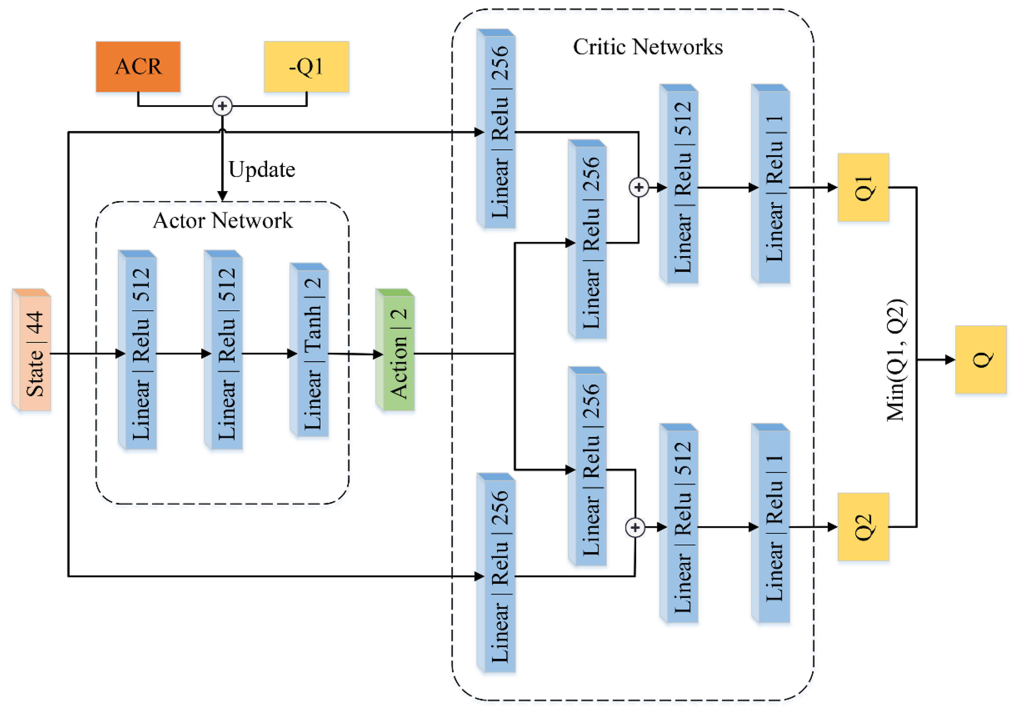
Figure 2.
In the training environment, the brick-red rectangles represent walls that double as static barriers, the white cylindrical objects represent dynamic obstacles, the red points represent target locations, and the blue regions represent the LiDAR’s sample range.
Figure 2.
In the training environment, the brick-red rectangles represent walls that double as static barriers, the white cylindrical objects represent dynamic obstacles, the red points represent target locations, and the blue regions represent the LiDAR’s sample range.
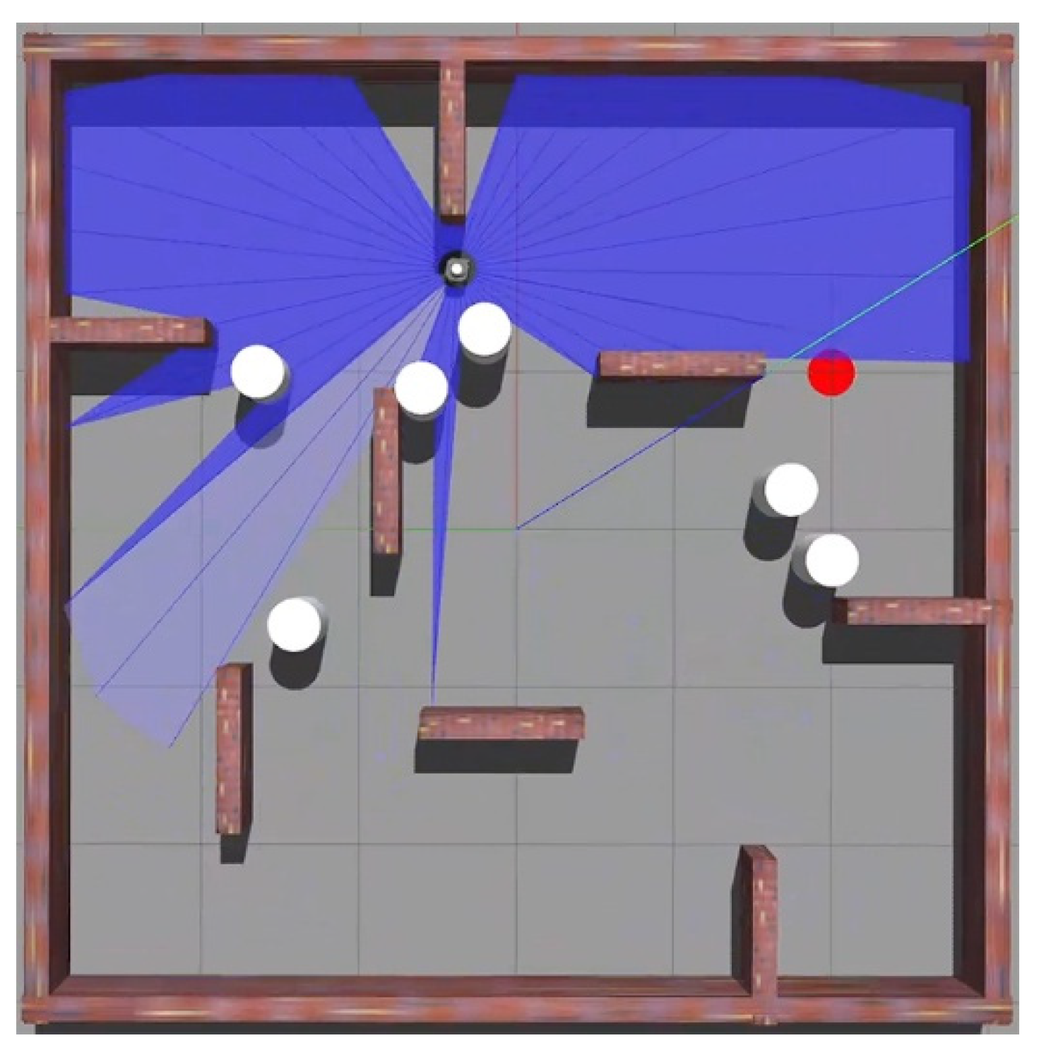
Figure 3.
Figure 3. Three assessment environments of varying difficulty, including (a) a simple environment, (b) a medium-difficulty environment, and (c) a difficult environment.
Figure 3.
Figure 3. Three assessment environments of varying difficulty, including (a) a simple environment, (b) a medium-difficulty environment, and (c) a difficult environment.
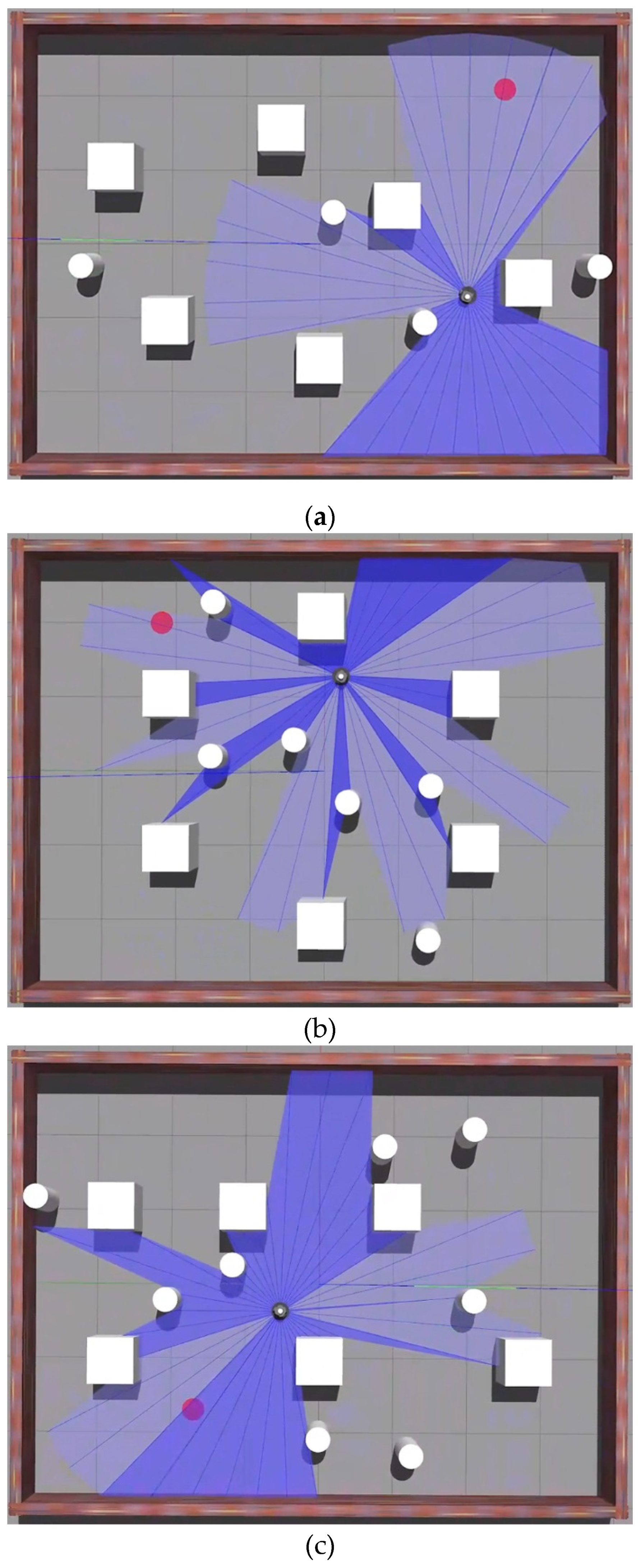
Figure 4.
Figure 4. Test results of DDPG, TD3, SAC, and ACR-TD3 in three environments of varying difficulty levels.
Figure 4.
Figure 4. Test results of DDPG, TD3, SAC, and ACR-TD3 in three environments of varying difficulty levels.
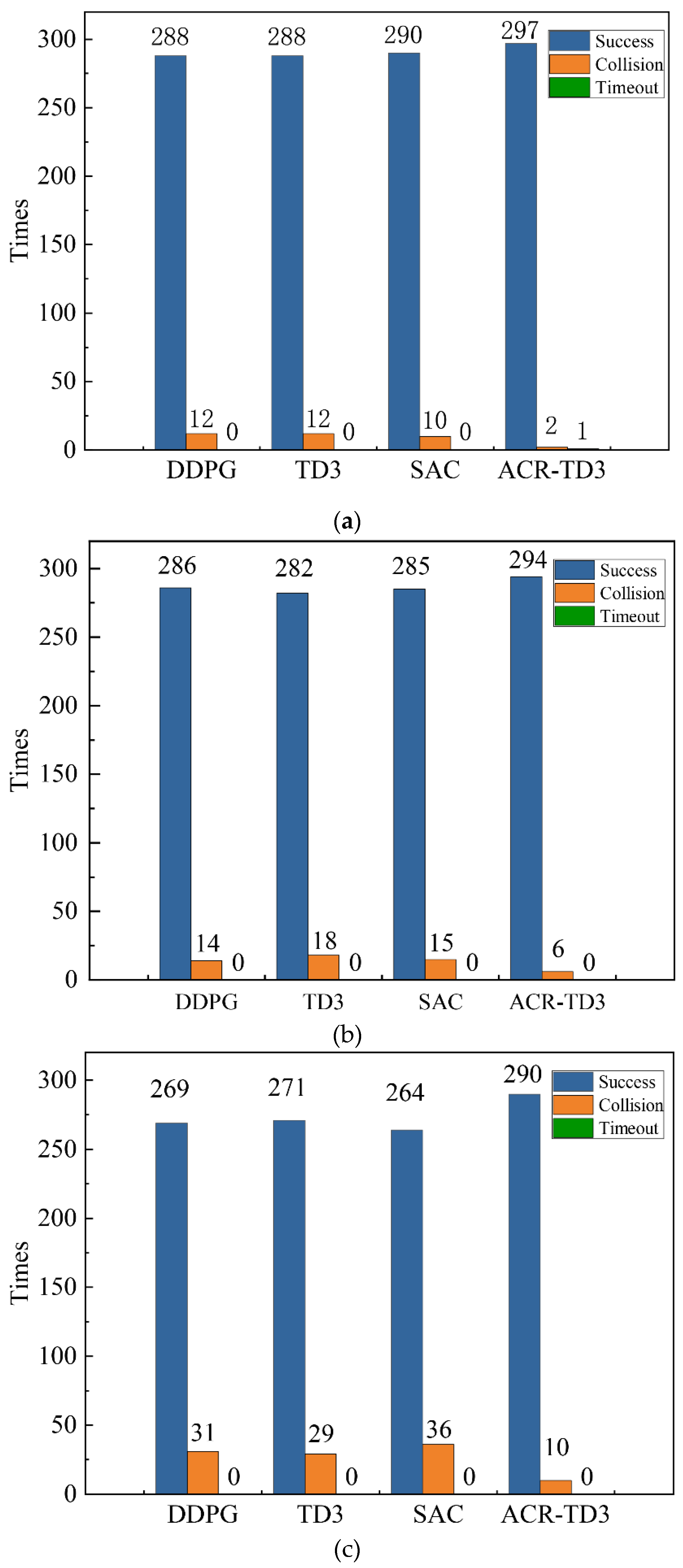

Table 1.
Network training parameters for ACR-TD3.
| Parameter | Value |
| Learning Rate | 0.0005 |
| Discount Factor | 0.97 |
| Soft Target Update Parameter | 0.001 |
| Batch Size | 256 |
| Buffer Size | 2e6 |
Table 2.
Comparison of model navigation success rates.
| Method | Env1 | Env2 | Env3 |
| DDPG | 96.00% | 95.33% | 89.67% |
| TD3 | 96.00% | 94.00% | 90.33% |
| SAC | 96.67% | 95.00% | 88.00% |
| ACR-TD3 | 99.00% | 98.00% | 96.67% |
Table 3.
Comparison of model trajectory lengths.
| Method | Env1 | Env2 | Env3 |
| DDPG | 4.476 | 4.553 | 4.785 |
| TD3 | 4.531 | 4.557 | 4.768 |
| SAC | 4.508 | 4.989 | 5.014 |
| ACR-TD3 | 4.307 | 4.452 | 4.547 |
Disclaimer/Publisher’s Note: The statements, opinions and data contained in all publications are solely those of the individual author(s) and contributor(s) and not of MDPI and/or the editor(s). MDPI and/or the editor(s) disclaim responsibility for any injury to people or property resulting from any ideas, methods, instructions or products referred to in the content. |
© 2025 by the authors. Licensee MDPI, Basel, Switzerland. This article is an open access article distributed under the terms and conditions of the Creative Commons Attribution (CC BY) license (http://creativecommons.org/licenses/by/4.0/).
Copyright: This open access article is published under a Creative Commons CC BY 4.0 license, which permit the free download, distribution, and reuse, provided that the author and preprint are cited in any reuse.


