
Submitted:
16 December 2024
Posted:
17 December 2024
You are already at the latest version
Abstract
Imaginary coquaternions cℍ can be represented by matrices of negative feedback N^-, positive feedback P^+ and reciprocal links R^± . Added environmental element E^± endows biologic systems with the structure of cℍ module. Although cℍ representation links base patterns with geometric structure of pseudo-Euclidean R_2^4 space, unknown physiologic aspects of relationships between base elements may add new functional features to the structure of a functional module. Another question is whether achieving and remaining in the equilibrium state provides stability of a biologic system. Considering the property of a biologic system to return deviated conditions to the equilibrium, the system of ordinary differential equations describing behavior of a mechanical pendulum was modified and used as a basic tool to find the answers. The obtained results show that in evolving systems the regulatory patterns are organized in a sequence NPRN of base elements allowing the system to perform the high amount of the consuming energy functions. In order to keep dissipating energy at the same level the system bifurcates and finalizes its regulatory cycle in R^± by splitting P^+ after which the next cycle may begin. Obtained flows are continuous pathways not interfering with equilibrium states, thus providing a homeostasis mechanism with nonequilibrium dynamics. Functional transformations reflect changes in the geometry and metric index of coquaternion. Related coquaternion dynamics shows transformation of hyperbolic hyperboloid to the closed surface, which is the fusion of the portions of hyperbolic hyperboloid and two spheres.
Keywords:
Coquaternion kinematics
; Lie algebra
; negative feedback
; positive feedback
; reciprocal links
; functional stability of biologic system
; non linear systems
; non equilibrium dynamics
; homeostasis
1. Introduction
The notion of a biologic system (BS) has a broad meaning. In this paper it will be used regarding biologic units, which are morphologically separable and functionally stable as reproducible elements. Thus, a notion of a biologic system can be applied to biological cells, organs and functional systems such as cardiovascular, endocrine, gastrointestinal, etc. composed from the previously determined elements [1,2,3].
At each of these functional (hierarchical) levels negative feedback , positive feedback and reciprocal links () have been observed and used as the functional patterns formalized from feedback circuits, regulating functions of two morphologic elements, subsystems, united in two-element biologic systems. Expressed in a matrix form represent basis elements of a Lie algebra of a special linear group and imaginary (vector) basis of coquaternions cℍ [3,4,5,6] (Figure 1).
represent basis elements of a Lie algebra of a special linear group. These matrices are also imaginary basis of coquaternions.
Coquaternions and split-quaternions are synonyms. Term coquaternion will be used after Cockle, the author who discovered and named this algebraic structure [7]. If the identity element of coquaternion is considered as an environmental regulatory pattern modulating functions of biologic systems, the four basis elements of coquaternion will represent the full set of four base regulatory patterns of a biologic system. Closed algebraic structure of cℍ implies that a BS has a property to be also closed under the physiologic compositions of the base elements. Based on this correspondence, it is assumed that coquaternions represent a functional module of a biologic system as a uniform regulatory structure of biologic cells, organs and functional systems [8].
Only a few data imply the existence of functional links between elements. The character of metabolic chains within biological cells have led some authors to suggest that negative feedback might provide some additional energy to activate biochemical reactions required for positive feedback function [9]. It could also be confirmed based on the well known physiologic interactions between organs such as a second stage of delivery when active contractions of the uterus increase the amount of the released hormone oxytocin, which by positive feedback increases the strength of the uterus contractions, that, in turn further increase amount of oxytocin and so on; Negative feedback mechanism along wouldn’t be able to do the delivery. Bowel movements and rectal emptying as well as sexual intercourse are explicit examples demonstrating that provides qualitatively different system’s actions and require more energy compared to the [10,11]. There is no data indicating functional links between and other base elements. Finding relations between base patterns may help to explain mechanisms of differentiation and integration of biologic systems and clarify the role of coquaternions in forming the structure of a functional module.
2. A Mechanical Pendulum as a Model of Functional Relationships Between Base Elements of a Biologic System
A functional structure of base elements is better understood through the phase portraits of ordinary differential equations (ODE). Linear dynamical models of the base patterns of biologic systems provide a good approximation of feedback circuits. Schematic descriptions of feedback circuits as two-element graphs are still considered the basic tools for understanding the physiology of these regulatory mechanisms.
Feedback responses reflect the ability of a biologic system to return the deviated states back to equilibrium. Equilibrium conditions are known as physiologic constants such as normal heart beats, blood pressure, concentration of electrolytes, hormones, glucose in the blood, etc. Achieving and maintaining equilibrium as one of the goals of being disturbed systems usually determine the modeling features to explain system’s behavior and viability [12,13].
Biologic systems are dissipative structures. It means that there is always some amount of energy accompanied by metabolic processes in the form of heat, molecular structures, etc., which cannot be reutilized further by a system. Therefore functional dynamics of biologic systems including the achieving of equilibrium states presumes that the amount of energy needed for synthesizing a biologic matter must include not only the portion, which will be conserved in the created biologic elements, but also the amount equal to the dissipated component. In other words, the functional outcome of synthesized biologic cells, tissues, organs must outweigh the system’s functional decline up to the destruction of morphologic elements as a result of natural physical decay [14]. Physical environment and metabolism itself irreversibly destroy biologic matter; only involved in a reproductive cycle biologic cells provide individual and long-term survival of biologic tissues, organs and whole organisms. Therefore, functional stability of biologic systems is not related to the achieving and keeping static conditions classically determined as equilibrium states, but a dynamical process prompting permanent input of energy to compensate for natural functional decline and, at least, maintain already achieved functionality. The Cell Renewal Cycle (CRC) (not to be confused with cell mitotic cycle) consisting of the oppositely directed cell destruction and cell proliferation processes is a simplest physiologic model of metabolism, which generalizes the notion of homeostasis mechanisms as “chasing” the keep increasing levels of thresholds of equilibrium states [8].
The Gibbs equation is a simplest expression of the fact that, if entropy of the system is an increasing in time function, energy flow into the system should also be increasing in time to compensate for growing entropy S and keep inner energy of the system at the functional level. This supports the above statements.
There are four types of phase portraits of linear autonomous systems (Jordan normal forms and Poincare diagram) based on the characters of the fixed (equilibrium) points [15,16]. We will consider “naïve” structural stability of the system based on this classification. Originally is represented by a neutrally stable structure [3]. Its phase portrait is circular trajectories surrounding equilibrium point, which is also a phase trajectory. Small disturbances will change the character of trajectories, which may converge towards equilibrium point or diverge from it. It is natural to consider the disturbing factor as some environmental forces, which will be represented by a diagonal (environment) matrix added to the matrix of (Figure 2). The obtained autonomous systems will show opposite dynamics depending on the signs of the elements of . In this case, classically stable systems shown as converging to the equilibrium phase trajectories eventually will demonstrate no changes in the systems conditions after achieving the equilibrium states, hence, if staying in these states the systems will die due to increasing entropy. So an equilibrium condition can be interpreted as the state eventually leading the system to death. Life is always the fluctuations around equilibrium; this is analogous to a cardiac function measured through the electrical activity of the heart - straight line (asystole) means cardiac arrest, which is stop of functioning. On the other hand, unstable systems, which are structurally stable, with diverging dynamics are also not viable because the necessity to increase functional output will eventually meet functional and morphologic incompetence of the system.
and patterns correspond to a saddle and are structurally stable regulatory systems. They contain stable and unstable manifolds [15,17]. Matrices of these operators relative to the same basis determine topologically equivalent systems, which can be obtained by orthogonal transformations or rotations of the plane around the axis through the equilibrium point at 45 deg. Further it will be shown that the same matrix of reciprocal links , but related to a different operator is obtained by similarity transformation of matrix of positive feedback ; it changes the basis of the space of biologic variables relative to which matrices are expressed.
If a biologic system has the property to return deviated states to the equilibrium, then some inner forces must exist inside the system, which are assumed to be operated through the activation of the base, elements of the system’s internal structure. To describe this mechanism, consider a simple mechanical pendulum modeling a biologic system dynamics. Displacement of the mass from the lowest position, equilibrium, will increase potential energy of the system, which after releasing the mass will cause its movement towards equilibrium, increasing kinetic and decreasing potential energy of this system. After reaching the equilibrium all accumulated by the mass’s displacement potential energy will be transformed into kinetic energy, which reaches its maximum level. If the friction is not considered, the mass will perform small swings around equilibrium with the same amplitude. The swings will cause transformations of potential and kinetic energy to one another until swings continue [18,19]. A simple pendulum with normalized parameters is described by a classic second order differential equation
equivalent to the system of two ODEs whose variables, -displacement, - velocity, which for more accuracy in application to a biologic system is considered with some parameters
The system has three equilibrium points. At zero point its phase portrait is a center which is concentric circles. A matrix responsible for this phase portrait is a skew diagonal matrix . Without friction and external forces, the simple pendulum will perform small swings and its dynamics expression is analogues to the (N-) pattern (Figure 3). The closed trajectories correspond to the energy levels of the system. Total energy of the system .
Behavior of the pendulum is also well described when friction and external forces are added as factors modifying its behavior [14,15].
For our purposes we will consider an environmental factor added to the system (2) in the form of diagonal matrix with the same signs of coefficients of ;
Parameter determining friction in classical models () can also provide acceleration (), and of the first equation should have concomitant action on variable because of the same signs of coefficients of .
For simplicity the system (3) will be considered with the normalized parameters. It also will help to understand and visualize relationships between patterns. The system (3) with normalized parameters has also three equilibrium points: (Figure 4).
Matrix of the normalized and linearized system (3) is
At it is presented as a sum of unsteady stellar node matrix of environment and negative feedback pattern presented by . The nature of patterns is determined by the signs of entries and determinants of the matrices, not magnitudes of entries, so depending on the context the sign marks as only matrices entries will be used.
Behavior of the system (3) as diverging from equilibrium shows increase of the total energy supplied by the environment. Physiologic sense of and base elements acting together depends on the considered time scale. In relatively large periods of time increasing the total energy of the system can be related to domination of anabolic processes over catabolic ones when morphologic structures are capable to support the system’s function either by proliferation or hyperplasia. For short time intervals it can be interpreted as rapid movements of the states of the system dictated by the necessity to accelerate metabolism. The behavior, corresponding to the trajectories of unstable node is not the only one, which potentially could experience the normal system; a<0 and d<0 cause the system to behave as a stable node when the states are converging to the equilibrium. This functional pattern is also physiologically acceptable, for instance, during physical decline, illnesses, etc., causing exhaustion of energy of the system, and, if not treated, the death (see Figure 2). For our purposes we will consider a developing system, which accumulates potential energy in the form of growing and multiplying morphologic elements.
When the energy of the pendulum continues to increase, the character of the movements changes from swings to rotations, which are described by equations of upside down pendulum. It occurs when the increasing energy overcomes some structural threshold of the pendulum. At the points when swings transform to rotations the system (3) bifurcates and acquires new behavior and a regulatory mechanism. These points are crucial for the system’s behavior. In the phase portrait they correspond to the homoclinic trajectories, which are two separatrices, forming loops originated from and coming back to a saddle equilibrium point [18,20] (Figure 5).
As it was mentioned above (3) has two other, besides zero, equilibrium points. These points at and correspond to saddles.
The part of the system related to the matrix (4) not affected by environment has a non- degenerate critical points at obtained from , which are thresholds of potential energy when transforms to . Corresponding phase curves will change the curvatures from convex to concave. From now on the convenient way to describe system’s development is from the top, non steady, equilibrium position of the pendulum.
A cubic function will express gradient of potential energy of upside down pendulum described by differential equation where the right side of the equation (1) is considered with positive sign and (2) and (3) will have c<0. New equilibrium point for convenience will be at zero coordinate. Corresponding (1’), (2’) and (3’) systems with positive values of the parameters are (Figure 6.)
Linearized system (2’) at is a saddle. The cubic expression for the gradient of potential energy of the system will determine closed phase trajectories because of the prevalence of when (potential energy of the system) continues to increase. At obtained from curvatures of the closed curve will change according to the hyperbolic and elliptic structures of the curve, which will replace each other (see Figure 5).
Behavior of the system without interference of the environmental factors (2’) shows that after moving to a higher energy level the system’s conditions may oscillate confining two phase portraits of . Metabolic pathways, shown as negative feedback trajectory surrounding two other negative feedback curves, require more energy than each of two banded together subsystems. The surrounding two systems loop is separated from these systems by homoclinic trajectories, which are separatrices, originated from the hyperbolic equilibrium point (see Figure 5). Related transformation mechanisms reflect a special property of a biologic system to activate its inner energy sources and switch from the lower energy pattern to the higher energy consuming function and further on to . This property expressed through the cubic function is termed in this work a biogenic active property (BAP) of a biologic system.
Environment substantially changes the character of phase trajectories of the system. When normalized system (3’) becomes and it is easy to see that the unstable structure of the environment transforms closed phase trajectories of negative feedback surrounding the other two curves into the unstable node. Action of environment added to the system (2’) will make it diverge as in the case when the system is regulated by and patterns before it bifurcates. Phase portrait (2’) and (3’) also shows that closed trajectories originated from and confining two subsystems become divergent. If this regulatory mechanism continues developing without structural changes, it eventually will destroy the system (Figure 7).
It seems that nature has found the means to solve this problem, first, by splitting operator and the space of variables into two parts and then integrating the obtained components. Eigenvectors of two one dimensional subspaces after splitting have become expressed relative to the new basis, which are combinations of the previous basis elements. The way the separation of the elements is obtained makes the analytical description as well as a physiologic process of differentiation not trivial. Moreover, it would also require reorganizing morphologic and functional elements of the system. The process of morphologic adaptation, in fact, begins simultaneously with functional changes of the system, so by the time when qualitative changes have occurred morphologic elements will be ready to adapt its structure to the upcoming events.
transforms to equivalent pattern by conjugation diffeomorphism h: ; Importance of this transformation for the system’s stability lies in the property of the obtained matrix to have a diagonal view with real elements (eigenvalues), thus to be presented as a direct sum of two operators acting on one-dimensional subspaces. Moreover, similarity transformation changes the initial basis to relative to which matrix of is expressed. The new basis is a linear combination of basis elements: , . Combinations of the basis elements and opposite signs of eigenvalues make representing subsystems act as separate units with opposed functionality. Matrix representing the reciprocal links pattern is a direct sum of two operators in the space of biologic variables , which is a direct sum of two one dimensional subspaces and spanned by the new basis elements . As a result the system can hold total energy, which becomes distributed between two relatively simpler independent subsystems. Important property of is providing the “special” functional links between vectors satisfying , where is a constant. Corresponding hyperbolas are trajectories of the same energy levels.
What the pendulum model implies is that accumulated energy “helps to choose” the right regulatory mechanism (functional pattern) to manage the current system’s condition. Thus, the properties of four base elements organized in a sequence will determine the global functional structure and dynamics of the system depending on the available energy. That functional patterns can be organized in a sequence, in fact, reflects the global tendency of the system to use increasing amounts of energy to maintain continuity of metabolism and stability of the performing functions. and related mechanisms in the pendulum model were modified by environmental factors .
3. The Structure of the Base Functional Patterns Determines Nonequilibrium Dynamics of Biologic Systems
Base functional elements of the system with the related to the environment pattern present basis elements of coquaternions (coquaternions’ ring) whose elements span pseudo-Euclidean 4-space over ℝ. Heterogeneity of the space determined by the structural differences of the base elements, in turn, determines the character of relationships between variables and . and patterns determining changes in the system’s conditions cannot split and variables. In other words, the well-known negative and positive feedback circuits can’t manage involved in these mechanisms subsystems separately. If the current condition of one subsystem changes, the condition of another subsystem will also change, obeying the feedback action of the first subsystems. Each condition of the system is a pair considered as a whole character. Only virtually they are separate, independently acting characters. For instance, pituitary and thyroid glands are anatomically separate organs with their own functions. Roughly pituitary produces thyroid stimulating hormone TSH and thyroid gland- T3 and T4 hormones. Any changes in the concentration of thyroid hormones will evoke negative feedback response of the pituitary and change of concentration of TSH. In turn, it will stimulate or inhibit actions of the thyroid. These organs act as the whole functional unit. None of the known physiologic mechanisms makes them act independently. The same is true regarding the strength of the uterus contractions and the posterior pituitary responsible for the release of oxytocin during the labor. Only together these organs are capable to provide the uterus with the contractile forces required for delivery, thus to perform the system’s action generated and regulated by a positive feedback mechanism.
This simple from the first glance observation lies on the property of and ( and patterns, respectively) to be the matrices of complex and split-complex structures on the spaces of variables x and operators and determining phase flows as one parameter groups of diffeomorphisms ; . Decomplexification allows these structures to be presented as direct sums of subspaces and operators. This construction, in fact, doubles dimensionality of the real spaces where physiologic variables and operators are being measured.
and are direct sums of the spaces of splitors [8], where and are the spaces for and patterns and environmental spaces and for pattern. Now the spaces of physiologic variables with the environment can be considered as the whole units. The existence of the environmental component becomes a natural complement to and resulted in doubling of dimensionalities of the spaces. It was an environmental element formally added to occupy the real parts of the obtained subspace.
, are complex and split-complex matrices with respect to and bases of operators and , respectively, where , and , ; . , , are matrices corresponding to environment and negative feedback and positive feedback, respectively. These structures can be written in the following forms: for complex matrices; for split- complex matrices.
As it was mentioned above and are irreducible second order matrices relative to the standard basis.
Split- complex matrix has its conjugate , and this transformation makes regulatory structure reducible to one dimensional operators and whose eigenvalues are of opposite sign. These operators form a direct sum , which makes them act separately on one dimensional invariant subspaces , ; ⊕ and also on pairs of functionally related variables satisfying (see Figure 1). These spaces are over ℝ. , , ⊕. The new basis elements of and are , , respectively.
The matrix of a complex structure also has its conjugate as a diagonal matrix with complex eigenvalues . It is a direct sum of two complex operators , acting on complex eigenvectors of one dimensional invariant subspaces associated with the new complex basis vectors along coordinate axes and : , ; ⊕ . These spaces are over . , , ⊕ .
New basis for and is , . These are not the only combinations acceptable for the new basis elements from . For instance, another combinations can be , Important, that real parts are from .
The spaces are disjunctive, satisfying the condition , so that a direct sum is a four dimensional space and linear combinations of the vectors from this space allow considering the sums and , which for and operators in a matrix form reads
It is obvious that the initial space has become split into the two functionally opposite subspaces regulated by and )
For the real form of , , there is a conjugation matrix C∈, which transforms it to a skew diagonal form =.
Now it is easy to see that the obtained negative feedback pattern is presented by compositions of elements, which are integrated from the simpler patterns. This construction defines hierarchy between blocks considered as the single not structured regulatory elements operating on a pair of variables and elements of the blocks providing differentiated actions on single variables. Thus, the matrix blocks transform pairs of variables as a whole element and after that each variable is managed separately as a discrete element depending on the inner structure of the considered block.
works as pattern of negative feedback whose elements are the skew diagonal unit matrices organized in 2x2 blocks with opposite entries. will make the related 4-vector to be involved in the next cycle. The structure of two inner functional cycles and related to the split elements will be finalized in the formation of two orthogonal coquaternions.
This construction also determines evolution of the systems in two different directions: by forming the structural complexes from the existing elements, and, at the same time, splitting the element into congruent simpler components.
Actions of environment (system 3’) will provide evolution of the system’s states as diverging phase trajectories result in the following sequence of regulatory mechanisms: center, focus (unsteady node), then, saddle with homoclinic trajectories included.
The images of two unsteady nodes bounded by closed curves (or curves of unsteady nodes in case of environmental actions) correspond to the subsystems which would be stemmed and developed after the bifurcation. The neighborhood of a saddle point presupposes the formation of these subsystems. The four separatrices virtually split the system and demonstrate equal contributions of two subsystems, elliptic and hyperbolic, in the evolution of the whole system. Right upper separatrix shows simultaneous increase of potential and kinetic energies (and variables) moving the system’s conditions to the higher functional level. The phase portrait of the system after the splitting also corresponds to the saddle equivalent to the image of rotated on 45 degrees counterclockwise (see Figure 1). Two one dimensional subsystems obtained after the transformation will be defined by new variables, which are obtained as linear combinations of the previous ones, . , as the new basis vectors are orthogonal to each other as eigenvectors of one dimensional subspaces. Considered as new variables and with their velocities added to the system as variables and , the formed subsystems will be relatively independent and regulated by orthogonal operators and . Obtained and systems are similar to the initial system as potential and kinetic energy variables. Two connected by the linking diffeomorphisms subsystems and also present a system . As a whole functional structure it will follow the same nonequilibrium changes as the initial system. Thus, closed regulatory cycle = is obtained when after the splitting two subsystems hold the wholeness of the system’s structure due to integrating the subsystems reciprocal links (diffeomorphisms). The first originates from the last pattern of the previous cycle, so it inherits the basis relative to which the corresponding and following matrices are expressed until splits again. From the split points there are two directions of how the progeny system will develop – two split subsystems can act as independent units (systems) and as an integrated system. As a system it can develop independently following previously described mechanisms of transformations. Physiologically the first ones provide a biologic system with the mechanism of differentiation, while the latter with the integration.
4. Coquaternion Module Dynamics in Transformations of the Base Patterns
All coquaternion basis elements are involved in a chain as regulatory patterns. Scalar element added to each part provides smooth transformation or transition of the patterns depending on thresholds and a specific character of the development. These patterns may form combinations to each other. For example, a combination of pure and is able to deform related diffeomorphisms, not changing its hyperbolic nature. Physiologically, most probably it would be preceded by and involved in regulations especially in developing organisms after the system bifurcates. is a diffeomorphism linking neighbors, being split, functional systems in a manner preserving the dot product of these systems . It determines horizontal relations between two, the newly born developing characters. On the other hand, the two subsystems determining these characters pursue their own coquaternion cycles, so they develop vertically, inside the system. Thus, evolved from the initial system a functional module determines a two- level hierarchy, or two orthogonal hypersurfaces presented by coquaternions. Formally speaking the obtained two pathways organized as orthogonal circles form a torus (algebraic torus) where each circle trajectory is a sequence of coquaternion elements.
Geometry of coquaternions is related to space and its indefinite metric structure is determined by the algebra of the basis elements. When the basis is represented by the above discussed matrices , the matrix determinants, , will determine diagonal elements of the Gram matrix of quadratic form and (2,2) metric index of the 4-space of coquaternions [5,6,21]. For the given coquaternion the scalar product on one-forms is a quadratic form . The value of the quadratic form is determined by one-forms and they won’t change the metric index. Changing values of one-forms will only “deform” geometry of the surfaces leaving the metric index the same. Thus determinants of the matrices of the basis elements will determine the main structural characteristics of the functional module of the normal biologic system.
No other than cℍ structure with the basis obtained from the three forms of feedback exist, if maintaining the wholeness of biologic systems’ structure is determined, first, by splitting and, second, by integration of split components when the system’s conditions reach some functional thresholds during development. Maintaining normal systems structure is functionally equal to the system’s evolution in its narrow sense considered as a process escaping equilibrium states and providing functional stability and structural steadiness through the transformations of the base regulatory patterns. Closed cℍ structure as an algebraic noncommutative ring confirms or suggests closed structure of relationships among the base elements. Split-octonions as the next algebraic construction loses the distributive property of its elements and becomes unstable as a functional unit in terms of reproductivity of its regulatory structure in biologic systems. So, four dimensional spaces provide structural limits to present a functional module as invariant regulatory structure of biologic systems.
and (in parentheses are formal cℍ basis elements) will determine orthogonal coordinates and geometric image of hyperbolic hyperboloid (hyperboloid of one sheet). It is expected that system’s dynamics will demonstrate similar images in (, ) and , planes because of the automorphism of ) and operators determining closed trajectories obtained from the sections of hyperbolic hyperboloid perpendicular to axis. Sections through will determine non degenerate critical points as points on the circle where hyperbolic hyperboloid transforms to the sphere. Closed trajectories related to the pendulum rotations will be projections of the three dimensional image onto the plane of variables. Each closed surface corresponds to a certain energy level as the value of associated quadratic form whose metric will undergo transformation from to . This can be seen from the linearized matrix having alternating determinant values around critical points, therefore making changes in the metric index (Figure 8).
Thus, cubic function makes unbounded coquaternion surfaces bounded and closed by portions of the spheres. It demonstrates additional features of biogenic active properties of biologic systems. The system becomes capable to confine the energy at a certain conditionally stable level and act as an autonomous system also maintaining activities of two other systems. It means that the coquaternion module contains integrative properties in its structure allowing the obtained after splitting subsystems to be regulated as a whole unit by (closed trajectory).
On the other hand, action of environment can make the surface of hyperbolic hyperboloid diverge markedly from the zero point, which must suggest the necessity of earlier system transformations including splitting (Figure 9). Metric transformations can be a normal part of the system’s behavior allowing the system to maintain its functionality adequate to the available energy, preventing system’s destruction. When nonequilibrium states are considered as normal system’s dynamics, actions of the environment will keep the system moving to the higher functional levels through the thresholds when regulatory mechanisms switch to apoptosis and cell proliferation and eventually to the reproduction of the whole organisms.
5. Results
It is implied that in order to maintain continuity of metabolism, the sequence of transformations of the base elements as regulating metabolism patterns must be finalized in a “special” regulatory pattern, which will create a new germ,- two separate characters as autonomous systems each potent for the development and at the same time congruent to be integrated into another system. This pattern is presented by a reciprocal operator, which is a direct sum of two operators acting on one- dimensional subspaces. Similarity transformation by which this pattern is obtained splits regulatory structure of the new system onto two relatively independent mechanisms dividing the system into two subsystems. This provides a biologic system with continuity of functional regulatory mechanisms by creating separable inner morphologic elements presented by two subsystems.
Continuity of biochemical reactions through transformations of PNR base physiologic patterns is a substantial feature maintaining viability of biologic systems, thus, determining homeostasis mechanisms. Considering metabolism as a process of obtaining energy for chemical transformations and changes of the system’s conditions homeostasis will make metabolic flows continuous and “avoiding” equilibrium states. On cellular and organ level homeostasis is provided by continuity of symmetric and asymmetric cell divisions [8,22] involved in CRC.
Because of splitting of the initial system into two subsystems and identifying split elements (subsystems) with the progenitor system, the way the uniform structure, a biologic system, is obtained also determines a functional hierarchy between the systems. There are only four pieces of one dimensional manifolds (saddle) associated with coordinate axes where the split systems are totally independent. The areas between them are filled with the hyperbolic curves of “reciprocal” diffeomorphisms between subsystems satisfying Each hyperbolic trajectory lies in a certain energy level of the system. The character of the trajectories also shows mutual transformations of kinetic and potential energy of the components. Reciprocal links, in fact, is a mechanism of integration of biologic systems that originated from common roots before splitting. Demonstrative example is clot-formation and clot-degradation subsystems regulating viscosity of the blood. Function of each subsystem is provided by cascades of biochemical reactions acting in reciprocal manner: when clot-formation subsystem is active making viscosity of the blood high enough for blocking the arteries by forming clots, the clot-degradation subsystem will act inversely to compensate functions of the overactive clot formation system and prevent harmful consequences of not keeping the rheology of the blood within normal physiologic ranges.
Coquaternion structure is a logical sequence of the four base elements organized in a functional cycle forming the vertical hierarchy of developing systems. Closed algebraic structure of coquaternions implies wholeness of functional relationships between base regulatory elements forming the structure of a functional module of biologic systems.
Obtained results can be summarized as follows: the strategy of biologic systemogenesis is aimed at the formation of discrete units with the highly integrative properties.
6. Discussion
A biologic system is a dissipative structure and equilibrium state, when conditions are static, not changing in time, and might not characterize the system’s stability and viability. A viable system dynamics is always fluctuations (!) of the conditions around equilibrium. Only in a large scale of measured quantities fluctuations are not detectable, therefore conditions are considered stable, not changing in time characters. Moreover, biologic systems have some stages of maturation that should displace the normal ranges of physiologic constants, and the states initially considered normal when the system is immature are becoming abnormal and out of normal ranges with the aging. The cell renewal cycle (CRC), which, in fact, should be considered as the System Renewal Cycle (SRC) validates this statement demonstrating continuous renewal processes of biological cells, tissues and organs by renovating becoming “old” and malfunctioning systems.
The Gibbs equation formally implies dissipative property of biologic objects by including entropy in the equation, which would increase the total amount of energy required for the system to maintain its structure and function. Permanently growing entropy increases the system’s malfunction that, in turn, will require an increasing amount of energy input to maintain the functionality.
In order to describe “nonequilibrium” behavior of biologic systems, the simple physical analog, a mechanical pendulum, has been considered as a model.
Function of mechanical pendulum is determined by potential energy of the displaced from equilibrium mass. Until additional energy is not added to the pendulum, it will perform simple swings around low equilibrium position. When the pendulum attains amount of energy overweighing its structural threshold the swings change to rotations. Behavioral patterns described by ODE will demonstrate two qualitatively different regulatory mechanisms determined by mutual transformations of potential and kinetic energy and the total amount remaining conserved. Corresponding to the pendulum dynamics phase trajectories are center and saddle. These events occur according to the Hamiltonian mechanics which in small mimics biologic processes.
Well known physiologic property of biologic systems to move displaced conditions to the normal, equilibrium states was the determining factor in formulating the modeling conditions. Negative and positive feedback circuits observed in biologic systems have been found to be similar with the pendulum mechanisms determining behavior. If additional energy is added to the pendulum, it causes transformations of phase trajectories from center to the saddle and changes the character of the pendulum movements from swings to rotations.
Unlike mechanical systems, a biologic system is able to activate its inner sources and switch regulatory mechanisms from to . This feature was named in this work a biogenic active property (BAP) of a biologic system and the cubic function has provided this modeling feature. Environmental operator in the form of a diagonal (identity) matrix was added to the system of ODE. Energy levels become not quantized as in the case of “conditionally” steady operator of negative feedback. Environmental operator makes transformations of the system’s conditions to be the smooth diverging from equilibrium phase trajectories moving the system’s conditions towards a functional threshold.
Nonlinear element in the form of cubic function is a key in determining the first node-saddle bifurcation and further dynamics related to the formation of closed energy trajectory confining two curves. Dominance of the cubic summand during increase of potential energy changes regulatory patterns from to , which returns back when potential energy decreases and kinetic energy component becomes the leading cause in changing the character of movements and keeping the trajectory closed. Thus the curve, being initially hyperbolic, becomes elliptic, and then changes its shape again when approaching saddle equilibrium. The changes continue in the opposite direction until the curve becomes closed. Closed trajectory corresponding to the constant energy level becomes diverging from the saddle equilibrium in the form of an unstable node when an identity matrix is added making the environment a factor providing growth of the total energy of the system.
Similarity transformation preserves the matrix determinant that suggests the operation as requiring minimum energy. Hence, by the time node-saddle bifurcation occurs, the obtained regulatory pattern would simultaneously transform to and both under the actions of the environment would evolve further following diverging trajectories. Similarity transformation resulted in conjugation diffeomorphism splits the operator of positive feedback into a direct sum of two operators of reciprocal links. Physiologic importance of this transformation lies in the distribution of the conserved total energy between two subsystems and the property of obtained regulatory structure to manage each one dimensional subsystem independently. On the other hand, the structure of allows the new obtained variables to be regulated following reciprocal feedback between them such that to keep the integrated energy level on the constant level. Conjugating diffeomorphism provides further development in two simultaneously evolving directions- vertically by pursuing differentiation of obtained morphologic elements and horizontally integrating differentiated elements.
Closed planar trajectories corresponding to the pendulum model will be transformed into the closed surface(s) in the case the matrices of the environment , negative feedback , positive feedback and reciprocal links will be considered as forming a basis for coquaternion representing a functional module of biologic systems. Functional structure corresponding to the closed surfaces is a fragment of dynamical changes along geodesics demonstrating equipotential conditions related to a certain constant level of the total energy of the system. Physiologically these conditions are “equilibrium” points of a constant value of the difference between anabolism and catabolism measured for conservative systems at a certain time. Equivalence of and operators provides symmetry of coordinate axes associated with quadratic form and cylindrical surface of hyperbolic hyperboloid. Its transverse sections are circles (ellipsoids) determined by conjugating and variables diffeomorphisms. A not bounded surface of a hyperbolic hyperboloid theoretically is points when catabolism dominates anabolism and quantitative difference remains at a certain level when both components increase or decrease simultaneously. So, these surfaces are equinormal points when opposite metabolic components increase or decrease simultaneously. When the sum of the absolute values of the total amount of potential and kinetic energy remains at the same level, the corresponding surface becomes equipotential and closed. Equipotential conditions must also cause fluctuations of potential and kinetic energy components whose sum will be kept at the constant level according to the parameters of the surface. To maintain the same total energy level (=closed surface) hyperbolic hyperboloid determining coquaternion metric index undergoes transformation to corresponding to the sphere and backwards until closed surface is obtained. Environment will make the closed surface sliced though. Slices will diverge from zero point. Although the environment makes systems dynamics and related trajectories divergent and unstable, morphologic structure will determine functional limits serving as thresholds when regulatory mechanisms switch the transforming system to the next stage of development unless it splits and a new cycle begins. From this directly follows that biologic systems evolve through the formation of discrete integrable units.
7. Conclusion
Understanding the nature of biologic systems through the geometry of cℍ is a new methodology in investigating biologic objects. Medical and biologic processes will become more observable by introducing cℍ as a space of algebraic elements providing biologic systems with the structure of a functional module. Further theoretical and practical investigations directed towards understanding how physiologic combinations of base regulatory elements contribute to the functional features and stability of BS may further elucidate their role in homeostasis mechanisms and in a hierarchical structure of the space of splitors.
Funding
This research received no funding.
Institutional Review Board Statement
Not applicable
Informed Consent Statement
Not applicable
Data Availability Statement
Not applicable
Conflict of Interests
The author declares no conflicts of interest
Endnotes
The materials of this paper are partially based on the author’s presentation: G.Davvydyan. “Coquaternion kinematics in homeostasis mechanisms of biologic systems”. Special session on Quaternions of Joint Mathematics Meeting held in San Francisco, California, January 3-6, 2024
References
- L. von Bertalanffy. General System Theory: Foundations, Development, Applications; George Braziller: New York, NY, USA, 1973. [Google Scholar]
- Anochin, P.K. Theory of Functional System; Science (“Nauka”): Moscow, Russia, 1980. [Google Scholar]
- Davydyan, G. Conception of Biologic System: Basis Functional Elements and Metric Properties. Journal of Complex Systems 2014, 2014, 693938. [Google Scholar] [CrossRef]
- Davydyan, G. Carcinogenesis: alterations in reciprocal interactions of normal functional structure of biologic systems. EURASIP Journal on Bioinformatics and Systems Biology, 1186. [Google Scholar]
- Pogoruy, A.; Rodrigues-Dagnino, R.M. Some algebraic and analytical properties of coquaternion algebra. Advances in Applied Clifford Algebras 2008, 20, 79–84. [Google Scholar] [CrossRef]
- Carmody, K. Circular and hyperbolic quaternions, octonions, sedionions. Applied Mathematics and Computation 1997, 84, 27–47. [Google Scholar] [CrossRef]
- Cockle, J. On Systems of Algebra involving more than one Imaginary; and on Equations of fifth Degree. The London, Edinburgh and Dublin Philisophical magazine and Journal Science 1849, 35, 434.
- Davydyan, G. Coquaternions, Metric Invariants of Biologic systems and Malignant Transformations. AppliedMath. MDPI 2023, 3, 60–87. [Google Scholar] [CrossRef]
- Ferrell James E, Jr. Feedback loops and reciprocal regulation: recurring motifs in the systems biology of the cell cycle. Current Opinion in Cell Biology 2013, 25, 679–686. [Google Scholar] [CrossRef]
- Guyton Arthur, C. Textbook of Medical Physiology. (8ed). Philadelphia: W.B. Saunders. 1991. 7216. [Google Scholar]
- Khaled A Abdel-Sater. Physiological Positive Feedback Mechanisms. Am. J. Biomed. Sci. 2011, 3, 145–155. [Google Scholar] [CrossRef]
- Reimann, S. Homeostasis and Stability. Preprint, Research Center for Interdisciplinary Studies on Structure Formation. University of Bielefeld, P.O. Box 10 01 31, 33501, Bielefeld, Germany, Dec. 18, 1996, p.1-13.
- Giuliani A; , Vici A. Stability/Flexibility: the tightly coupled homeostasis generator is at the same time the driver of change. Ann Ist Super Sanità 2024, 60, 77–80. [Google Scholar] [CrossRef]
- Vakulenko, S. Complexity and Evolution of Dissipative Systems. De Druyter, 2014. pp. 0266. [Google Scholar]
- Drazin, P.G. Nonlinear Systems. Cambridge University Press, 1992. pp. 4066. [Google Scholar]
- Arrowsmith, D.K.; Place, C.M. Ordinary Differential Equations. Chapman & Hall 1982. 0412. [Google Scholar]
- Zehnder, Z. Lectures on Dynamical Systems. European Mathematical Society, 2010. pp. 0371. [Google Scholar]
- Arnold, V.I. Mathematical Methods of Classical Mechanics. Nauka.
- Rivera-Figueroa, A.; Lima-Zempoalteca, I. Motion of a simple pendulum: a digital technology approach. International Journal of Mathematical Education in Science and Technology 2021, 52, 550–564. [Google Scholar] [CrossRef]
- Tabor, M. Chaos and Integrability in Nonlinear Dynamics. John Wiley & Sons, Inc. 1989. Pp. 364. 8272. [Google Scholar]
- Kostrikin, A.I. ; ManinYu.I. Linear Algebra and Geometry. “Nauka” 1986. p.
- Gómez-López, S.; Lerner, R.G.; Petritsch, C. Asymmetric cell division of stem and progenitor cells during homeostasis and cancer. Cellular and Molecular Life Sciences 2013. [CrossRef] [PubMed]
Figure 1.
Sketch of phase portraits of base functional elements of a biologic system and representing them real matrices
Figure 1.
Sketch of phase portraits of base functional elements of a biologic system and representing them real matrices
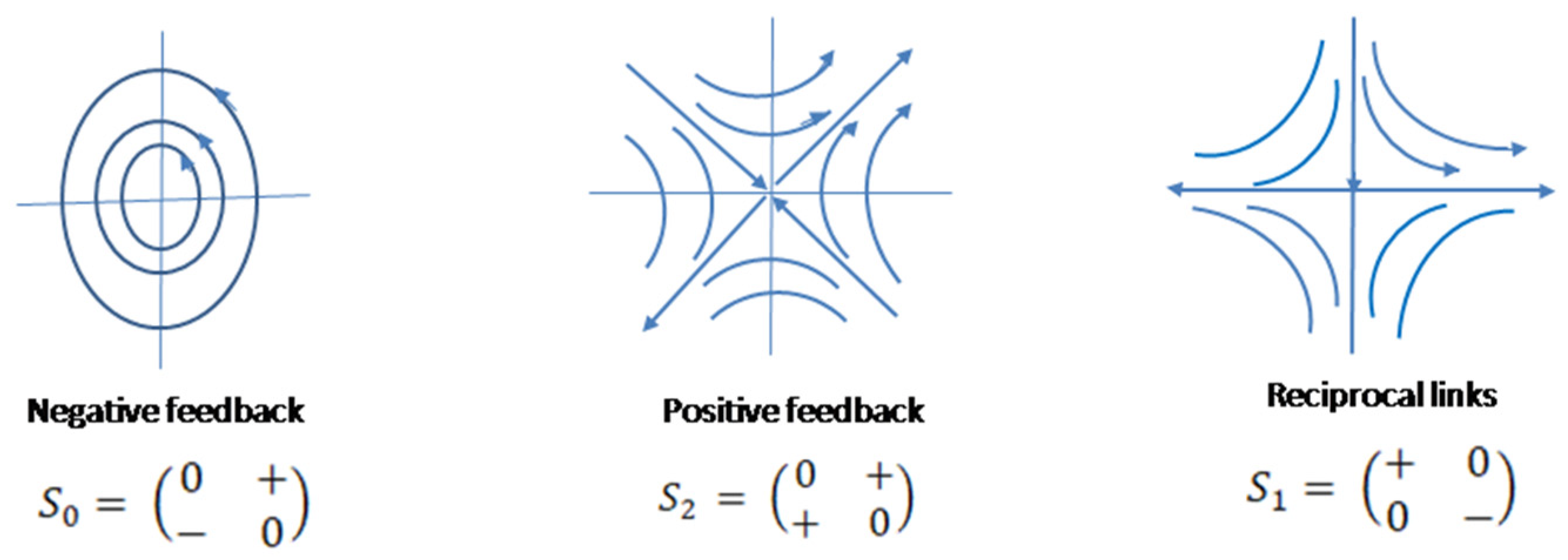
Figure 2.
Sketch of stable, neutrally stable and unstable systems. Neutrally stable systems (in the middle) are sensitive to environment and demonstrate stable (left) or unstable (right) behavior.
Figure 2.
Sketch of stable, neutrally stable and unstable systems. Neutrally stable systems (in the middle) are sensitive to environment and demonstrate stable (left) or unstable (right) behavior.
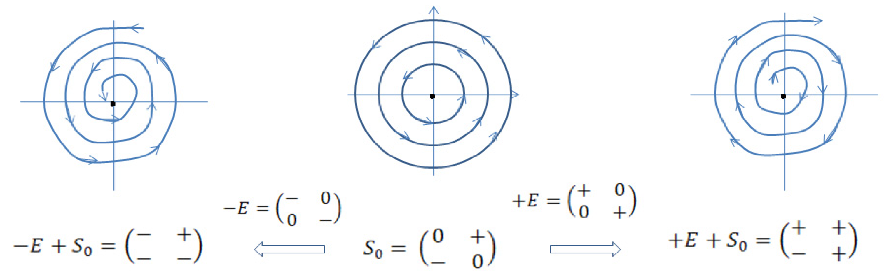
Figure 3.
Sketch of phase trajectories of small swings of mechanical pendulum Periodic pendulum movements imitate physiologic fluctuations of system’s conditions. Phase trajectories of small swings resemble biologic negative feedback mechanism.
Figure 3.
Sketch of phase trajectories of small swings of mechanical pendulum Periodic pendulum movements imitate physiologic fluctuations of system’s conditions. Phase trajectories of small swings resemble biologic negative feedback mechanism.
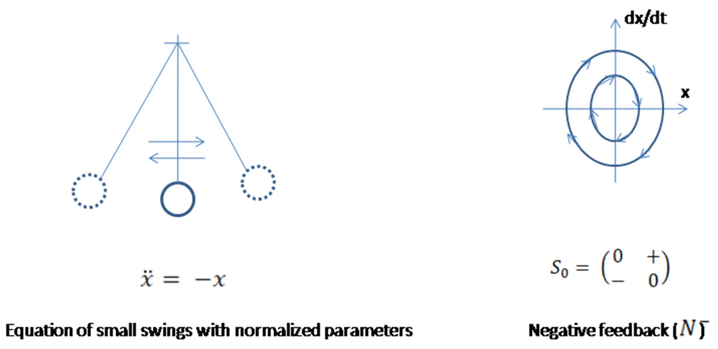
Figure 4.
Sketch of the phase portrait of the system with external forces in the plane around zero equilibrium point.
Figure 4.
Sketch of the phase portrait of the system with external forces in the plane around zero equilibrium point.
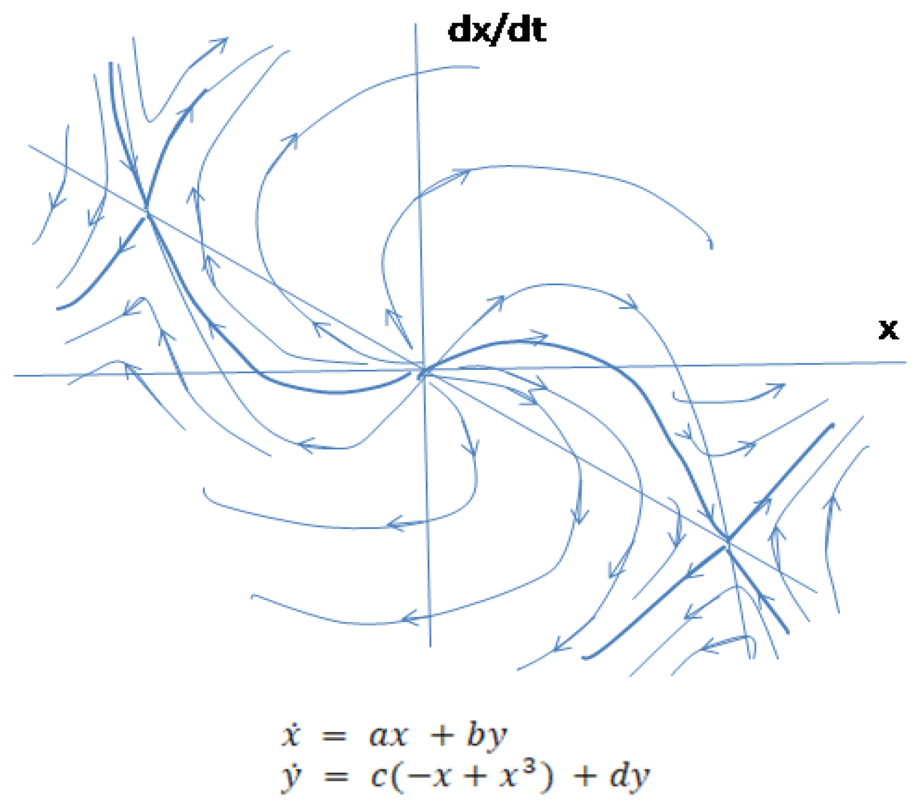
Figure 5.
Sketch of phase trajectories of a pendulum with small and large swings The system has two types of equilibrium points, elliptic and hyperbolic. Separatrices (red) form homoclinic trajectories (initial and end points are the same). Dark blue curves are small swings of the pendulum corresponding to low potential energy of the system. When the potential energy increases the trajectories of the large amplitude swings approach separatrices, which separate qualitatively different (elliptic from hyperbolic) types of trajectories. Blue trajectories correspond to the pendulum rotations.
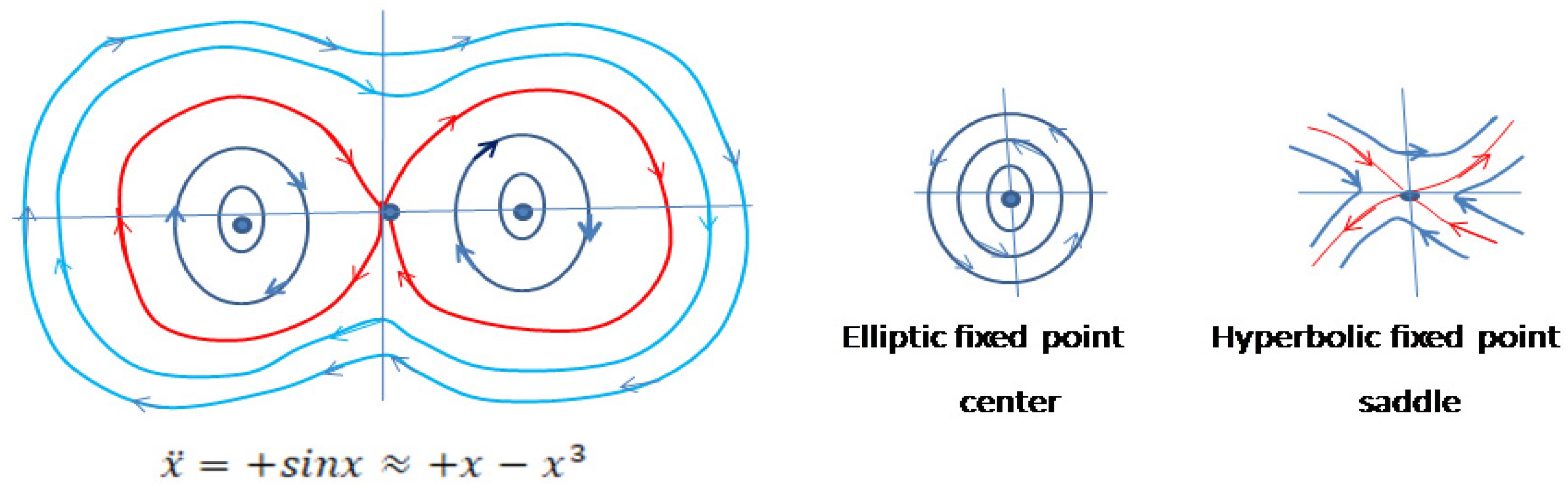
Figure 6.
Sketch of the phase portrait of the system with external forces in the plane around zero equilibrium point.
Figure 6.
Sketch of the phase portrait of the system with external forces in the plane around zero equilibrium point.
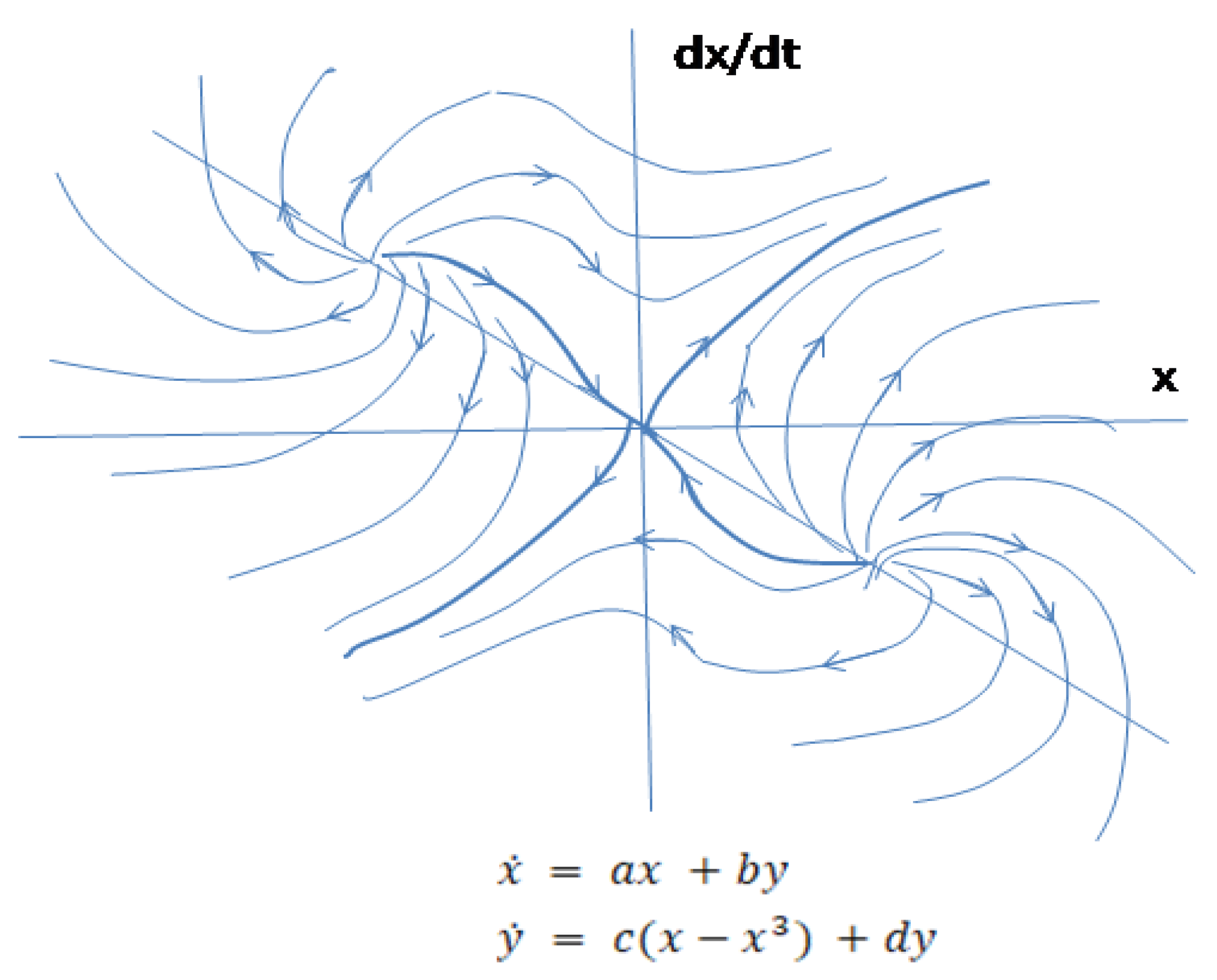
Figure 7.
Sketch of the divergent behavior of the system in polar coordinates Phase portrait of autonomous system with external forces. Diagonal elements (ax and cy) are added to the equation of the pendulum. Unstable foci corresponding to negative feedback are diverging towards saddle fixed point and coinciding with separatrices where the system bifurcates transforming unstable node to a saddle. The saddle corresponds to positive feedback. Positive feedback mechanism requires more energy than negative feedback.
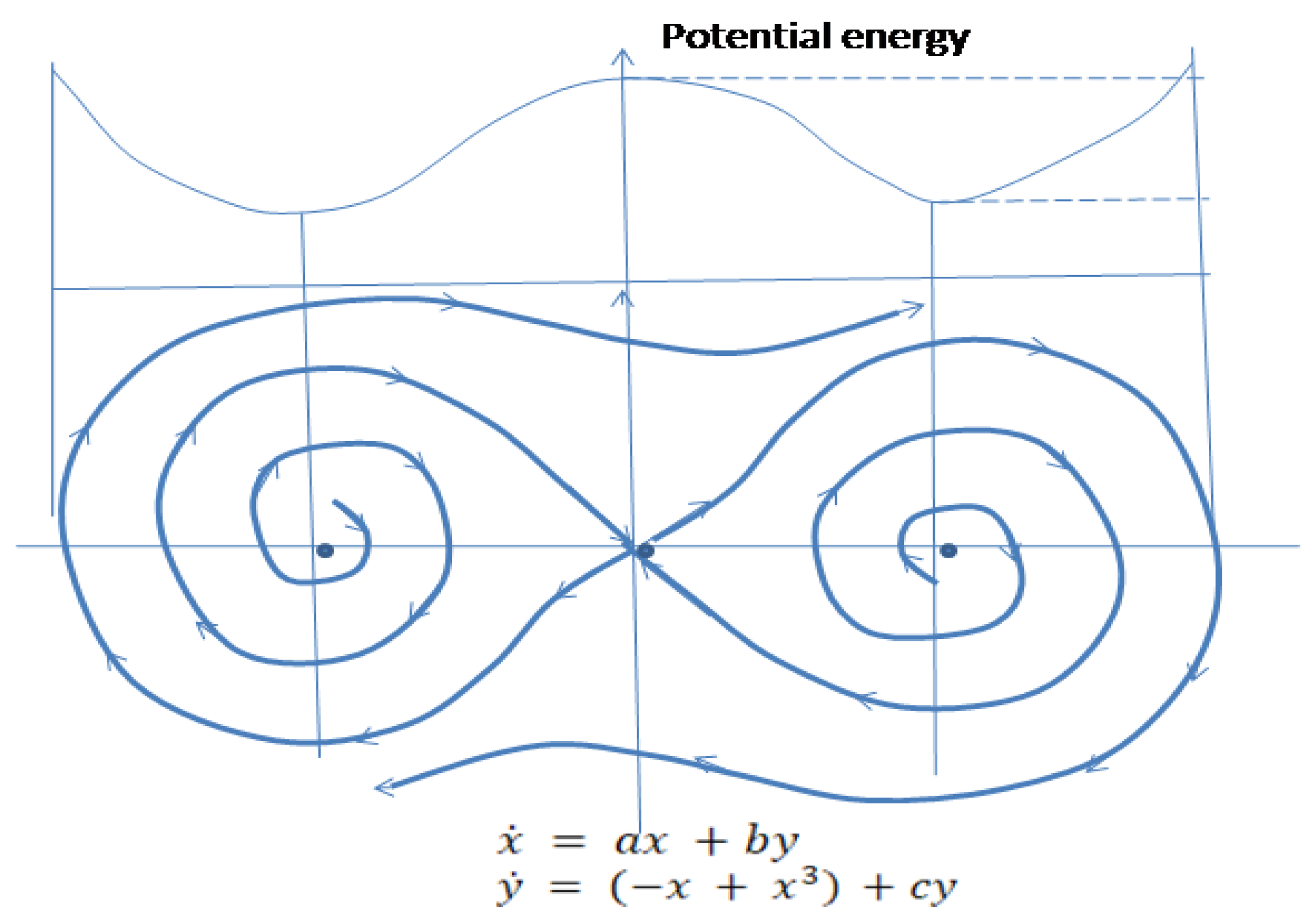
Figure 8.
Energy levels of conservative system not affected by environment a. Geometric image of coquaternion : hyperboloids of one sheet (blue); hyperboloids of two sheets(red); double cone (green). b. Equipotential surface(s) of hyperboloid(s) of one sheet transforms to a sphere and becomes closed, if total energy of the system maintains at the same level (conservative system without external forces). Outer closed trajectory indicates higher total energy level that possesses the system. Spiral trajectories sketch changes of the system’s conditions along geodesics. Arrows outside indicate the levels of critical points where hyperbolic hyperboloid transforms to a sphere and vice versa.
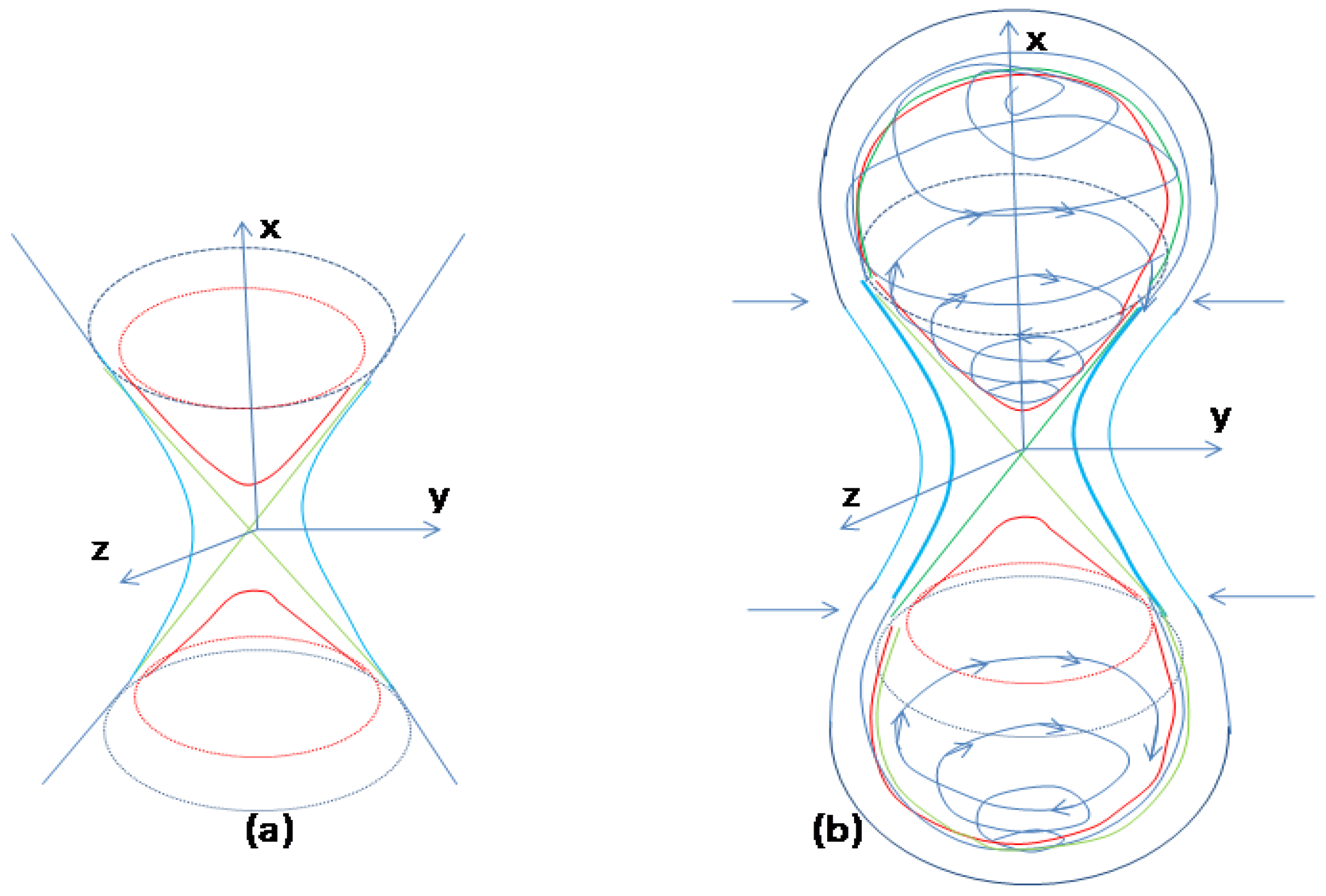
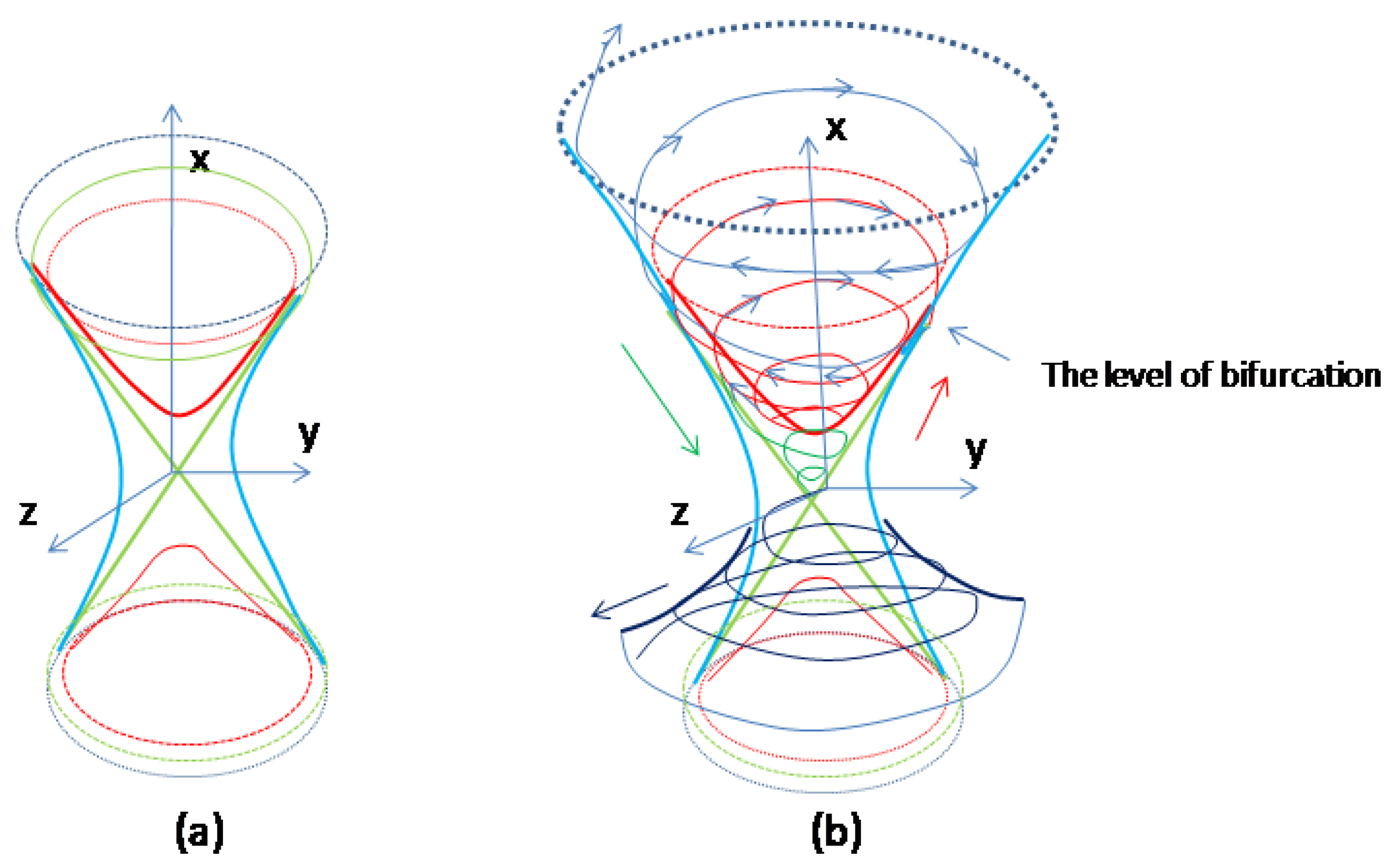
Figure 9.
Sketch of the systems dynamics affected by external forces. a. Coquaternion surfaces: hyperboloids of one sheet (blue); hyperboloids of two sheets (red); double cone (green). b. After negative feedback reaches a critical (bifurcation) point positive feedback is activated. At the critical point the parameterized curve changes the surface of elliptic hyperboloid (red) and continue travelling “downwards” along the upper cone (green) as a separatrix until reaches the equilibrium point. The corresponding curve on the plane will be the stable separatrix. Another curve of the stable separatrix comes from the opposite sheet of elliptic hyperboloid (not shown). Unstable separatrices trajectories diverge from equilibrium due to external environmental forces (black, demonstrated on the bottom).
Disclaimer/Publisher’s Note: The statements, opinions and data contained in all publications are solely those of the individual author(s) and contributor(s) and not of MDPI and/or the editor(s). MDPI and/or the editor(s) disclaim responsibility for any injury to people or property resulting from any ideas, methods, instructions or products referred to in the content. |
© 2024 by the authors. Licensee MDPI, Basel, Switzerland. This article is an open access article distributed under the terms and conditions of the Creative Commons Attribution (CC BY) license (http://creativecommons.org/licenses/by/4.0/).
Copyright: This open access article is published under a Creative Commons CC BY 4.0 license, which permit the free download, distribution, and reuse, provided that the author and preprint are cited in any reuse.


