Interactions Between Business Cycles, Financial Cycles and Monetary Policy in South Africa: A Unified Macroeconomic Framework

1. Introduction

Prior to the 2007-2009 Global Financial Crises (GFCs), Business Cycle (BC) studies were primarily based on Real Business Cycle (RBC) models and New Keynesian models (NKM) that disregarded financial factors (Kydland and Prescott, 1982; Long Jr and Plosser, 1983). The primary focus of these studies was on the dynamics of real indicators such as; consumption, rates of unemployment and employment, aggregate prices and gross domestic product (GDP), to name only a few. Important financial variables such as credit, house prices, equity and spreads were overlooked in such studies (Ma and Zhang, 2016). Yet, this did not mean that macroeconomists have discarded financial considerations in shaping their macroeconomic activity thoughts. A number of studies have been conducted with emphasis being solely on the interactions of the real economy and the financial system, explicitly, the incorporation of financial factors in BC models (Adrian and Liang, 2016; Ajello, Goldberg, and Perez-Orive, 2018; Fadeyi, Sedibe, van der Westhuizen, and Igene, 2019; Godwin, Howse, and Ramsey, 2017; Gurley and Shaw, 1955; Kindleberger and Kindleberber, 1978; Minsky, 1992).

Notwithstanding the enormous amount of work done on the importance of incorporating financial factors in BC models, the analysis of financial factors and financial shocks as sources of BC fluctuations has also received less attention prior to the 2007-2009 GFCs (Ma and Zhang, 2016). In reality, following the RBC literature (King and Rebelo, 1999), the conventional view about sources of BC fluctuations has been primarily centred on technological shocks, little or no role was found to be played by financial factors. This is especially the case in developed countries such as the United States, United Kingdom, and China, to name only a few (Ma and Zhang, 2016; Ajello, 2016; Ajello et al., 2018). In developing countries such as South Africa, the conventional view about sources of economic fluctuations has been centred on factors such as, the lack of resource endowment, low levels of human capital, the administrative, legal and institutional framework, the stance of the macroeconomic framework and structural policies (Ndlela and Nkala, 2003; Redl, 2018; Yıldız, Hesami, Rjoub, and Wong, 2021).

In the aftermath of the 2007-2009 GFCs, however, the view regarding sources of BC fluctuations expanded to include financial factors. For example, in Jermann and Quadrini (2012) a model with debt and equity financing was developed to explore the macroeconomic effects of financial shocks. Results revealed that financial shocks contributed significantly to observed dynamics of financial and real variables. This is in line with the conclusions of other related studies (Christensen and Dib, 2008; Hirakata, Sudo, and Ueda, 2011). From a general equilibrium model (DSGE) perspective, as estimated in Iacoviello (2015), it was found that financial shocks, that affect leveraged sectors, accounted for two-thirds of the output collapse during the great moderation. Recently, Caldara, Fuentes-Albero, Gilchrist, and Zakrajšek (2016) found that financial shocks have significant adverse effects on economic outcomes and were an important source of cyclical fluctuations since the 1980s. Similar conclusions are also found in recent contributions by Ajello, Laubach, Lopez-Salido, and Nakata (2016) and Ajello et al. (2018) among others.

So far, the enormous amount of theoretical as well as empirical studies, especially those in the aftermath of the 2007-2009 GFCs, has strongly argued about the linkages between the financial system and the real economy, specifically, the importance of FCs in BC models (Claessens, Kose, and Terrones, 2012; Ma and Zhang, 2016). To date, there exists near consensus among central bankers, economists and other scholars that FCs are an important source of BC fluctuations. While such issues are at the heart of the South African Reserve Bank (SARB)’s research agenda, according to authors’ knowledge, no study has adopted a composite index to measure a FC and its relationship with the BC and MP within a unified macroeconomic framework for South Africa, to address the above important avenue of research.

In this context, the present article aims to provide new empirical evidence on these unexplored avenues of research, within South Africa, through the exploration of the interactions between BCs, FCs, and MP within an extended New Keynesian model. Firstly, a Composite Financial Cycle index (CFCI) is constructed through the adoption of a Markov Switching Dynamic Factor Model. Secondly, it is asked, what is the role of the FC in BC fluctuations: is there a possible unified macroeconomic framework in South Africa? As a response, the article extends the traditional three equation New Keynesian model by incorporating the impact of the FC. Hence, through the adoption of a Multiple Equation Generalised Method of Moments (MEGMM), the article estimates a four equation New Keynesian model that features a link between the financial system and the South African real economy.

2. Conceptual framework

After the construction of a CFCI as an improved version of the South African FC, as a second step in this analysis, the article analyses the role of a FC in determining aggregate demand. To achieve this, the present article trails on the footsteps of Goodhart and Hofmann* (2005) and extend the traditional IS curve equation through incorporating the CFCI in the aggregate demand function. As a point of departure from the widely applied forward-looking IS curve, a backward-looking component of aggregate demand is also included in this model to capture habit formation and the associated adaptive manner in aggregate expenditure (Goodhart and Hofmann*, 2005; Ma and Zhang, 2016).

$$y_t=\mu E_t{y}_{t+1}+{\alpha }_1{y}_{t-1}+{\alpha }_2{y}_{t-2}+{\beta }_1\left(r_t-E_t{\pi }_{t+1}\right)+{\beta }_{2}C{FCI}_t+{\epsilon }_t^y$$

(1)

where $y_t$ is the output gap (Real GDP), $r_t-E_t{\pi }_{t+1}$ shows the real interest rate, ${CFCI}_t$ shows the composite financial cycle index and ${\epsilon }_t^y~iid. N(0, {\sigma }_y^2)$ is a demand shock. While the traditional NK IS curve relates the output gap to the expected future output gap and the ex-ante real interest rate only. The extended hybrid IS curve of this analysis differs from the conventional NK IS curve as it also captures the role played by the financial system on macroeconomic models (Goodhart and Hofmann*, 2005).

As a third step in this analysis, the article extends the traditional three equation New Keynesian model by incorporating the impact of a FC in the model system thus, making it a four equation New Keynesian Model. The traditional model reduces the economy to a three-equation system comprising, the traditional IS curve equation, the Philips curve and the conventional Tailor rule. The four-equation model of this analysis differ from the traditional three equation model since it features, an extended Hybrid IS curve, capturing the impact of the CFCI in aggregate demand. A Phillips curve which has both forward and backward-looking properties. Further, it is extended with a FC equation, capturing the cyclical fluctuation of the financial system, and the conventional Tailor rule capturing monetary policy behaviour, as follows.

The extended Hybrid IS curve.

The extended hybrid IS curve adopted in this analysis, is represented by equation 1 above.

The Phillips curve.

The Phillips curve considered in this analysis features both forward and backward-looking components of inflation in addition to the standard explanatory variable of the output gap. This is illustrated by the following equation:

$${\pi }_t={\beta }_1{E\pi }_{t+1}+\left(1-{\beta }_1\right){\pi }_{t-1}+{\beta }_2{y}_t+{\epsilon }_t^{\pi }$$

(2)

where the coefficient values of ${\beta }_1$ and $\left(1-{\beta }_1\right)$ are used to capture the extent of forward and backward-looking elements of inflation, respectively; $y_t$ is the output gap and ${\epsilon }_t^{\pi }$ $~iid. N(0, {\sigma }_{\pi }^2)$ is a supply shock. Such an incorporation of forward and backward-looking elements finds root in the theoretical model of staggered price setting as found in Scheibe and Vines (2005).

The Financial cycle.

The equation used to capture the evolution of the financial cycle as motivated by the stylized facts of the financial system given as follows:

$${FC}_t={\theta }_1{FC}_{t-1}+{\theta }_2{y}_t+{\theta }_3{r}_t+{\epsilon }_t^{FC}$$

(3)

where the coefficient ${\theta }_1$ captures the persistence nature of the financial cycle, ${\theta }_2$ capture the procyclical nature of the FC, ${\theta }_3$ captures the effect of MP on the FC and ${\epsilon }_t^{FC}$ $~iid. N(0, {\sigma }_{\pi }^2)$ is the FC shock. As the FC typically exhibits a considerable degree of persistence and co-movement with the BC, the coefficients ${\theta }_1$ and ${\theta }_2$ are expected to have positive signs. The sign on the coefficient ${\theta }_3$ is expected to be negative due to the fact that, an increase in the interest rate is associated with a FC downturn (Ma and Zhang, 2016).

The Monetary policy rule.

As prevalent in the literature, it is assumed that the central bank sets the nominal interest rate in accordance with a forward-looking conventional Tailor Rule. This includes interest rate smoothing and systematic responses to inflation and the output gap, given by the following equation:

$$r_t={\varnothing }_0+{\varnothing }_1{\pi }_{t+k}+{\varnothing }_2{y}_{t+p}+{\sum }_{i=1}^p{\rho }_i{r}_{t-i}+{\epsilon }_t^r$$

(4)

where ${\rho }_1$ is the interest rate smoothing parameter, ${\varnothing }_1$ and ${\varnothing }_2$ shows the preferences of the central bank with respect to inflation and output gap stabilization, ${\epsilon }_t^r~iid. N(0, {\sigma }_{\pi }^2)$ is an exogenous monetary policy shock (Ma and Zhang, 2016; Taylor and Williams, 2010; Verona, Martins, and Drumond, 2017).

3. Review of empirical literature

Conceptually, interactions between macroeconomics and financial indicators are mostly amplified in the presence of financial frictions. This mainly occurs through the financial accelerator and other related mechanisms operating through the firms, households and the countries’ balance sheets (Campbell, 2003). According to these mechanisms, an increase in asset prices leads to an improvement in the entity’s net worth, thus, enhancing its borrowing, investment and spending capabilities vis-à-vis. Such a process has the potential to lead to an amplified change in asset prices and having general equilibrium effects (Bernanke, Gertler, and Gilchrist, 1999; Gertler and Hubbard, 1988; Kiyotaki and Moore, 1997).

To date, some studies have focused on asset prices and credit as the main driving force of financial cycles (Adrian, Estrella, and Shin, 2010; Adrian and Shin, 2009). While other studies utilising models of frictions on open economies and emerging market economies, have considered how the dynamics of asset prices and exchange rates relates to the business cycle. For instance, Céspedes, Chang, and Velasco (2002) extended the standard financial accelerator mechanism and showed that adverse external shocks can have magnified impact on output due to balance sheet effects arising from currency devaluation. This avenue of research has also considered how gyrations in asset prices can affect the value of collateral required for international funding. In Mendoza (2010), it was shown that, when borrowing levels are high relative to asset value, shocks to collateral constraints can generate an amplified mechanism.

Empirically, it is known that, prior to the 2007-2009 GFC, a number of BC studies were mainly based on macroeconomic models that abstracted from the impact of financial factors on macroeconomic fluctuations (Kydland and Prescott, 1982; Long Jr and Plosser, 1983; King and Rebelo, 1999). According to these studies, the conventional view about sources of BC fluctuations has been centred on technological shocks, so much so that these were found to explain a considerable degree of variation in BCs (King and Rebelo, 1999). While such inference was mostly common in the general equilibrium literature, the structural VAR literature has pointed to other disturbances as the main sources of BC fluctuations and rarely found technological shocks to explain more than a quarter of output variations (Fisher, 2006; Galí, 2004).

In line with the structural VAR literature, developing country studies have pointed to other disturbances as the main source of BC fluctuations. For example, in Ndlela and Nkala (2003) an empirical analyses of macroeconomic fluctuations in South Africa was provided. The analyses showed that lack of resource endowment, low levels of human capital, the administrative, legal and institutional framework, the stance of the macroeconomic framework and structural policies were the main sources of BC fluctuations in South Africa. Further, it was concluded that, money supply and the world interest rate accounted for 30 percent and 18 percent of output fluctuations respectively, and the real exchange rate fluctuations were mostly associated with MP (Ndlela and Nkala, 2003). Therefore, the several number studies (Fisher, 2006; Galí, 2004) on BC fluctuations especially those prior to the 2007-2009 GFC, has pointed to other disturbances as sources of BC fluctuations, little or no evidence was provided on the role of financial factors in BC fluctuations.

However, the aftermath of the 2007-2009 GFC and the amount of costs imposed on the economies of different countries, led to an expansion in the view regarding sources of BC fluctuations to cater for the effect of financial factors. It has also led to an amplified interest in studying financial aspects of the BC (Hollander, 2017; Hollander and Van Lill, 2019; Justiniano, Primiceri, and Tambalotti, 2010; Ma and Zhang, 2016; Smets, 2014). For instance, Christiano, Motto, and Rostagno (2010) augmented a standard monetary DSGE model by including financial factors and fitted the model to the Euro Area and United States data. A new shock originating from the financial sector which accounted for a substantial portion of BC fluctuations, was found. Correspondingly, in Hafstead and Smith (2012) a standard BGG model was expanded through the introduction of bank production functions that implied a positive marginal cost for banks to originate loans and accept deposits. Results showed that, financial shocks both on the demand and supply sides, can cause severe macroeconomic fluctuations.

Further, a model with explicit roles for debt and equity financing was developed to explore how the observed dynamics of real and financial variables are affected by financial shocks. It was found that financial shocks contributed significantly to the observed dynamics of real and financial variables (Jermann and Quadrini, 2012). Furthermore, based on the supposition that BCs are financial rather than real, a DSGE model was estimated in Iacoviello (2015), where a recession was initiated by losses suffered by banks. Results showed that redistribution and other financial shocks that have effects on leveraged sectors accounted for two-thirds of the output collapse of the great depression. Similar findings are also found in other studies such as, Mandelman (2010) and Ajello (2016). These authors also considered shocks originating from the financial sector and proposed that such shocks could play a significant role as sources of BC fluctuations.

Recently, utilising a penalty approach within a Structural VAR framework, Caldara et al. (2016) found that financial shocks possesses significant adverse effects on macroeconomic outcomes, and such shocks were an important source of cyclical fluctuation since mid-1980s. Most recently, Ajello et al. (2018) developed a monetary DSGE model to study which financial shocks drive the BC. Estimating the model on US data, the authors found that sentiment shocks generated plausible BC responses and that they explained 20% of investment and employment fluctuations. In general, while an enormous amount of work has been conducted on this topic, this is mainly bias towards developed nations such as the US, the UK, China, to name only a few. In developing countries such as South Africa, this topic remains largely unexplored and literature is yet to discover its importance.

To date, an enormous amount of studies both empirical and theoretical has strongly argued about the interactions and linkages between BCs and FCs and the role of financial factors in shaping macroeconomic fluctuations (Ajello et al., 2018). This has led to increasing consensus among economists, central bankers and other scholars that, the financial system plays a significant role as a source of macroeconomic fluctuations, therefore, the FC is an important source of BC fluctuations, see (Ajello, 2016; Ajello et al., 2018; Caldara et al., 2016; Christensen and Dib, 2008; Christiano and Ikeda, 2013; Christiano et al., 2010; Hafstead and Smith, 2012; Hirakata et al., 2011; Iacoviello, 2015; Ma and Zhang, 2016).

In South Africa, like any other central bank around the globe, there is currently, a clear mandate for financial stability within the SARB. In accordance with the Financial Sector Regulations Bill (FSR Bill), it is the SARB’s responsibility to protect and enhance financial stability in South Africa. If a systemic event is identified as imminent or has occurred, it is also the SARB’s responsibility to maintain or restore stability (Bank, 2016). Therefore, the SARB must take all necessary steps to thwart systemic events from stirring and to alleviate the hostile effects of events on financial stability through the application of toolkits of MaPP instruments.

While the topics of the interactions of the real economy and the financial system and many others currently form part of the SARB’s research agenda. According to authors’ knowledge, no study has attempted to develop a unified macroeconomic framework for policy analyses in South Africa, despite several calls for such a framework. Further, no study has adopted a composite index to improve the current South African FC and to analyse its relationship with the BC and MP within a unified macroeconomic framework for South Africa. As a result, the present article contributes to the literature through developing a unified macroeconomic policy framework for South Africa, featuring a link between the real economy and the financial system. The article further contributes to the literature through the improvement of the current South African FC and the measurement of its relationship with the BC and MP within a unified macroeconomic framework setting.

4. Methodology

4.1. Data Source and Variables Description

An extensive database was constructed using monthly time series of financial and economic variables for South Africa, penning the period 2000M01 to 2018M12. This period is informed by the availability of FC data and the desire to focus on the periods before, during and after the 2007 -2009 GFCs. While literature has not yet reached consensus on the time series indicators that should be utilised to measure FCs, this article trails on the footsteps of Krznar and Matheson (2017), Chorafas (2015), Ma and Zhang (2016), among others, to measure the CFCI. Accordingly, this article adopted thirteen (13) monthly financial time series variables to measure the CFCI. The specific CFCI variables, descriptions and data sources are shown in Tables 1.

Other important variables utilised includes, Real Gross Domestic Product (RGDP), which represents a monthly measurement of economic output taking into consideration the effect of inflation. Short-term interest rates (STIR): which are rates showing how short-term borrowings are affected between financial institutions. Inflation (INF): proxied by CPI inflation, is defined as the change in the price of a basket of goods and services that are purchased by specific groups of households. Expected inflation (EINF): representing the survey-based inflation forecasts. And Long-term interest rates (LTIR): which refers to Government bonds maturing in ten years.

As an initial step towards the construction of the CFCI, all data series were seasonally adjusted and for preparation purposes, the article followed on the footsteps of Ma and Zhang (2016) and converted all the variables to a single unit of measure. This was achieved through the adoption of a min-max normalisation technique given as follows:

$$V_{it}^{’}={\displaystyle \frac{V_{it}-Min\left(V_i\right)}{Max\left(V_i\right)-Min\left(V_i\right)}}$$

(5)

where $V_{it}$ is the value of variable $i$ during period $t$; $Min\left(V_i\right)$ and $Max\left(V_i\right)$ denotes minimum and maximum values of the sample period, respectively. This is shown by variable $i$ in the sample period $t$. $V_{it}^{’}$, on the other hand, shows the normalized value of the variables. Once all the variables are in a single unit of measure, the methodology discussed below is adopted to measure the CFCI.

4.2. Composite Financial Cycle Index Development Approach

This article proposes a two-step Markov Switching Dynamic Factor Model in state space form, which was first proposed by Kim (1994), as a suitable model to study the South African financial cycle. The analysis trails on the same kind of specification as in Kim and Yoo (1995) and assume that the growth rate cycle has two states, viz: downturn and upturn. Financial sector activity in this case is represented by an unobservable factor extracted from an amalgamation of several observable variables.

The model is divided into two equations: the first equation defines a factor model, and the second equation defines a Markov Switching Dynamic Regression Model, which is assumed for the common factor. Precisely, the first equation shows each series of the information set decomposed into the sum of a common component and an idiosyncratic component as follows:

$$y_t={\gamma f}_t+z_t$$

(6)

where $y_t$ is an $N\times 1$ vector of economic indicators, $f_t$ is a univariate common factor, $z_t$ is an $N\times 1$ vector of idiosyncratic components, which is uncorrelated with $f_t$ at all leads and lags, $\gamma$ is an $N\times 1$ vector. The requirement from this equation is for all variables to be stationary, i.e. all individual indicators are detrended and only the cyclical components of these indicators are adopted for the analysis at hand (Doz and Petronevich, 2016).

The second equation defines a Markov Switching model of Hamilton (1989). This model has the ability to mark time. In terms of this model, a latent random variable $s_t$ governs the state or regime with $s_t=0$ indicating low or negative growth, and $s_t^{*}=1$ indicating high or positive growth. Two states signifying positive and negative average growth rates are adequate to mark turning points since $∆y_t<0$ indicates a downturn and $∆y_t>0$ indicates an upturn (Bosch and Ruch, 2013).

Markov-switching regression models allow the parameters to vary over the unobserved states. In the simplest case, this model can be expressed as a Markov Switching Dynamic Regression model (MSDR) with a state-dependent intercept term as follows:

$$y_t={\mu }_{s_t}+{\epsilon }_t$$

(7)

Where ${\mu }_{s_t}$ is the parameter of interest, ${\mu }_{s_t}={\mu }_1$ when $s_t=1$, and ${\mu }_{s_t}={\mu }_2$when $s_t=2$. MSDR models allow a quick adjustment after the process changes state. These models are often used to model monthly to higher-frequency data. The MS-DFM model can be estimated in either one or two steps (Doz and Petronevich, 2016). The main limitation of the one-step estimation procedure is that it can only be estimated using a smaller set of variables. This approach is found too constrained for the purpose of this analysis. As a result, this article resorted to using a two-step estimation approach and proceeded as follows:

The first step involves the extraction of a common factor $f_t$ from an amalgamation of a large set of financial variables, according to equation 2 above, without the consideration of its Markov Switching dynamics. To this end, this article utilises both a Dynamic Factor Model and a Principal Component Analysis (PCA) method and considers that the first factor or principal component ${\widehat{f}}_t$ provides a good approximation of the common factor. In this context, the article estimated the following equation (9) to develop a CFCI for South Africa:

$$\left({\displaystyle \genfrac{}{}{0pt}{}{f_t}{f_{t-1}}}\right)=\left(\begin{array}{cc}{\theta }_1& {\theta }_2\\ 1& 0\end{array}\right)\left({\displaystyle \genfrac{}{}{0pt}{}{f_{t-1}}{f_{t-2}}}\right)+\left({\displaystyle \genfrac{}{}{0pt}{}{V_t}{0}}\right)$$

(8)

$$\left(\begin{array}{c}{∆RBEER}_t\\ {∆HP}_t\\ {∆ASP}_t\\ {∆GB10Y}_t\\ ∆{GB5Y}_t\\ {∆TCPFS}_t\\ {∆LTGBY}_t\\ {∆NEER}_t\\ {∆M1}_t\\ ∆{M2}_t\\ ∆{M3}_t\\ {∆TBILL}_t\\ ∆{ILR}_t\\ \end{array}\right)=\left({\displaystyle \genfrac{}{}{0pt}{}{\begin{array}{c}{\gamma }_1\\ {\gamma }_2\\ {\gamma }_3\\ {\gamma }_4\end{array}}{\begin{array}{c}{\gamma }_5\\ {\gamma }_6\\ {\gamma }_7\\ {\gamma }_8\\ {\gamma }_9\\ {\gamma }_{10}\\ {\gamma }_{11}\\ {\gamma }_{12}\\ {\gamma }_{13}\end{array}}}\right)f_t+\left({\displaystyle \genfrac{}{}{0pt}{}{\begin{array}{c}{\epsilon }_{1t}\\ {\epsilon }_{2t}\\ {\epsilon }_{3t}\\ {\epsilon }_{4t}\end{array}}{\begin{array}{c}{\epsilon }_{5t}\\ {\epsilon }_{6t}\\ {\epsilon }_{7t}\\ {\epsilon }_{8t}\\ {\epsilon }_{9t}\\ {\epsilon }_{10t}\\ {\epsilon }_{11t}\\ {\epsilon }_{12t}\\ {\epsilon }_{13t}\end{array}}}\right)$$

(9)

The second step estimates by Maximum Likelihood, the parameters of a MSDR. This was aimed at fitting a univariate model (as seen in Hamilton, 1989) to the estimated factor ${\widehat{f}}_t$ which is taken as if it were an observed variable. In order to identify the CFCI peaks and troughs, the article followed on the footsteps of Krznar (2011) and identified a peak of the CFCI in period t, if financial sector activity was on an upturn in period t-1 and filtered probability$Pr(s_{t+1}=1|{\Omega }_{t-1},p,q,{\mu }_1,{\mu }_2{\sigma }^2)\ge 0.5$, and a trough is defined in period t if financial sector activity was on a downturn in period t-1, and filtered probability$Pr(s_{t+1}=1|{\Omega }_{t-1},p,q,{\mu }_1,{\mu }_2{\sigma }^2)\le 0.5$.

4.3. Model specification for the interactions of FCs, BCs and MP

4.3.1. Generalised Method of Moments

As an initial step towards the analysis of the interactions between FCs, BCs and MP, the article examines the role of FCs in BC models, specifically analysing whether the FC represented by the CFCI plays an important role in determining aggregate demand. To archive this, the article trails on the footsteps of Goodhart and Hofmann* (2005), and extends the traditional IS-Curve equation through the incorporation of the CFCI variable in the aggregate demand function as in equation one above. To attain robust results, a Generalized Method of Moments (GMM) is utilised in the regression analysis.

GMM remains predominant in literature compared to the traditional estimation methods such as OLS, 2SLS and GLS. Compared with the traditional estimation methods abovementioned, the GMM method does not require complete knowledge of the underlying data distribution. It also controls for the endogeneity in explanatory variables, which is helpful in terms of avoiding the problem of biasedness due to model misspecification (Ma and Zhang, 2016). The traditional Method of Moments (MOM) acts as an initial step towards the estimation of GMM. This is based on the idea of estimating a population moment with the use of corresponding sample moment (Mittelhammer, Judge, and Schoenberg, 2005). The vector of$L$ moments to be satisfied by the true parameter $\beta$ can be written as:

$$E\left[m\right(y_{t },\beta \left)\right]=0$$

(10)

where $y_{t }$ is a vector of variables observed at time $t$ and $\beta$ is a unique value of a set of parameters that makes the expectation equal to zero. The above equation should always satisfy orthogonality conditions between a set of instrumental variables $Z_t$ and the residuals of the equation, $u_t\left(\beta \right)=u(y_t, X_t, \beta )$ as follows:

$$E\left[Z_t{\mu }_t\left(\beta \right)\right]=0$$

(11)

where $X_t$ shows the exogenous variables observable at time$t$. Through the replacement of the moment conditions in $E\left[m\right(y_{t },\beta \left)\right]=0$ by its sample analogue, we derive the following traditional Method of Moments estimator:

$$m_T={\displaystyle \frac{1}{T}}{\sum }_{t=1}^T{Z}_t{u}_t\left(\beta \right)={\displaystyle \frac{1}{T}}{Z}^{’}{u}_t\left(\beta \right)=0$$

(12)

where $T$ stands for the sample size. It is noted that the MOM can only have an exact solution to this equation if, and only if, the number of moment conditions denoted by $L$ is the same as the number of parameters denoted by$K$. However, this is normally not the case in many situations. In general, there are more moment conditions than the number of unknown parameters, thus$L > K$. This situation is referred to as over identification. It is under such conditions that the use of the traditional Method of Moments is found irrelevant and may lead to biased estimates. As a result, an alternative approach, namely Generalized Method of Moments, is adopted as it is able to deal with the so-called over identified system (Hall, 2005).

In a GMM method, one demarcates the magnitude by means of a generalized metric which is based on a positive semi-definite quadratic form. Suppose that $A$ is a metric for this quadratic form, then this metric is given by:

$${‖E_N\left[Z\epsilon \right]‖}_A={‖{\displaystyle \frac{1}{N}}{Z}^{’}\widehat{E}‖}_A\equiv N{\left({\displaystyle \frac{1}{N}}{Z}^{’}\widehat{E}\right)}^{’}A\left({\displaystyle \frac{1}{N}}{Z}^{’}\widehat{E}\right)={\displaystyle \frac{1}{N}}{\widehat{E}}^{’}ZA{Z}^{’}\widehat{E}$$

(13)

To derive a GMM estimate which is, in this case, going to be referred to as${\widehat{\beta }}_A^{’}$, one first minimizes the problem ${\widehat{\beta }}_A^{’}={argmin}_{\widehat{\beta }}{‖Z^{’}\widehat{E}‖}_A$ whose solution will be determined by$0={\displaystyle \frac{d}{d\widehat{\beta }}}{‖Z^{’}\widehat{E}‖}_A$. Applying the chain rule to expand this derivative, one gets:

$$0={{\displaystyle \frac{d}{d\widehat{\beta }}}‖Z^{’}\widehat{E}‖}_A={\displaystyle \frac{d}{d\widehat{E}}}{‖Z^{’}\widehat{E}‖}_A{\displaystyle \frac{d\widehat{E}}{d\widehat{\beta }}}={\displaystyle \frac{d}{d\widehat{E}}}\left({\displaystyle \frac{1}{N}}{\widehat{E}}^{’}\left(ZA{Z}^{’}\right)\widehat{E}\right){\displaystyle \frac{d(Y-X\widehat{\beta })}{d\widehat{\beta }}}={\displaystyle \frac{2}{N}}{\widehat{E}}^{’}ZA{Z}^{’}(-X)$$

(14)

As can be seen in the last step, the matrix identities ${\displaystyle \frac{dAb}{db}}=A$ and ${\displaystyle \frac{d\left(b^{’}Ab\right)}{db}}=2b^{’}A$ have been used, where $b$ represents a column vector and $A$ represents a symmetric matrix. Dropping the factors of ${\displaystyle \frac{-2}{N}}$ and transposing, the result is as follows:

$$0={\widehat{E}}^{’}ZA{Z}^{’}X={\left(Y-X{\widehat{\beta }}_A\right)}^{’}ZA{Z}^{’}X=Y^{’}ZA{Z}^{’}X-{\widehat{\beta }}_A^{’}{X}^{’}ZA{Z}^{’}X$$

(15)

$$\Rightarrow X^{’}ZA{Z}^{’}X{\widehat{\beta }}_A^{’}=X^{’}ZA{Z}^{’}Y$$

(16)

$$\Rightarrow \widehat{\beta }={\left(X^{’}ZA{Z}^{’}X\right)}^{-1}{X}^{’}ZA{Z}^{’}Y$$

(17)

This is a GMM estimator inferred by $A$ which is linear in$Y$. The GMM estimator is said to be consistent, which basically means that it converges in probability to $\beta$ as the sample size increases to infinity (Hansen, 1982). However, it is not unbiased, as discussed above. This is mainly because, in finite samples, the instruments are perfectly uncorrelated with the endogenous constituents of the instrumented regressors.

The above discussed GMM method is used to estimate the reduced form of the Hybrid IS curve, which features a link between the FC and the BC. It imposes the following orthogonality condition:

$$E_t\left\{{rGDP}_t-\left[\mu {rGDP}_{t+1}+{\alpha }_1{rGDP}_{t-1}+{\beta }_1{rr}_t+{\beta }_{2}C{FCI}_t\right]|v_t\right\}=0$$

(18)

where ${rr}_t=\left(r_t-E_t{\pi }_{t+1}\right)$ denotes the real interest rate as described above; $v_t$ is a vector of instrument variables at time period $t$ and it is orthogonal to ${\epsilon }_t$. The list of chosen instruments encompasses the lagged values of all endogenous variables and other exogenous variables able to predict inflation and the output gap. These instruments are uncorrelated with the disturbance terms and correlated with the explanatory variables. The following sub-section provides a discussion on the Multiple Equation GMM method.

4.3.2. A Multiple Equation Generalised Method of Moments technique

As a second step towards the analysis of the interactions between FCs, BCs, and MP, the article adopts a Multiple Equation Generalised Method of Moments (MEGMM) for the regression analysis of the four equation New Keynesian model as outlined in section two above. This method enables authors to handle a system of multiple equations, by suitably specifying the matrices and the vectors comprising a Single Equation Generalised Method of Moments (SEGMM). This multiple equation model can be expressed as a single equation GMM estimator (Hansen, 2010). In the presence of heteroscedasticity, the multiple equation GMM reduces to a Full-information Instrumental Variable Efficient (FIVE) estimator model. It further, reduces to a 3 Stage Least Squares model, where the set of instrumental variables is common through all the equations (Hall, 2005; Hansen, 1982, 2010).

With the assumption that all the regressors are predetermined, the 3SLS reduces to what is called Seemingly Unrelated Regressors (SUR), which in turn gives what is called Multivariate Regression (MR) when all the equations have the same regressors. A MEGMM can be represented as a system of equations with its coefficients constrained to be the same across equations. A GMM estimator with all the regressors predetermined and errors conditionally homoscedasticity, in this case is the random effect estimator. Thus, the SUR and MR are equivalent estimators (Hansen, 2010).

Several assumptions are made to derive a MEGMM estimator. These include the assumption of linearity: assume there are $M$ equations such that:

$$y_{im}=z_{im}^{’}{\delta }_m+{\epsilon }_{im} (m=\mathrm{1,2},\dots .,M;i=\mathrm{1,2},\dots \dots .,n)$$

(19)

where:

• $n =$ Sample size
• $z_{im }^{’} = L_m-$ Dimensional vector of regressors
• ${\delta }_m =$ The conformable coefficient vector and
• ${\epsilon }_{im} =$An unobservable error term in the $m$-th equation

The matrix representation of the linear multiple equation regression model can be represented by:

$$y=Z\delta + \epsilon$$

(20)

Where:

$$L={\sum }_{m=1}^M{L}_M$$

(21)

The second assumption is that of Ergodic stationarity: let $w_i$ be a unique and non-constant element of$(y_{i1},\dots ,y_{iM}, z_{i1},\dots ,z_{iM},x_{i1},\dots ,x_{iM})$, then, ${[w}_i]$ is jointly stationary and ergodic.

The third assumption is that of orthogonality conditions, which stipulates that, for each equation $m$, the $K_m$ variables in the instruments $x_{im}$ are predetermined such that:

$$E\left(x_{im}.{\epsilon }_{im}\right)=0 (m=\mathrm{1,2},\dots ,M)$$

(22)

There are in total ${\sum }_m{K}_m$ orthogonality conditions which in turn define:

$$\begin{array}{c}{g}_i\\ \left({\sum }_{m=1}^M{K}_{mx1}\right)\end{array}\equiv \left[\begin{array}{cc}{X}_{i1}& {\epsilon }_{i1}\\ X_{iM}& {\epsilon }_{iM}\end{array}\right]$$

(23)

The orthogonality conditions can be written compactly as$E\left(g_i\right)=0$. Note: this is not assuming cross-equation orthogonalities. Given the above orthogonality conditions, identification can be established in the same way as in the case of single equation GMM:

$$g\left(w_i;\delta \right)\equiv \left[\begin{array}{ccc}{X}_{i1}& \cdots & (y_{i1}-Z_{i1}^{’}{\delta }_1)\\ ⋮& \ddots & ⋮\\ X_{iM}& \dots & (y_{iM}-Z_{iM}^{’}{\delta }_M)\end{array}\right]$$

(24)

The orthogonality conditions can be expressed as$E\left[g\left(w_i;\tilde{\delta }\right)\right]=0$. The coefficient vector is identified if $\tilde{\delta }=\delta$ is the only solution to the system of the equations:

$$E\left[g\left(w_i;\tilde{\delta }\right)\right]=0$$

(25)

The moment conditions for each of the equations in the MEGMM are the same as the ones derived for the SEGMM model. In that sense, a system of equations determining $\tilde{\delta }$ can also be derived in the same way as:

$${\sum }_{xz}\tilde{\delta }={\sigma }_{xy}$$

(26)

The MEGMM ${\sum }_{xz}$ is block diagonal. Recall that a necessary and sufficient condition for identification of the SEGMM is that ${\sum }_{xz}$ be of full column rank. If $K_m$=$L_M$ for$(m=\mathrm{1,2},\dots ,M)$, then $\delta$ is exactly identified and

$$\left[\begin{array}{c}{\delta }_1\\ ⋮\\ {\delta }_M\end{array}\right]=\left[\begin{array}{c}{\sum }_{x_1{z}_1}^{-1}{\sigma }_{x_1{y}_1}\\ ⋮\\ {\sum }_{x_M{z}_M}^{-1}{\sigma }_{x_M{z}_M}\end{array}\right]$$

(27)

If $K_m>L_M$ for some$m$, then solving

$$E\left[g_i\left(\delta \right)\right]=\begin{array}{c}{\sigma }_{xy}\\ \left(kx1\right)\end{array}-\begin{array}{c}{\sum }_{xz}\\ \left(KxL\right)\end{array}\begin{array}{c}\tilde{\delta }\\ \left(Lx1\right)\end{array}$$

(28)

requires the rank condition which posit that: for each $m\left(=\mathrm{1,2},\dots ,M\right), E\left(x_{im}{z}_{im}^{’}\right)\left(K_{m}x{L}_m\right)$ is of full rank. This means that all coefficient vectors (${\delta }_1,\dots \dots .,{\delta }_M$) can be determined uniquely if and only if each coefficient vector ${\delta }_M$ is uniquely determined. This is the case if the orthogonality assumption holds for each equation.

The last of these assumptions is that $g_i$ is a martingale difference sequence with finite second moments i.e. [$g_i$] is a joint martingale difference sequence. $E\left(g_i{g}_i^{’}\right)$ is non-singular.

If $K_m=L_M$ for $m=1,\dots .,M$ then $X_m^{’}{Z}_m$ is a square matrix and so:

$${\tilde{\delta }}_m=S_{x_m{z}_m}^{-1}{S}_{x_m{y}_m}, m=1,\dots \dots .,M$$

(29)

Therefore:

$$\tilde{\delta }={({\tilde{\delta }}_1,\dots \dots .,{\tilde{\delta }}_M)}^{’}$$

(30)

Solves:

$$\begin{array}{c}{S}_{xy}\\ \left(kx1\right)\end{array}-\begin{array}{c}{S}_{xz}\\ \left(KxL\right)\end{array}\begin{array}{c}\tilde{\delta }\\ \left(Lx1\right)\end{array}=0$$

(31)

If the equation is identified and $K_m>L_{M }$for some$m$, then it is impossible to discover $\tilde{\delta }$ that solves the moment conditions. Thus, for the overidentified model, we let $\widehat{W}$ be a $K\times K$ positive definite symmetric matrix given below as:

$$\widehat{W}=\left[\begin{array}{cc}{\widehat{W}}_{11}& {\widehat{W}}_{12}\\ {\widehat{W}}_{12}^{’}& {\widehat{W}}_{22}\\ \begin{array}{c}⋮\\ {\widehat{W}}_{1M}^{’}\end{array}& \begin{array}{c}⋮\\ {\widehat{W}}_{2M}^{’}\end{array}\end{array} \begin{array}{cc}\cdots & {\widehat{W}}_{1M}\\ \cdots & {\widehat{W}}_{2M}\\ \begin{array}{c}\ddots \\ \cdots \end{array}& \begin{array}{c}⋮\\ {\widehat{W}}_{MM}\end{array}\end{array}\right]$$

(32)

such that $\begin{array}{c}\widehat{W}⟶W\\ p\end{array}$. The GMM estimator then solves:

$$\tilde{\delta }\left(\widehat{W}\right)\begin{array}{c}argmin J\left(\tilde{\delta }, \widehat{W}\right)\\ \tilde{\delta }\end{array}=n{g}_n{\left(\tilde{\delta }\right)}^{’}\widehat{W}{g}_n\left(\tilde{\delta }\right)$$

(33)

$$=\begin{array}{c}argmin \\ \tilde{\delta }\end{array}n{\left(S_{xy}-S_{xz}\tilde{\delta }\right)}^{’}\widehat{W}(S_{xy}-S_{xz}\tilde{\delta })$$

(34)

The definition of the MEGMM estimator is the same as in the case of a SEGMM, given that the weighing matrix$\widehat{W}$ is now${\sum }_m{K}_{m}x{\sum }_m{K}_m$. Thus, given the above features and assumptions, the multiple equation GMM estimator is given by:

$$\tilde{\delta }\left(\widehat{W}\right)={\left(S_{xz}^{’}\widehat{W}{S}_{xz}\right)}^{-1}{S}_{xz}^{’}\widehat{W}{S}_{xy}$$

(35)

and its sampling error is given by:

$$\tilde{\delta }\left(\widehat{W}\right)-\delta ={\left(S_{xz}^{’}\widehat{W}{S}_{xz}\right)}^{-1}{S}_{xz}^{’}\widehat{W}\overline{g}$$

(36)

$$S_{xz}^{’}\widehat{W}\overline{g}$$

(37)

where:

• $S_{xy}=$Is a stacked vector,
• $S_{xz}=$ Is a block diagonal matrix,
• ${\sum }_m{K}_{m}x{\sum }_m{K}_m=$ Is the size of the weighting matrix
• $\overline{g}=$ Is the sample mean of${ g}_i$, is the stacked vector given by:

$$\overline{g}\equiv {\displaystyle \frac{1}{n}}{\sum }_{i=1}^n{g}_i=\left[\begin{array}{cc}\begin{array}{c}{\displaystyle \frac{1}{n}}{\sum }_{i=1}^n{x}_{i1}\\ {\displaystyle \frac{1}{n}}{\sum }_{i=1}^n{x}_{iM}\end{array}& \begin{array}{cc}\begin{array}{c}\begin{array}{c}\cdots \\ ⋮\end{array}\\ \cdots \end{array}& \begin{array}{c}\begin{array}{c}{\epsilon }_{i1}\\ ⋮\end{array}\\ {\epsilon }_{i1}\end{array}\end{array}\end{array}\right]=g_n\delta$$

(38)

Given all the features as abovementioned, it would be necessary to write out the MEGMM estimator as shown in equation 18, in full. To achieve this, it would be required that ${\widehat{W}}_{mh}(K_m\times K_h)$ be the $(m,h)$ block of $\widehat{W}(m,h=\mathrm{1,2},\dots ,M)$.

The present article utilises this method in order to get unbiased estimates of the four equation New Keynesian model. Accordingly, assume that $v_1$, $v_2$, $v_3$, and $v_4$ denotes the instruments for all the four equations in the model, respectively. The set of moment conditions can be illustrated mathematically as follow:

$$E_t\left\{\begin{array}{c}{rGDP}_t-\left[{\alpha }_0+\mu {rGDP}_{t+1}+{\alpha }_1{rGDP}_{t-1}+{\beta }_1{rr}_t+{\beta }_{2}C{FCI}_t\right]|v_1\\ {INF}_t-\left[{{\gamma }_0+\gamma }_1{INF}_{t+1}+\left(1-{\gamma }_1\right){INF}_{t-1}+{\gamma }_2{rGDP}_t\right]|v_2\\ {CFCI}_t-{[{[\theta }_0+\theta }_1{CFCI}_{t-1}+{\theta }_2{rGDP}_t+{\theta }_3{r}_t\left]\right|v_3\\ {INT}_t-[{\varnothing }_0+{\varnothing }_1{INF}_{t+k}+{\varnothing }_2{rGDP}_{t+p}]|v_4\end{array}\right\}=0$$

(39)

The chosen instruments are orthogonal to the error terms and are different for each equation. The list of chosen instruments per equation encompasses the lagged values of all endogenous variables and other exogenous variables able to predict inflation and the output gap. These instruments are uncorrelated with the disturbance terms and correlated with the explanatory variables per equation.

To test for the validity of these GMM methods, the present article conducts various tests which include the instruments orthogonality test also referred to as the C-test, the regressor endogeneity test which is carried out through the application of the Durbin-Wu-Hausman test, and lastly, the weak instrument diagnostic test which is carried out through moment selection criteria. These are all discussed in the appendix of this article.

5. Estimation results and analysis

5.1. Results on the Measurement of the Composite Index

The initial step of this analysis involved the measurement of the Composite Financial Cycle Index. This was achieved through the adoption of a two-step Markov Switching Dynamic Factor Model in State-Space form (DFM-SSF). Results from this are shown below.

First Step: DFM

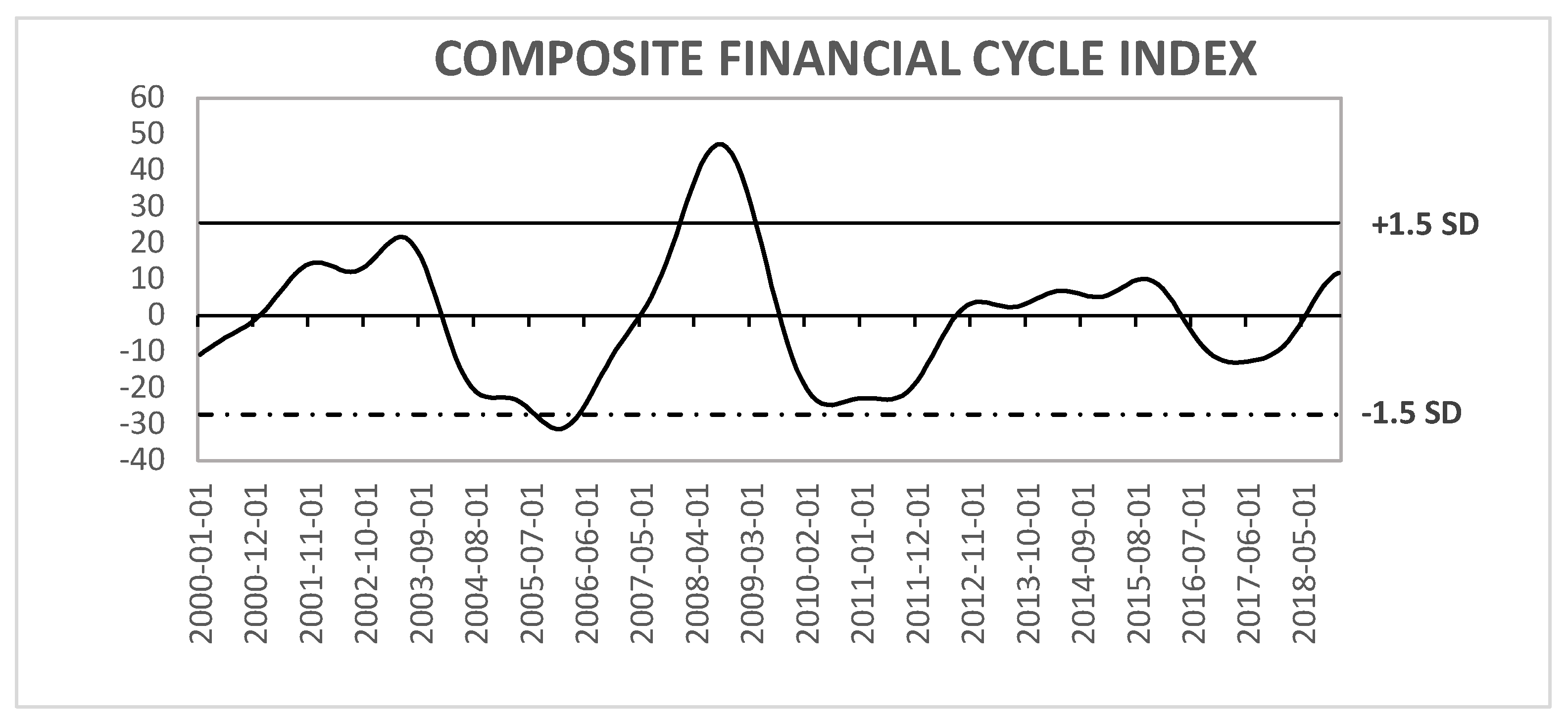
In the first step of this procedure, a common factor was extracted from an amalgamation of eleven financial time series variables. Applying a DFM-SSF and Principal Component Analysis (PCA), it was considered that the first factor and the first principal component provides a good approximation of the common factor. This common factor is here referred to as the composite financial cycle index (CFCI), and is illustrated in Figure 1.

Figure 1 shows the CFCI relative to the ±1.5 standard deviation boundaries. The CFCI captures with accuracy both the periods of instabilities and imbalances. The main events such as the 2001 Rand crises and the 2007-2009 GFC seem to be captured well by the index. Further, the index indicates that both upwards (potential build-up of imbalances) and downwards (manifestation of instabilities) phases, are meaningful signals about financial instabilities.

Figure 1. DFM-SSF Financial Cycle Index. Source: Authors’ own estimates

Figure 1. DFM-SSF Financial Cycle Index. Source: Authors’ own estimates

Second step: Markov Switching Dynamic Regression Model

Table 2 shows the results of the turning points of the CFCI, as obtained from the filtered probabilities of the MSDR model. Based on the rule (see section 4.2) for turning points identification in view of filtered probabilities. We identified two peaks of the CFCI: one in May 2003 and another in September 2008 (see Table 2). These are the highest points that marks the end of expansion and the beginning of contraction periods in financial activity.

We further identified two troughs of the CFCI: one in January 2006, and another in June 2011. Again, these points mark the end of deteriorating financial activity and the transition to expansion. Accordingly, the average length of the upturn phases exceeds the average length of the downturn phases. Further, the overall length of the CFCI (7.2 years) exceeds the overall length of the business cycle (7.0 years). These results are in line with those of Drehmann, Borio, and Tsatsaronis (2012) who posited that the FC is usually longer than the BC.

5.2. Results on the interactions between BCs, FCs and MP

5.2.1. The role of the CFCI in determining Aggregate Demand

To begin the analysis of the interactions between BCs, FCs and MP in South Africa, the article first examines whether the CFCI plays a significant role in determining aggregate demand (AD) and whether there exists an IS puzzle in South Africa. The null hypothesis was that the CFCI plays no significant role against the alternative that, the CFCI plays a significant role in determining AD in South Africa. To this end, the traditional IS curve equation is extended through the incorporation of the CFCI variable in the AD function and features both forward and backward-looking elements of the output gap.

To attain robust results, control for the endogeneity of explanatory variables, and to avoid biasedness that may arise due to model misspecification, a Generalised Method of Moments (GMM) was utilised in the regression analysis. Results from this are shown in Table 3.

The estimated output of Table 3 above shows that the test of overidentifying restrictions is passed given by the J-statistic, and all the estimated coefficients are statistically significant and have the expected signs (except the second lag of output gap) as predicted by macroeconomic theories. Explicitly, the estimates on the coefficients of the lead and lagged output gap are positive and statistically significant at a 5% level of significance. This indicates that both the forward- and backward-looking components of the output gap play a vital role in determining aggregate demand in South Africa. The negative but significant second lag of the output gap finds support in the analysis of Goodhart and Hofmann* (2005) where under different specifications of the IS curve, the coefficient on the second lag of the output gap was always negative. Such a finding could point to nonlinearity of the South African IS curve. Hence, this is worth investigating further in future studies. These findings correspond to the ones found in Goodhart and Hofmann* (2005) and they are in line with theoretical predictions.

Further, the coefficient of the real interest rate is estimated to be negative and statistically significant at the 5% level of significance. This is also in-line with macroeconomic theory, which predicts that, a rise in the real interest rate will lead to a deterioration of investment, thus decreasing aggregate demand and the output gap. Furthermore, in line with the aforementioned rule in terms of the IS puzzle, the article finds a significant negative effect of the interest rate on output, thus, it can be concluded that there was no evidence of the IS puzzle in South Africa during the period under examination. While these results are in line with the findings of Goodhart and Hofmann* (2005), they are, however in contrast to those found in Nelson (2002) where the author failed to find evidence of a significant effect of the interest rate on the output gap in the USA and the UK, leading to a conclusion about the presence of the IS puzzle in these countries.

Importantly, the estimated reaction of the output gap to fluctuations in the CFCI is 0.025 for the whole sample, and it is positive and statistically significant at all levels. Therefore, the null hypothesis that the CFCI plays no role in determining AD in South Africa is rejected at all conventional levels and it is concluded, the CFCI plays a significant role in determining AD in South Africa. The economic interpretation of the magnitude and positive sign on the coefficient of the CFCI is such that, a 10 percent appreciation of the CFCI leads to a 0.25 basis point increase in the output gap, everything else remaining the same. This is an indication that there is information content to be realised through the incorporation of the aggregate FC into BC models. Therefore, in an attempt of output stabilisation in South Africa, the SARB needs to consider developments and the impact of the CFCI in line with the procyclicality theory of the relations between financial stability and the real economy.

5.2.2. A Unified Macroeconomic Framework for South Africa

Consistent with the third objective of this article, we provide a model-based approach to examine the role of the CFCI in macroeconomic fluctuations. Specifically, it is asked whether there exists a unified macroeconomic framework in South Africa, which features a link between the macroeconomy and the financial system. This is achieved through the extension of the traditional three equation New Keynesian model via the incorporation of the impact of the CFCI, thus resulting to a four equation New Keynesian model. The estimation of this model was achieved through the MEGMM method as detailed in the methodology section above. The choice of this method arises from its ability to avoid potential bias arising from endogeneity.

Table 4. Multiple Equation GMM Estimation of the Four Equation Model.

Equation	Parameter	Description	Value		J-statistic (p-value)
Extended IS curve	$y_t=\mu E_t{y}_{t+1}+{\alpha }_1{y}_{t-1}+{\alpha }_2{y}_{t-2}+{\beta }_1\left(r_t-E_t{\pi }_{t+1}\right)+{\beta }_2{FC}_t+{\epsilon }_t^y$				87.710 (0.3262)
	$\mu$	Lead of output gap	0.340***(0.001)
	${\alpha }_1$	Lag of output gap		1.000***(0.004)
	${\alpha }_2$	2nd Lag of output gap		-0.341***(0.003)
	${\beta }_1$	Lead of real interest rate gap		-0.019*(0.000)
	${\beta }_2$	Composite FC Index		0.023***(0.000)
Phillips curve	${\pi }_t={\beta }_{1}E{\pi }_{t+1}+\left(1-{\beta }_1\right){\pi }_{t-1}+{\beta }_2{y}_t+{\epsilon }_t^{\pi }$
	${\beta }_1$	Lead of Inflation gap		0.489***(0.008)
	$1-{\beta }_1$	Lag of inflation gap		0.514***(0.007)
	${\beta }_2$	Output gap		0.026**(0.0.130)
Financial cycle	${FC}_t={\theta }_1{FC}_{t-1}+{\theta }_2{y}_t+{\theta }_3{r}_t+{\epsilon }_t^{FC}$
	${\theta }_1$	Lag of CFCI		0.924***(0.006)
	${\theta }_2$	Output gap		1.092***(0.027)
	${\theta }_3$	Nominal Interest rate		-0.045***(0.531)
Monetary policy	$r_t={\varnothing }_0+{\varnothing }_1{\pi }_{t+k}+{\varnothing }_2{y}_{t+p}+{\varnothing }_3+{\sum }_{i=1}^p{\rho }_i{r}_{t-i}+{\epsilon }_t$
	${\rho }_i$	Interest rate smoothing		0.768***(0.015)
	${\varnothing }_1$	Forward looking Inflation gap		0.260***(0.020)
	${\varnothing }_2$	Forward looking Output gap		0.198**(0.197)

Note: Significance at 10%, 5% and 1% levels are reported by:*, **, and ***, respectively. Standard Errors in parentheses Source: Authors’ own estimates (2021) .

Table 4. Multiple Equation GMM Estimation of the Four Equation Model.

Equation	Parameter	Description	Value		J-statistic (p-value)
Extended IS curve	$y_t=\mu E_t{y}_{t+1}+{\alpha }_1{y}_{t-1}+{\alpha }_2{y}_{t-2}+{\beta }_1\left(r_t-E_t{\pi }_{t+1}\right)+{\beta }_2{FC}_t+{\epsilon }_t^y$				87.710 (0.3262)
	$\mu$	Lead of output gap	0.340***(0.001)
	${\alpha }_1$	Lag of output gap		1.000***(0.004)
	${\alpha }_2$	2nd Lag of output gap		-0.341***(0.003)
	${\beta }_1$	Lead of real interest rate gap		-0.019*(0.000)
	${\beta }_2$	Composite FC Index		0.023***(0.000)
Phillips curve	${\pi }_t={\beta }_{1}E{\pi }_{t+1}+\left(1-{\beta }_1\right){\pi }_{t-1}+{\beta }_2{y}_t+{\epsilon }_t^{\pi }$
	${\beta }_1$	Lead of Inflation gap		0.489***(0.008)
	$1-{\beta }_1$	Lag of inflation gap		0.514***(0.007)
	${\beta }_2$	Output gap		0.026**(0.0.130)
Financial cycle	${FC}_t={\theta }_1{FC}_{t-1}+{\theta }_2{y}_t+{\theta }_3{r}_t+{\epsilon }_t^{FC}$
	${\theta }_1$	Lag of CFCI		0.924***(0.006)
	${\theta }_2$	Output gap		1.092***(0.027)
	${\theta }_3$	Nominal Interest rate		-0.045***(0.531)
Monetary policy	$r_t={\varnothing }_0+{\varnothing }_1{\pi }_{t+k}+{\varnothing }_2{y}_{t+p}+{\varnothing }_3+{\sum }_{i=1}^p{\rho }_i{r}_{t-i}+{\epsilon }_t$
	${\rho }_i$	Interest rate smoothing		0.768***(0.015)
	${\varnothing }_1$	Forward looking Inflation gap		0.260***(0.020)
	${\varnothing }_2$	Forward looking Output gap		0.198**(0.197)

Note: Significance at 10%, 5% and 1% levels are reported by:*, **, and ***, respectively. Standard Errors in parentheses Source: Authors’ own estimates (2021) .

Harmonised with literature (Hafner and Lauwers, 2017; Ma and Zhang, 2016; Molodtsova and Papell, 2009) all the dependent variables are treated as endogenous while the lagged endogenous variables are treated as exogenous. The MEGMM results for the four equation New Keynesian model are reported in Table 4. For the model, the J-test of overidentifying restrictions is easily passed. Explicitly, the test of overidentifying restrictions tests two different things simultaneously. Rule of thumb: a significant test statistic could represent either an invalid instrument or an incorrectly specified structural equation. Consequently, the results in Table 4 shows an insignificant test statistic thus, showing validity of instruments and the model.

Looking at the joint estimated output of the model as appears in the table above and in accordance with the analysis in the previous sub-section. The results of the Hybrid IS curve within the model system show that all the estimated coefficients are statistically significant and have the expected signs (except the second lag of the output gap which is negative but statistically significant) as predicted by economic theory. Notably, there is no significant change in the coefficient estimates in the joint model compared to the single equation estimated above, except for the decrease in the value and significance of the coefficient on the real interest rate. The coefficients on the lagged output gap and the CFCI are shown to have increased and decreased, respectively.

The estimation results of the Phillips curve which features both the forward-looking and backward-looking elements of inflation within the joint model, also shows that all the estimated coefficients are statistically significant and have expected signs. Overtly, the estimation results show that both the lagged and expected inflation rates exert a positive and statistically significant effect on the current level of inflation, with the effect of the lagged inflation being greater than the effect of expected inflation. Further, the coefficient of the output gap is shown to be positive and highly statistically significant, which is consistent with priori and theoretical expectations.

A major innovation of this article is the incorporation of the equation which captures the evolution of the FC into the New Keynesian model. The estimation results of this equation are consistent with the stylised features of FCs as found in the literature (Borio, 2014). Specifically, coefficients on the lagged CFCI and the output gap are found to be positive and statistically significant at all levels of significance. This shows evidence of a considerable degree of persistence and co-movement of the FC with the BC. The coefficient on the nominal interest rate is found to be negative and statistically significant at all levels of significance. This shows an inverse association between interest rates and FCs, as the interest rate is predicted by theory to be correlated with a downward phase of the FC.

Lastly, the estimation of the standard forward-looking monetary policy rule shows that all the estimated coefficients are positive and statistically significant over the full sample period. These results suggest that the SARB has been aggressive towards interest rate smoothing instead of inflation and the output gap, a result in line with Taylor principle suggestions. However, the SARB has also been focused more on expected inflation than on the output gap, even though sluggishly, which helps confirm the mandate of price stability by the SARB. These results also suggests great preference for gradualism in interest rate setting SARB.

5.3. Discussion of findings

The above results hold significant information content about the analysis of MP in South Africa together with the relationship between BCs, FCs and MP within a model system. Firstly, the results point to a significant role of forward and backward-looking components of the output gap in determining AD in South Africa. Most importantly, the inclusion of the CFCI variable in the AD function proved that there is greater information content to be realised through the incorporation of the aggregate FC into BC models, hence, the CFCI is an important determinant of AD in South Africa. Therefore, this means that in an attempt to stabilise output fluctuations in South Africa, the SARB needs to consider both the past values of output and expectations about next periods’ output together with the developments and impact of the FC. Failure of which may lead to an inaccuracy measure of AD, thus leading to a destabilised output gap and a risk of recessions. Whereas these results are suggestive of the importance of financial variables in business cycle models, they also provide important empirical evidence on the non-existence of the IS puzzle in South Africa.

Secondly, the significance of the lag of inflation in the Phillips curve analysis shows evidence of inflation inertia in South Africa. This observed inflation inertia suggests that monetary authorities cannot achieve disinflation in South Africa without increasing the unemployment rate, when the commitment is to keep the output gap at zero in the future and the policy is credible. Further, the significant expected inflation suggests that, since South Africa is targeting inflation and it remains imperative to keep the inflation within the targeted band; it would be beneficial to incorporate inflation expectations into this exercise. This will help in keeping the rate of inflation low and within the target band so long as authorities do not deviate on their commitment.

These results are in line with macroeconomic theory suggesting an inverse relationship between unemployment and inflation depicted by the inflation inertia evidence as found above. They are however, in contrast to the analysis of Ngalawa and Komba (2020) where the authors found no evidence of inflation inertia in South Africa. This may be due to the fact that the authors used quarterly data, which does not capture the frequent dynamics of the economy, hence, some information might have been skipped. Further, the authors estimated the equations separately, while the analysis in this article originate from a joint model estimation. The coefficient on the output gap is shown to be positive and statistically significant, which is consistent with priori theoretical expectations, and finds support on the empirical works of Estrella and Fuhrer (2002) and Estrella (2007).

Thirdly, and mostly importantly, the results of the FC equation suggest that there exist a FC in South Africa which is highly persistence. This finding is consistent with the stylised features of FC, which posit that the FC is longer in length and has a larger amplitude than the traditional BC. This finding also finds support in the literature, such as in Farrell and Kemp (2020) and in Nyati, Tipoy, and Muzindutsi (2021). These authors utilised statistical filters and unobserved component models, and found evidence of a FC in South Africa that has a longer duration and a larger amplitude than the BC. Other studies report similar results (Borio, 2014; Drehmann et al., 2012; Rünstler and Vlekke, 2015; Terrones, Kose, and Claessens, 2011).

Further, these results show evidence of financial system procyclicality. One interpretation of these results is the fact that, the South African FC exhibit a considerable degree of co-movement with the South African BC. Such a finding is largely supported by the stylised features of FCs, as well as empirical evidence on the correlation analysis between BCs and FCs. For example, in Claessens et al. (2012) and Akar (2016), it was shown that, there exists strong linkages between the different phases of BCs and FCs. These results also suggest that there exists a mutually reinforcing mechanism through which the financial system can amplify macroeconomic fluctuations and possibly lead or exacerbate financial imbalances. Hence, it can be posited that in an attempt to stabilise the financial system, the SARB need to consider developments in the output gap (see also Nyati, Tipoy, and Muzindutsi (2023)). These findings are in line with the analysis of the IS curve discussed above.

Lastly, the table provides results of the Taylor rule model of the SARB. In line with Taylor (1993), it is expected that the coefficients on output gap and expected inflation measures will have positive signs and closer to 0.5 and 1.5, respectively. The article found all the estimated coefficients to be positive and statistically significant however, the coefficient values of expected inflation and the output gap are quite smaller than the canonical coefficients of Taylor (1993). These results suggests that the SARB targets inflation expectations, it is forward-looking in setting its policy rate and puts more weight on inflation expectations than on the output gap. Such results are in line the mandate of price stability by the SARB, meaning employment could be enhanced if high inflation of detrimental economic growth and employment creation.

Importantly, the value on the interest rate smoothing parameter is 0.77 very close to the value of 0.8 normally found in the literature (Rudebusch, 2005). This signifies an empirical rule which implies a very slow speed of adjustment about 23 percent per month of the policy rate to its fundamental determinants. Hence, the larger the coefficient on the lagged dependant variable shows evidence of monetary policy inertia. As a result, it is resolved that the behaviour of the SARB has been dominated by interest rate smoothing during the period under examination. Meaning that the SARB has been gradual adjusting the policy rate to the level it desired while only sluggishly responding to inflation and output. These results find support in the literature such as in the works of Söderström, Söderlind, and Vredin (2005), Nair and Anand (2020) among others.

6. Conclusions and policy recommendations

The main aim of this article was to provide a model-based approach to configure the interactions of business cycles, financial cycles and monetary policy in South Africa. The main innovation in this analysis is the adoption of a Composite Financial Cycle Index to measure the FC and its relationship with the BC and MP, within a unified macroeconomic framework for South Africa. This was achieved through a set of separate objectives within which a number of questions were asked. The first objective involves the construction of a CFCI as an improved version of the South African financial cycle. Within the second objective, we asked, what is the role of the FC in determining aggregate demand (AD) in South Africa: is there an IS Puzzle? The article responded to this by extending the traditional IS Curve equation through the incorporation of the CFCI into the AD function. Utilising a Generalised Method of Moments (GMM), we estimated a Hybrid IS curve featuring both forward and backward-looking elements of the output gap and the impact of the FC.

As a final objective, we asked, what is the role of the FC in BC fluctuations: is there a possible unified macroeconomic framework in South Africa? The article responded to this by extending the traditional three equation New Keynesian model by incorporating the impact of the FC. Hence, through the adoption of a Multiple Equation Generalised Method of Moments (MEGMM), we estimated a four equation New Keynesian model that features a link between the financial system and the South African real economy. The analysis of the Hybrid IS curve showed that, the CFCI is a significant determinant of aggregate demand in South Africa. Further, both past and future values of the output gap need to be taken in to consideration in output configurations in South Africa. This means that, in making decisions about output stability in South Africa, the SARB needs to consider developments and impact of the CFCI together with past realisations and future values of the output gap. Furthermore, such analyses showed no evidence of the IS puzzle during the period under examination.

The analysis of the four-equation model revealed that the CFCI is of greater persistence, and highly co-move with the BC. A result in line with the stylised features of FCs which posit that the FC tends to be longer in length and is more pronounced than the BC. These results further revealed evidence that the CFCI co-move pro-cyclically with the BC. This means that, there exists a mutually reinforcing mechanism through which the financial system can amplify macroeconomic fluctuations and possibly lead or exacerbate financial imbalances. This concept is referred to as the procyclicality of the financial system. Consequently, it is concluded that the FC plays a significant role in BC fluctuations, and there is a possible unified macroeconomic framework which features a relationship between the financial system and the real economy.

Overall, the analysis presented in this article suggest that there is clear evidence to conclude that, developments in the financial system lead developments in the real economy and vis-à-vis. This means that in an attempt to stabilise the economy the SARB needs to consider developments in the financial system, and in cases of financial system stability, the SARB should consider real economy developments. Further, there is clear evidence to conclude that MP can lean against the wind by targeting the FC, however, only as a genuine augment, not as a fully flagged objective. This adds new evidence on the South African literature on the prevailing debate of whether MP should respond to financial system developments.

The findings of this article, therefore, means that MP in South Africa should continue its focus on the objective of price stability, while Macroprudential Policy focuses on the objective of financial stability. Understanding that the two policy areas are interlinked, the use of MaPP for financial stability purposes calls for some degree of coordination between the two policy areas. This coordination is mainly to ensure achievement of the policymaker’s price and financial objectives as well as the avoidance of mismanagement of trade-offs arising from different policy tools employed.

References

- Adrian, T., Estrella, A., & Shin, H. S. (2010). Monetary cycles, financial cycles and the business cycle.
- Adrian, T., & Liang, N. (2016). Monetary policy, financial conditions, and financial stability.
- Adrian, T., & Shin, H. S. (2009). The shadow banking system: implications for financial regulation. FRB of New York Staff Report(382).
- Ajello, A. (2016). Financial intermediation, investment dynamics, and business cycle fluctuations. American economic review, 106(8), 2256-2303.
- Ajello, A., Goldberg, J., & Perez-Orive, A. (2018). Which Financial Shocks Drive the Business Cycle? Retrieved from.
- Ajello, A., Laubach, T., Lopez-Salido, J. D., & Nakata, T. (2016). Financial stability and optimal interest-rate policy. [CrossRef]
- Akar, C. (2016). Analyzing the synchronization between the financial and business cycles in Turkey. [CrossRef]
- Bank, S. A. R. (2016). A new macroprudential policy framework for South Africa. Pretoria, Financial Stability Department.
- Bernanke, B. S., Gertler, M., & Gilchrist, S. (1999). The financial accelerator in a quantitative business cycle framework. Handbook of macroeconomics, 1, 1341-1393.
- Borio, C. (2014). The financial cycle and macroeconomics: What have we learnt? Journal of Banking & Finance, 45, 182-198.
- Bosch, A., & Ruch, F. (2013). An alternative business cycle dating procedure for South Africa. South African journal of economics, 81(4), 491-516. [CrossRef]
- Caldara, D., Fuentes-Albero, C., Gilchrist, S., & Zakrajšek, E. (2016). The macroeconomic impact of financial and uncertainty shocks. European Economic Review, 88, 185-207. [CrossRef]
- Campbell, J. Y. (2003). Consumption-based asset pricing. Handbook of the Economics of Finance, 1, 803-887.
- Céspedes, L. F., Chang, R., & Velasco, A. (2002). Dollarization of liabilities, net worth effects, and optimal monetary policy. In Preventing Currency Crises in Emerging Markets (pp. 559-600): University of Chicago Press.
- Chorafas, D. N. (2015). Financial cycles. In Financial Cycles (pp. 1-24): Springer.
- Christensen, I., & Dib, A. (2008). The financial accelerator in an estimated New Keynesian model. Review of Economic Dynamics, 11(1), 155-178. [CrossRef]
- Christiano, L., & Ikeda, D. (2013). Leverage restrictions in a business cycle model (0898-2937). Retrieved from.
- Christiano, L., Motto, R., & Rostagno, M. (2010). Financial factors in economic fluctuations.
- Claessens, S., Kose, M. A., & Terrones, M. E. (2012). How do business and financial cycles interact? Journal of International economics, 87(1), 178-190.
- Doz, C., & Petronevich, A. (2016). Dating Business Cycle Turning Points for the French Economy: An MS-DFM approach. In Dynamic Factor Models (pp. 481-538): Emerald Group Publishing Limited.
- Drehmann, M., Borio, C. E., & Tsatsaronis, K. (2012). Characterising the financial cycle: don’t lose sight of the medium term!
- Estrella, A. (2007). Extracting business cycle fluctuations: what do time series filters really do? FRB of New York Staff Report(289).
- Estrella, A., & Fuhrer, J. C. (2002). Dynamic inconsistencies: Counterfactual implications of a class of rational-expectations models. American economic review, 92(4), 1013-1028. [CrossRef]
- Fadeyi, O. A., Sedibe, M. M., van der Westhuizen, C., & Igene, L. (2019). Financial crisis and the South African agricultural sector: a computable general equilibrium (CGE) analysis. African Journal of Business and Economic Research, 14(3), 71-90. [CrossRef]
- Farrell, G., & Kemp, E. (2020). Measuring the financial cycle in South Africa. South African journal of economics, 88(2), 123-144. [CrossRef]
- Fisher, J. D. (2006). The dynamic effects of neutral and investment-specific technology shocks. Journal of political Economy, 114(3), 413-451. [CrossRef]
- Galí, J. (2004). On the role of technology shocks as a source of business cycles: Some new evidence. Journal of the European Economic Association, 2(2-3), 372-380. [CrossRef]
- Gertler, M. L., & Hubbard, R. G. (1988). Financial factors in business fluctuations (0898-2937). Retrieved from.
- Godwin, A., Howse, T., & Ramsey, I. (2017). Twin peaks: South Africa’s financial sector regulatory framework. South African Law Journal, 134(3), 665-702.
- Goodhart, C., & Hofmann*, B. (2005). The IS curve and the transmission of monetary policy: is there a puzzle? Applied Economics, 37(1), 29-36.
- Gurley, J. G., & Shaw, E. S. (1955). Financial aspects of economic development. The American Economic Review, 45(4), 515-538.
- Hafner, C. M., & Lauwers, A. R. (2017). An augmented Taylor rule for the Federal Reserve’s response to asset prices. International Journal of Computational economics and econometrics, 7(1-2), 115-151.
- Hafstead, M., & Smith, J. (2012). Financial shocks, bank intermediation, and monetary policy in a DSGE model. Unpublished Manucript.
- Hall, A. R. (2005). Generalized method of moments: Oxford university press.
- Hamilton, J. D. (1989). A new approach to the economic analysis of nonstationary time series and the business cycle. Econometrica: Journal of the Econometric Society, 357-384. [CrossRef]
- Hansen, L. P. (1982). Large sample properties of generalized method of moments estimators. Econometrica: Journal of the Econometric Society, 1029-1054. [CrossRef]
- Hansen, L. P. (2010). Generalized method of moments estimation. In Macroeconometrics and Time Series Analysis (pp. 105-118): Springer.
- Hirakata, N., Sudo, N., & Ueda, K. (2011). Do banking shocks matter for the US economy? Journal of Economic Dynamics and Control, 35(12), 2042-2063.
- Hollander, H. (2017). Macroprudential policy with convertible debt. Journal of Macroeconomics, 54, 285-305. [CrossRef]
- Hollander, H., & Van Lill, D. (2019). A Review of the South African Reserve Bank’s Financial Stability Policies. Retrieved from.
- Iacoviello, M. (2015). Financial business cycles. Review of Economic Dynamics, 18(1), 140-163.
- Jermann, U., & Quadrini, V. (2012). Macroeconomic effects of financial shocks. American economic review, 102(1), 238-271. [CrossRef]
- Justiniano, A., Primiceri, G. E., & Tambalotti, A. (2010). Investment shocks and business cycles. Journal of monetary Economics, 57(2), 132-145. [CrossRef]
- Kim, C.-J. (1994). Dynamic linear models with Markov-switching. Journal of Econometrics, 60(1-2), 1-22. [CrossRef]
- Kim, M.-J., & Yoo, J.-S. (1995). New index of coincident indicators: A multivariate Markov switching factor model approach. Journal of Monetary Economics, 36(3), 607-630. [CrossRef]
- Kindleberger, C. P., & Kindleberber, C. P. (1978). Economic response: comparative studies in trade, finance, and growth: Harvard University Press.
- King, R. G., & Rebelo, S. T. (1999). Resuscitating real business cycles. Handbook of macroeconomics, 1, 927-1007.
- Kiyotaki, N., & Moore, J. (1997). Credit cycles. Journal of political Economy, 105(2), 211-248.
- Krznar, I. (2011). Identifying recession and expansion periods in Croatia. Working Pepers W-29 Croatian National Bank.
- Krznar, M. I., & Matheson, M. T. D. (2017). Financial and business cycles in Brazil: International Monetary Fund.
- Kydland, F. E., & Prescott, E. C. (1982). Time to build and aggregate fluctuations. Econometrica: Journal of the Econometric Society, 1345-1370.
- Long Jr, J. B., & Plosser, C. I. (1983). Real business cycles. Journal of political Economy, 91(1), 39-69.
- Ma, Y., & Zhang, J. (2016). Financial Cycle, Business Cycle and Monetary Policy: Evidence from Four Major Economies. International Journal of Finance & Economics, 21(4), 502-527. [CrossRef]
- Mandelman, F. S. (2010). Business cycles and monetary regimes in emerging economies: A role for a monopolistic banking sector. Journal of International economics, 81(1), 122-138. [CrossRef]
- Mendoza, E. G. (2010). Sudden stops, financial crises, and leverage. American economic review, 100(5), 1941-1966.
- Minsky, H. P. (1992). The financial instability hypothesis. The Jerome Levy Economics Institute Working Paper(74).
- Mittelhammer, R. C., Judge, G. G., & Schoenberg, R. (2005). Empirical evidence concerning the finite sample performance of EL-type structural equation estimation and inference methods. Chapter, 12, 282-305.
- Molodtsova, T., & Papell, D. H. (2009). Out-of-sample exchange rate predictability with Taylor rule fundamentals. Journal of International economics, 77(2), 167-180. [CrossRef]
- Nair, A. R., & Anand, B. (2020). Monetary policy and financial stability: Should central bank lean against the wind? Central Bank Review, 20(3), 133-142.
- Ndlela, T., & Nkala, P. (2003). A structural analysis of the sources and dynamics of macroeconomic fluctuations in the South African economy. Paper presented at the TIPS Annual Forum.
- Nelson, E. (2002). Direct effects of base money on aggregate demand: theory and evidence. Journal of monetary Economics, 49(4), 687-708. [CrossRef]
- Ngalawa, H., & Komba, C. (2020). Inflation, Output and Monetary Policy in South Africa.
- Nyati, M. C., Tipoy, C. K., & Muzindutsi, P. F. (2021). Measuring and Testing a Modified Version of the South African Financial Cycle. Retrieved from.
- Nyati, Malibongwe Cyprian, Paul-Francois Muzindutsi, and Christian Kakese Tipoy. "Macroprudential and Monetary Policy Interactions and Coordination in South Africa: Evidence from Business and Financial Cycle Synchronisation." Economies 11, no. 11 (2023): 272. [CrossRef]
- Pineda, E., Cashin, M. P., & Sun, M. Y. (2009). Assessing Exchange Rate Competitiveness in the Eastern Caribbean Currency Union: International Monetary Fund.
- Redl, C. (2018). Macroeconomic uncertainty in south africa. South African journal of economics, 86(3), 361-380. [CrossRef]
- Rudebusch, G. D. (2005). Monetary policy inertia: fact or fiction? FRB of San Francisco Working Paper(2005-19).
- Rünstler, G., & Vlekke, M. (2015). Business and financial cycles: an unobserved components models perspective.
- Scheibe, J., & Vines, D. (2005). A Phillips curve for China.
- Smets, F. (2014). Financial stability and monetary policy: How closely interlinked? International Journal of Central Banking, 10(2), 263-300.
- Söderström, U., Söderlind, P., & Vredin, A. (2005). New-Keynesian Models and Monetary Policy: A Re-examination of the Stylized Facts. scandinavian Journal of Economics, 107(3), 521-546.
- Taylor, J. B. (1993). Discretion versus policy rules in practice. Paper presented at the Carnegie-Rochester conference series on public policy.
- Taylor, J. B., & Williams, J. C. (2010). Simple and robust rules for monetary policy. In Handbook of monetary economics (Vol. 3, pp. 829-859): Elsevier.
- Terrones, M. M., Kose, M. M. A., & Claessens, S. (2011). How Do Business and Financial Cycles Interact? : International Monetary Fund.
- Verona, F., Martins, M. M., & Drumond, I. (2017). Financial shocks, financial stability, and optimal Taylor rules. Journal of Macroeconomics, 54, 187-207.
- Yıldız, B. F., Hesami, S., Rjoub, H., & Wong, W.-K. (2021). Interpretation Of Oil Price Shocks On Macroeconomic Aggregates Of South Africa: Evidence From SVAR. Journal of Contemporary Issues in Business and Government Vol, 27(1).