
Submitted:
30 December 2024
Posted:
31 December 2024
You are already at the latest version
Abstract
The stability of the financial cycle is paramount for the effective formulation and implementation of macroprudential policy in South Africa. The South African Reserve Bank (SARB) and the Prudential Authority strive to mitigate excessive fluctuations in the financial cycle, recognizing that a stable cycle provides more reliable signals for financial sector activity and anchors macroprudential policy decisions. However, the tightening of macroprudential policy by the SARB and the Prudential Authority during the post-2009 recovery period, despite mild signs of recovery from the global financial crisis, raises concerns about the stability of the South African financial cycle. This study aims to construct a financial cycle volatility index to assess its stability and identify key macroeconomic drivers of financial instability in South Africa. Employing data from 1970 to 2024, the study utilizes a dynamic conditional correlation model and a Markov switching regression model to analyze the relationship between macroeconomic variables and financial stability. The findings reveal heightened financial cycle volatility around crisis periods and demonstrate that macroeconomic variables such as exchange rate fluctuations, price level changes, and the implementation of monetary and macroprudential policies can significantly increase financial instability. These results suggest a need for proactive and aggressive macroprudential policy measures in the years preceding potential crises. Moreover, the findings of the study emphasize the importance of considering macroeconomic conditions when calibrating financial cycle policies.
Keywords:
Financial cycle
; Financial stability
; macroprudential policy
; Markov switching regression
1. Introduction
A stable financial cycle is pivotal for maintaining financial stability and is essential for the formulation and implementation of effective macroprudential policy. The financial cycle measures systemic risk over time (Jing et al., 2022; O’Brien & Valesco, 2024). When the financial cycle is stable, and authorities have successfully managed it, systemic risk is mitigated, thereby contributing to a stable financial environment (Meuleman & Vennet, 2020). A stable financial cycle ensures informs shifts in macroprudential policy, which in turn, accurately reflect underlying developments within the financial system, which in turn increases the credibility of prudential authorities (Zhang et al., 2020). Conversely, an unstable financial cycle can lead to misleading signals about financial sector conditions, making macroprudential policy adjustments less reliable as indicators of true financial sector developments (Nyati et al., 2021). Due to its critical role, many authorities consider the financial cycle a primary anchor for financial stability and macroprudential policy.
Economic theory suggests that systemic risk accumulates during the expansion phase of the financial cycle and materializes into financial crises during downturns (Borio et al., 2020; Das et al., 2022; Danthine, 2012). During expansions, financial agents often become overly optimistic, leading to increased borrowing, lending, and investment in riskier assets, which appear less risky in a booming economy. In downturns, however, heightened debt levels result in higher default rates, and investments in riskier assets frequently lead to substantial losses, potentially triggering financial crises. Recognizing these dynamics, the South African Reserve Bank (SARB) and the Prudential Authority (PA) aim to stabilize the financial cycle to enhance financial stability by mitigating excessive credit and asset price growth (Nyati et al., 2024). In line with this approach, the Committee on the Global Financial System (CGFS) suggests that macroprudential policy should respond to changes in the financial cycle (Forbes, 2020). Specifically, it recommends tightening macroprudential measures during a financial boom in a strong real economy, maintaining stability during a downturn without a crisis, and releasing policy buffers during a financial expansion in a weak economy (Mishra, 2019). Similarly, in a downturn coupled with a weak economy, particularly during a crisis, macroprudential buffers should also be released.
Theoretical and policy perspectives assumes that each financial expansion foreshadows a potential crisis in the subsequent downturn. Moreover, following CGFS guidelines, one would expect macroprudential policy adjustments to align with financial cycle developments. However, not all financial cycle booms pose a threat (Borio et al, 2018 & 2020), and not all macroprudential policy changes correspond to phases of the financial cycle. In South Africa, there are instances where macroprudential policy changes diverge from financial cycle phases. For example, between 2002 and 2007, South African banks’ credit extension increased at an average annual rate of 19.2%, a sharp contrast to the late 1990s, when credit growth hovered around 0% before reaching approximately 15% by the end of 2007 (see Figure 1). This period of rapid credit expansion coincided with favorable economic conditions, with output growing at an annual average of 4.5% and inflation remaining within the target range of 3% to 6%. Notably, no internal financial crisis occurred in South Africa during this period. Absent the global financial crisis originating in the United States, credit and economic growth would likely have continued, improving the living standards for many South Africans (Hollander & Havemann, 2021).
Another example is the period from the 2007–2009 global financial crisis to 2019, during which South Africa's financial cycle showed only mild signs of recovery without a discernible boom (see Figure 1). Economic conditions suggested that macroprudential policy should have been relaxed or, at the very least, left unchanged. However, the SARB and PA continued to tighten macroprudential policy tools, such as the countercyclical capital buffer (CCyB), capital conservation buffer (CCB), and capital requirements. For instance, CCyB requirements were introduced in January 2016, and the CCB was progressively increased: from 0.625% in 2017 to 1.25% in 2018 and 2.5% in 2019 (Magubane, 2024). Additionally, even as the financial cycle had yet to recover from the impacts of the COVID-19 pandemic, the Pillar 2A minimum capital requirement was reinstated to 1% from 0% in January 2022 (Magubane, 2024).
This phenomenon, where not all financial cycle booms are detrimental, implies that the financial cycle can exhibit stability even during expansion phases. However, strict actions taken by the SARB and the PA in South Afra between 2018 and 2022 seem to reflect an assumption of inherent instability within the financial cycle, creating a notable contradiction where macroprudential policy tightening does not always align with financial cycle expansion. This raises critical research questions: How stable is the financial cycle across its various phases? What are the key determinants of this stability? To address these questions, this study constructs a dynamic conditional correlation (DCC) model to develop the financial cycle volatility index (FCVIX), which is used to measure the stability of the financial cycle over time. A Markov Switching Autoregression (MSAR) model is then applied to examine the determinants of the financial cycle's stability. The financial cycle is represented through total domestic credit, the house price index, and the all-share price index, with monthly data from 1970-M1 to 2023-M4. Explanatory variables include the macroprudential policy index (MPI), policy rate (PR), real GDP (Y), consumer price index (CPI), and the real effective exchange rate (ER).
2. Literature Review
The stability of the financial cycle is important for two reasons. The financial cycle traces the evolution of systemic risk over time and provides signals for when to activate and deactivate macroprudential policy. The financial cycle is often reflecting the accumulation of systemic risk as credit grows rapidly and asset prices inflate beyond sustainable levels, followed by market corrections that often manifest as crises. (Adarov, 2023). Risk in this context refers to systemic risk, which is the risk of threats to financial stability that can impair the functioning of a significant portion of the financial system, resulting in adverse effects on the broader economy (Agenor and Da Silva, 2023; Freixas, 2018; Galati and Moessner, 2018). This type of risk comprises two distinct aspects: the cross-sectional dimension and the time-varying dimension (Mieg, 2022). The cross-sectional dimension focuses on the distribution of risks across different institutions or sectors at a given point in time, highlighting systemic vulnerabilities due to interconnectedness or exposure concentrations. In contrast, the time-varying dimension examines how risks evolve over time, emphasizing cyclical patterns and the impact of macroeconomic conditions on the overall risk profile. The financial cycle is primarily concerned with the time-varying aspect of systemic risk. In this dimension, systemic risk often appears as cyclical deviations in credit, asset prices, and leverage from their long-term trends, leading to financial imbalances (Adarov, 2022; Sato et al., 2022). The financial cycle, on the other hand, is measured as the co-movement of cyclical fluctuations in the growth of credit and asset prices (Tian, 2024). The definition of the financial cycle and that of systemic risk shows that these concepts are closely are interlinked.
For example, the debt-deflation theory proposed by Fisher (1933) and the general theory proposed by Keynes (1936) were the first theoretical frameworks to emphasize that activity in financial markets could be characterized by financial booms followed by busts (Ma et al, 2019). Fisher (1933) argued that this behavior of financial markets affected the real economy through the process of debt-deflation. During a business cycle boom, financial markets are flooded with liquidity searching for yield, which in turn triggers a rise in investments into riskier assets that seem safe during good times (Dimand, 2019). The increased investment in assets initiates a rise in asset prices, which, in turn, improves the net worth of businesses and enables them to acquire more debt to fund additional investments (Hryhoriev, 2024). The increased investments in riskier assets and rising debt levels build financial imbalances. The higher levels of debt, in turn, reduce currency deposits and the rate at which they occur due to an inflow of bank loan repayments. The contraction in currency deposits causes a slowdown in the velocity of money, reducing aggregate spending and shrinking the price level (Metrah, 2017). Furthermore, the fall in the price level will trigger an appreciation of debt in real terms, thereby causing a further fall in aggregate spending and further reducing the price level (Metrah, 2017).
Keynes (1936), on the other hand, argued that financial markets could affect real economic activity through the 'State of Credit,' which is influenced by how much confidence lenders have in financing borrowers (Thakor & Merton, 2018). Lenders' confidence depends on their perceptions of how well borrowers' incentives are aligned with their own and, subsequently, how well-secured borrowers' liabilities are. Keynes contended that a collapse in the confidence of either borrowers or lenders is enough to induce a downturn (Hauff & Nilson, 2020). A fall in either lenders' or borrowers' confidence reduces the amount of credit available in the economy, thereby reducing spending and, consequently, reducing aggregate output (Herreno, 2020; Angeletos & Lian, 2020). Indeed, recent evidence suggests that credit can either spur or retard aggregate spending (Kim & Mehrotra, 2022). In addition, evidence suggests that credit and output tend to move procyclical with each other (Leroy & Lucotte, 2019). Put simply, credit and output rise and fall together. The predictions of the debt-deflation theory and the general theory were useful in explaining the Great Depression; they became popular with scholars such as Gurley and Shaw (1955), Kindleberger (1978), Goldsmith (1969), McKinnon (1973), and Minsky (1997).
For instance, Minsky (1997) argued that the procyclical nature of credit supply creates fragile financial systems and leads to financial crises. This is because, during credit expansion, economic agents accumulate more risk, which then becomes an ingredient for financial disruption (see Herrera & Ordonez, 2020). Kindleberger and Aliber (1978), on the other hand, provided a historical account of how mismanagement of money and credit creates financial fragility and causes financial disruptions, while Gurley and Shaw (1995) linked economic development and finance. According to Gurley and Shaw (1995), economies could grow by accumulating more debt, provided there is proper debt management in place. Broadly speaking, these scholars provided insight into how the strength or weakness of the financial system can affect economic conditions. However, these studies are theoretical in nature and were overshadowed by the 'irrelevance theorem' of Modigliani and Miller (1958).
Nevertheless, financial cycles lost favour for most of the postwar period (Adarov, 2022). The main factor behind the decline in the popularity of financial cycles was the irrelevance theorem proposed by Modigliani and Miller (1958). The irrelevance theorem posited that capital financing did not affect a firm's value, which could bear on its ability to accumulate more capital and invest more (Modigliani and Miller, 1958). In contrast, a firm's value is determined by what the firm does with its profits (Al-Kahtani & Al-Eraji, 2018). This is because, according to Modigliani and Miller, when firms acquire debt to fund more investment, the value of outstanding equity falls as the selling of cash flows to debtholders lowers equity value. This implies that the gains from acquiring finance are offset by the cost of finance (Al-Kahtani & Al-Eraji, 2018). Hence, firms do not base their investment decisions on capital financing. Based on these arguments, it was accepted that since finance did not matter in a firm's decision to invest, it also did not affect the macroeconomy (Gersbach & Papageorgiou, 2024). Consequently, scholars became less concerned with generally studying financial factors and financial cycles in particular. Financial cycles progressively disappeared from the macroeconomists' radar screen and became a sideshow to macroeconomic fluctuations (Drehmann et al., 2012).
In the late 1990s, other mature theories of financial cycles emerged from large macroeconomic models. For instance, Bernanke (1999) and Gertler & Karadi (2011) developed the financial-economic cycle theory, which stipulated that the macroeconomy depends on credit conditions. When credit conditions deteriorate, there may be strong increases in bankruptcies, debt burdens, and bank failures, including a severe fall in asset prices. This sequence of events works to depress economic activity. Furthermore, Bernanke (1999) and Gertler & Karadi (2011) argued that the macroeconomy depends on the interaction of credit shocks with credit interventions. A financial crisis emerges during a disturbance in credit, which depresses the whole economy. In reaction to a financial crisis, central banks tighten monetary policy, causing banks also to raise their lending standards, thereby improving credit conditions. As credit conditions improve, the economy is rescued from the crisis and enters an upward phase. These interactions offer a mechanism for how credit conditions cause business fluctuations.
Consistent with Bernanke (1999), Kiyotaki & Moore (1997) developed the credit cycle theory. In this framework, lenders cannot force borrowers to repay their debt; instead, lenders rely on several assets, such as land or buildings, to secure debt. Hence, assets have a dual role: (i) they affect credit constraints through variations in their prices; (ii) assets are part of the factors of production. Kiyotaki & Moore (1997) postulated that the dual role of assets implies that an increase in asset prices eases credit constraints and triggers an expansion in investment and production. Put differently, an increase in asset prices improves the net worth of companies, thereby causing them to acquire more credit, invest more, and produce more. Furthermore, the rise in production and investment stimulates demand for assets and further puts upward pressure on asset prices, accelerating credit accumulation, investment, and production (Bordalo et al., 2018). The conclusions of Kiyotaki & Moore (1997) suggest that the interaction between asset prices and credit constraints can amplify macroeconomic fluctuations and lead to large business cycles. Krishnamurthy & Muir (2017) reached a similar conclusion and found that credit constraints and asset prices can lead to large swings in the business cycle. These advances by Kiyotaki & Moore (1997) and Bernanke (1999) support the arguments of Keynes (1936) and Fisher (1933) by identifying channels through which financial cycles could affect the real sector.
The credit cycle and the financial-economic cycle theories had major flaws. As argued in Borio et al. (2015), these theories reduced the importance of financial cycles to nominal frictions that only marginally affect the speed of real activity adjustments to equilibrium in an otherwise stable economy. This has proved limiting as it ignored the role of financial cycles as instigators and drivers of fluctuations in real activity. Not surprisingly, as a result of the global financial crises of 2007/09 and the failure of the above theories to foresee it, research has emerged focusing on analyzing financial cycles as “self-reinforcing interactions between perceptions of value and risk, attitudes towards risk, and financing constraints, which translate into booms followed by busts” (Borio, 2022). These studies include Schuler et al. (2020), Aldasoro et al. (2020), Coimbra & Rey (2024), Jorda et al. (2018), Bai et al. (2019), Strohsal et al. (2019), Potjagailo & Wolters (2023), Qin et al. (2021), amongst others.
These studies focus on estimating financial cycles and analysing their stylised facts. They rarely pay attention paid to examining the association between the financial cycle and systemic risk. Some studies have focused on advanced economies. For instance, Drehmann et al. (2012), Jorda et al. (2018), Strohsal et al. (2019), and Schuler et al. (2020) have examined the United States, United Kingdom, and Germany. Strohsal et al. (2015) found that the length of financial cycle phases is roughly 15 years. Moreover, financial cycles in these economies are characterized by high amplitude, indicating sharp and volatile turning points. Indeed, financial cycles in advanced economies have been the main source of global financial instability in recent years. International financial crises, such as the Asian Financial Crisis, Black Monday, the Dot-com Bubble Burst, the Global Financial Crisis, and the Euro-Zone Debt Crisis, among others, were triggered by peak turning points in these cycles. According to Borio (2014), a few years before each crisis, these financial cycles tend to enter zones of unsustainable development. Jorda et al. (2018) focused on 17 advanced economies and estimated that financial cycles last from 2 years to 32 years. However, the main contribution of their study was to show that variations in risk appetite along the financial cycle were driven by U.S. monetary shocks. Drehmann et al. (2012), focusing on the G7 countries, found that, from 1990 onwards, financial cycles typically last up to 20 years, but have sharp amplitude around turning points. The implications of these findings are that financial cycle peaks tend to occur at or around times of financial crisis. Moreover, the study found that business cycle recessions coinciding with financial downturns tend to be deeper and longer-lasting. Overall, these findings suggest that financial cycles in advanced economies are characterized by instability, though the evolution of this instability takes time to manifest.
Some studies have focused on global financial cycles, combining both advanced and emerging market economies (see Bai et al., 2019; Adarov, 2022; Aldasoro et al., 2020; Ha et al., 2020; Claessens et al., 2011). Bai et al. (2019) concentrated on the United States and 23 emerging market economies. The main aim of their study was to examine the influence of variations in financial cycles, measured by spreads and stock prices. The study found that the duration of financial cycles was longer than that of business cycles. However, the study’s point of departure was to show that the standard deviation of financial cycles in emerging market economies was larger compared to the United States, indicating that financial cycles are more volatile in emerging market economies. The study also highlighted that emerging market economies depend on the U.S. for financial resources, which creates uncertainty and instability in these financial systems as these markets lack full control over financial developments. Aldasoro et al. (2020), focusing on both emerging and advanced economies, found no significant difference in the duration of financial cycles, suggesting that the time it takes for systemic risk to evolve is similar in both advanced and emerging market economies. Adarov (2022) found that financial cycles in both advanced and developing economies last up to 15 years and are driven by the Volatility Index (VIX) and U.S. Treasury bills.
These results suggest that although there may be differences in the stability of financial cycles between advanced and emerging market economies, these differences are minor. As a result, the sources of instability can be expected to be similar across these economies. However, it is important to note that there is a gap in studies focusing solely on emerging market economies and individual countries in particular. Therefore, the above findings are generalizations and must be applied to individual countries with caution. For instance, Prabhesh et al. (2021) found that the Indian financial cycle is more volatile compared to global financial cycles, whereas the Indonesian financial cycle is more stable. Krznar and Matheson (2017) found that the financial cycle in New Zealand lasts up to 20 years, while the financial cycle in South Africa is approximately 17 years (Bosch and Koch, 2022). These differences merit investigations that focus on individual economies, which is the focus of this study.
This study makes important contributions to the existing theoretical and empirical literature on the financial cycle and systemic risk. Theoretically, the study expands the understanding of the factors that drive systemic risk within the financial cycle, particularly focusing on exchange rates, price levels, the business cycle, the repo rate, and macroprudential policy. Economic theory suggests that exchange rates play a crucial role in systemic risk, especially in open economies, as they influence capital flows and external debt, thereby impacting financial stability (Ali, 2022). Fluctuations in the exchange rate can lead to capital flight or sudden shifts in investor sentiment, increasing volatility and systemic risk. The price level, on the other hand, is an essential factor in understanding inflationary pressures and their effects on the economy. According to the Quantity Theory of Money, rising prices can lead to higher interest rates, which may trigger financial instability if there are imbalances in debt levels (Benati, 2021).
The business cycle is another critical driver of systemic risk, as economic expansions and contractions affect the availability of credit and overall economic growth. During boom periods, excessive borrowing can lead to financial bubbles, while during recessions, credit becomes more constrained, amplifying systemic risk (Minsky, 1997). The repo rate, set by central banks, serves as a tool to control inflation and stabilize the economy. Changes in the repo rate can influence borrowing costs and liquidity in financial markets, thus impacting financial stability (Taylor, 1993). Finally, macroprudential policy, which aims to mitigate risks to the financial system as a whole, is essential in regulating systemic risk. By imposing capital buffers and other financial stability measures, central banks aim to reduce the likelihood of financial crises.
Empirically, the study contributes to the literature by constructing a financial cycle volatility index, which allows the study to track and quantify the systemic risk present at different phases of the financial cycle. This index integrates the aforementioned factors and provides a comprehensive tool to measure the fluctuations in systemic risk over time. By applying this index, it can better understand how these theoretical factors interact to shape financial stability and assess the potential for crisis in emerging market economies. This study, therefore, not only advances theoretical insights but also provides empirical evidence to support the role of these factors in driving systemic risk within the financial cycle.
3. Econometric Methods
The sample of the study is from the first month of 1970 to the 9th month of 2024. This is a sufficient period to capture any changes in the stability of the financial cycle and changes in variables that might affect the stability of the financial cycle. In order to address the objective of the study, two variables must be constructed. The first is the financial cycle and the second is the FCVIX. According to existing literature, the financial cycle can be represented of a common factor between credit, house prices, and share prices (Farrel & Kemp, 2020; De Wet, 2020; Adarov, 2024; Pahla, 2019; Menden et al., 2017). The main motivation for choosing these variables is that they are the main sources of systemic risk which the financial cycle aims to trace over time (Borio, 2014). In the credit market, over indebtedness and defaulting on debt repayments of households and the government contributes to instability. In the asset markets price volatility creates uncertainty about the housing and equity markets in South Africa (Magubane, 2024). Besides this motivation, credit, house and share prices represent the largest financial markets in South Africa which account for a significant share of the financial system’s resources and developments (Magubane, 2024). Hence, in this study, a common factor of these variables was used to represent the financial cycle.
The study utilised principal component analysis (PCA) to facilitate this process. One major benefit of using PCA over dynamic factor models is its capability to manage large datasets like those utilized in this research (Jawadi et al., 2022). Conversely, dynamic factor models become less effective as the number of variables grows (Khoo et al., 2024). Another reason for selecting PCA is that it possesses time-varying parameters, unlike simple correlation (Lever et al., 2017). This characteristic enables the study to follow and depict the progression of financial cycles over time. The initial step is to find a linear function 1′ of the elements of financial indicators that have the maximum variance.
θ1 is a vector of variables 11, 12, …, θ1 m, and ′ denotes transpose such that:
Subsequently, a linear function, denoted as, should be sought, which is uncorrelated with, , and exhibits maximum variance. At the stage, it is necessary to identify a linear function of that also has maximum variance and remains uncorrelated with The variable derived at the stage referred to as , is among the principal components that account for variations in financial variables. This study with eigenvalues exceeding one to identify financial cycles from financial indicators. As demonstrated in Brave et al. (2019) the derived principal components will serve as the financial cycle index, which can then be used to construct the financial cycle.
Constructing the financial cycle involves removing the principal the trend of the principal component, leaving only the cyclical component indicative of the financial cycle. The literature offers several filtering techniques, each with unique characteristics. For the sake of comparability, the study uses the Hodrick-Prescott filter (HP Filter), which is extensively utilized in financial cycle literature (Bosch & Koch, 2020; Adarov, 2022). The HP Filter was selected because it is the favoured method for estimating financial cycles, and it is more effective than other techniques at predicting financial expansions and contractions (Hamilton, 2020). Additionally, as shown in Bosch and Koch (2020), it has produced dependable financial cycles in South Africa's context. For the scope of the study, presume that the principal components from the first equation can be depicted in the following manner:
In this context, zt represents the observed principal component, with vt and wtl denoting the cyclical and trend components of the observed series, respectively. Additionally, it is assumed that the secular component is difference stationary, while the cyclical component is level stationary. The trend is estimated by minimizing Equation 4.
The components ct and gt. represent the cyclical and trend parts of xt, respectively. The penalty parameter λ is closely associated with the smoothness of the estimated trend. According to Drehmann et al. (2012) and Bosch and Koch (2020), for quarterly financial cycles, λ is set to 40 0000. If the trend component is removed, Equation 3 can be reformulated as a financial cycle equation as seen in Equation (4)
In order to construct the FCVIX, Equation (4) is re-estimated as a DCC model in order to extract time-varying conditional variance between the financial cycle and its lags. The DCC is chosen because studies such as Engle (2002) demonstrated the versatility of the DCC model in capturing correlations, volatility dynamics, and systemic risk in modern financial markets. In particular, the choice of the DCC is influenced by its ability to estimate time-varying correlation and volatility (Kovacic & Vilotic, 2017).
The study estimates the following model:
where is the financial cycle; is the lags of dependent variables;is the Cholesky factor of the time-varying conditional covariance matrix ; is an vector of () innovations and is a diagonal matrix consisting of conditional variances:
In which evolves according to a univariate GARCH model of the form by default, where are ARCH and GARCH parameters, respectively.
is a matric of conditional quasicorrelation,
is an m x 1 vector of standardized residuals, , and are non-negative parameters that govern the dynamics of conditional quasicorrelation and satisfy. If is stationary, R matrix in Equation (11) is a weighted average of the unconditional covariance matrix of the standardized residuals denoted by, and the unconditional mean of denoted by . Since , as shown by Aielli (2013), is neither the unconditional matrix nor the unconditional mean of . For this reason, the parameters in are known as quasicorrelation (Aielli, 2013; Engle, 2002). The study is interested in the estimated time-varying conditional covariance which is used to represent the FCVIX.
In order assess which variables drive the stability of the financial cycle the following variables were used in the study. The ER, CPI, Y, PR, and MPI. Consider equation (12) which expresses the FCVIX in a MSAR:
Where is the growth of the FCVIX, is a vector of covariates containing the explanatory variables with state dependent parameters , is the th autoregressive term in state , and is the normal, independent and identically distributed normal error term with mean zero and state-dependent variance, . is the state dependent mean at time . The MSAR is used in this study in analyzing the stability of financial cycles because it effectively captures the nonlinear and regime-dependent dynamics inherent in financial data (Hamilton, 1989; Krolzig, 1997). Financial cycles often exhibit distinct phases, such as expansions and contractions, which correspond to different underlying structural regimes (Claessens et al., 2011). Unlike threshold autoregressive models, which require a priori specification of the transition threshold, the MSAR model probabilistically determines regime transitions based on the data, thus reducing model specification bias and enhancing its robustness for analyzing complex financial systems (Ang & Timmermann, 2012). Additionally, MSAR models accommodate the potential persistence of states and the asymmetric effects of shocks across regimes, features that are critical for understanding financial cycle dynamics (Borio, 2014). Empirical studies have demonstrated that MSAR models outperform other regime-switching approaches, such as smooth transition autoregressive models, in capturing abrupt regime changes typical of financial cycles (Chen, 2020). Using monthly data, the MSAR framework also enables the identification of short-term fluctuations and long-term trends, ensuring a comprehensive understanding of the factors affecting financial cycle stability, such as macroeconomic policies and external shocks (Gadea & Pérez-Quiros, 2015). Hence, the MSAR model's flexibility and suitability for regime-dependent financial analysis justify its application in this study.
The study applies a simple two states FCVIX growth model with state variant variance and mean to estimate the impact of ER, CPI, Y, PR, and MPI on the stability of the financial cycle in both the instability and stability states in South Africa as follows:
where:
Before discussing the results of the study, it is important to outline the sources of the variables used. The policy rate, total domestic credit, and house price index were obtained from the Bank for International Settlements (BIS). The real effective exchange rate and all-share price index were sourced from the Organisation for Economic Co-operation and Development (OECD). The gross domestic product (GDP) and consumer price index (CPI) variables were retrieved from the South African Reserve Bank (SARB). Finally, the macroprudential policy index (MPI) was obtained from the International Monetary Fund (IMF).
4. Results and Discussion
The main objective of this study is to construct the FCVIX to examine the stability of the financial cycle in South Africa. The study's point of departure, however, is to explore how macroeconomic and policy variables influence the FCVIX. This is crucial for identifying the determinants of financial cycle stability. This section presents the results of the study.
Figure 2 plots the FCVIX against the financial cycle. The FCVIX is derived as the conditional standard deviation of the financial cycle, calculated using the DCC model. Since the index is based on standard deviation, a commonly used rule of thumb is that a standard deviation greater than one signifies higher volatility, while a standard deviation below one indicates lower volatility (Ahmed et al., 2016). A visual inspection of Figure 2 reveals that the FCVIX exceeds the value of one around financial crisis periods. During these times, the FCVIX Index displays sharp spikes, signalling elevated levels of volatility. In terms of financial cycle stability, this suggests that the financial cycle tends to exhibit greater instability during crisis events. In contrast, the financial cycle shows more stability when there are no crises.
Figure 2 highlights several significant financial turmoil events that coincide with moments of instability in the financial cycle. These include the financial crash caused by the COVID-19 pandemic in 2019/20, the Euro-debt crisis in 2010, the global financial crisis from 2007 to 2009, the Dotcom bubble burst in 2002, and the Asian financial crisis in 1997. Most of these crises originated internationally, South Africa, as a smaller economy highly dependent on the international financial system, is particularly vulnerable to external adverse shocks (Waal & van Eyden, 2016; Gumata & Ndou, 2018). However, some crises were domestic, such as the Banking Crisis of 2002 (Hollander & Havemann, 2021). This observation indicates that instability in the financial cycle not only reflects vulnerabilities within the country but also captures external shocks, demonstrating the interconnectedness of the global and local financial systems.
Economic theory posits that systemic risk develops during the expansion phase of the financial cycle, implying that we should expect greater instability in the financial cycle during this phase (Ma et al., 2019; Dimand et al., 2019. However, some of the study’s results contradict this theory. The findings suggest that between the 1970s and 1980s, the financial cycle exhibited more instability during its expansionary phases. This is reflected in the FCVIX, which experienced sharper spikes during the expansion phases of this period. In contrast, from the late 1990s to the present, findings indicate that the financial cycle exhibits more instability during its downturn phases. Sharper spikes in the FCVIX are observed during downturns in recent years. In other words, the study finds that, in recent years, the financial cycle has shown more stability during its expansionary phase and greater instability during its downturn phase. This pattern, however, can only be observed from a time-line graph, and formal testing is necessary to verify these findings.
To further investigate this, we conducted a cross-correlation analysis between the financial cycle and the FCVIX, as presented in Figure 3. A visual inspection of Figure 3 indicates that maximum correlation occurs at a positive lag of 5. This suggests that the FC Volatility Index and the financial cycle are leading each other, but the sign of the maximum correlation is negative, indicating that these variables move countercyclically. In simpler terms, during a financial cycle expansion, the FCVIX tends to decline, while it rises during a financial cycle downturn. These results align with the observations made in Figure 2, further supporting our findings.
The study next conducted the Augmented Dickey-Fuller (ADF) unit root test to assess the stationarity of the variables used. This step is crucial to ensure that all variables are of the same order of integration before estimating the MSAR model (Hall et al., 1999). Table 1 presents the results of the test. The null hypothesis of the ADF test posits that the series contains a unit root, while the alternative hypothesis suggests that the series is stationary. The results in Table 1 indicate that the null hypothesis is rejected at all significance levels for both the levels and first differences of all variables. This finding confirms that the variables in the study are stationary in both forms.
When variables are stationary at both levels and first differences, using the first differences is often preferred in econometric models like MSAR due to considerations of stability and interpretability. Econometric theory suggests that differencing stationary variables can mitigate potential overfitting issues in models designed to capture regime-switching behavior (Hamilton, 1989). Since the MSAR model focuses on identifying shifts in underlying states or regimes, using first differences minimizes the risk of spurious state transitions caused by level-based fluctuations unrelated to regime dynamics (Krolzig, 1997). Moreover, differencing adheres to the principle of parsimony, which advocates for simpler models that effectively capture the data’s structural properties (Lütkepohl, 2005). Empirical evidence demonstrates that this approach improves the model's ability to identify structural shifts, particularly in financial and economic time series with high-frequency variations (Kim & Nelson, 1999). Given these considerations, the study proceeded to estimate the MSAR model using the differenced variables to ensure clearer inferences and more robust regime identification.
Next the study discusses the main results of the MSAR. Table 2 below displays the results. The results of this study reveal important dynamics that drive financial stability and instability in South Africa. These findings provide a nuanced understanding of how various macroeconomic and financial variables interact with the FCVIX. The high persistence of changes in the FCVIX, evidenced by autoregressive parameters (and being close to 1, suggests that fluctuations in financial stability (instability) are deeply embedded in the system. Economic theory posits that high persistence in financial volatility often stems from structural weaknesses or entrenched cyclical behaviours within the financial system (Jain, 2007; Caporale et al., 2018; James, 2021). For South Africa, this persistence reflects an economic landscape shaped by recurring crises, such as the prolonged impacts of the global financial crisis of 2008, the sovereign credit rating downgrades in 2017 and 2020, and the economic disruptions caused by the COVID-19 pandemic (Bond, 2018). This also reflects a system that is vulnerable to excessive debt of household and government, rapid loadshedding, and high price level (Mothibi & Mncayi, 2019). Each of these events introduces systemic shocks that heightened financial instability, amplifying the volatility observed in the financial cycle.
The exchange rate and price levels contribute significantly and positively to the FCVIX in both states of stability and instability, underscoring their pivotal role in influencing financial cycle dynamics. This is indicated by the positive sign in parameters corresponding to ER and CPI. This finding is similar to Moyo and Tursoy (2020), Trecy et al. (2024), and Alamide et al. (2022) who also found the exchange rate and the price level to be significant drivers of financial market behaviour in South Africa. In the context of South Africa, the exchange rate is particularly volatile, reflecting the country’s susceptibility to global capital flows, commodity price fluctuations, and domestic political risks. The depreciation of the rand, such as the sharp decline observed during the political turmoil surrounding the “Nenegate” crisis in 2015, has historically been linked to periods of heightened financial instability (Potgieter, 2021). From a theoretical perspective, the Mundell-Fleming model suggests that exchange rate volatility transmits external shocks into the domestic economy, thereby destabilizing financial markets (Okotori & Ayunku, 2020; Egilsson, 2024). Moreover, inflationary pressures, as captured by the price level, exacerbate this instability. During episodes of high inflation, such as the energy-driven price hikes in 2022, financial markets react adversely, with increased uncertainty feeding into greater volatility (Miyajima, 2020).
Interestingly, the financial cycle’s contribution to the FCVIX is negative in both states of instability and stability, though the effects are statistically insignificant. Put differently, the financial cycle reduces volatility. The negative impact from the financial cycle is because credit and asset price growth contribute to economic development in South Africa (Asah et al., 2020). Borio (2014) argues that financial cycles often act as stabilizing mechanisms, dampening volatility during expansions and contractions. However, in South Africa, inefficiencies in credit markets—such as limited access to credit for marginalized groups—may weaken the stabilizing role of financial cycles. This is further supported by the SARB's Financial Stability Review (2023), which highlights structural barriers within South Africa’s financial sector, such as high levels of inequality and limited financial inclusion. These challenges may explain the weak and statistically insignificant impact of the financial cycle on volatility.
The business cycle exhibits contrasting effects on the FCVIX, contributing negatively during instability and positively during stability. This dichotomy reflects the dual role of economic activity in shaping financial stability. In periods of instability, economic downturns suppress financial volatility by reducing speculative activities and dampening risk appetite, consistent with Minsky’s (1997) financial instability hypothesis. Conversely, in stable periods, economic growth fosters increased risk-taking and financial market activity, amplifying volatility. This dynamic is particularly evident in South Africa, where periods of economic recovery, such as the post-2020 rebound from COVID-19 lockdowns, have been accompanied by heightened credit extensions and asset price inflation (Fotso et al., 2022; Arndt et al., 2021). The statistically significant positive effect of the business cycle during stability highlights the pro-cyclicality of South Africa’s financial system, a feature commonly observed by studies such as Bergman & Hutchison (2020), Rothert (2020), Saini et al. (2024), in emerging markets.
Both the repo rate and the macroprudential policy index contribute positively and significantly to the FCVIX in both states of stability and instability, highlighting their strong influence on financial volatility. Studies such as Martinez-Miera & Repullo (2019), Laeven et al. (2022), and Argu & Demertzis (2019) have already demonstrated that the contractionary effects of monetary and macroprudential policy can heighten financial risk by dampening the growth of credit and asset prices below accepted levels. The positive effect of the repo rate reflects the cost-of-credit channel, wherein higher interest rates increase borrowing costs, reduce liquidity, and heighten financial market volatility. For instance, the SARB’s aggressive interest rate hikes in 2022 to combat inflation significantly strained household and corporate balance sheets, contributing to increased financial instability. Similarly, the macroprudential policy index’s positive contribution underscores the impact of regulatory measures on market behavior. While these policies are designed to enhance stability, their implementation can initially increase volatility by restricting credit growth and curbing speculative activities. Recent research by Nyati et al. (2024) demonstrates the trade-offs associated with macroprudential policies, particularly in contexts like South Africa’s, where financial inclusion remains a challenge.
Next, the study discusses the regime features of the FCVIX in different states. Table 3 presents the results. The variance results, which show slow growth in FCVIX during instability and high growth during stability, reflect the fundamental behavior of financial markets in response to different economic conditions. Instability often results in risk aversion, characterized by reduced speculative activity, constrained credit markets, and suppressed financial transactions. This dynamic aligns with Minsky's (1997) financial instability hypothesis, which posits that during crises, market participants retreat into defensive postures to preserve capital. For instance, during the apartheid era, South Africa faced international sanctions that severely restricted access to global financial markets (Davis, 2018). The instability induced by these sanctions forced the financial system to adopt cautious strategies, resulting in subdued volatility growth (Davis, 2018). In contrast, the high growth of FCVIX during stable periods reflects heightened financial activity fuelled by optimism and increased risk-taking. Theoretically, this dynamic aligns with Borio’s (2014) argument that stability often fosters conditions that sow the seeds of future instability. For example, following the end of apartheid in 1994, South Africa entered a period of relative political and economic stability. This newfound optimism drove significant foreign investment inflows, boosting financial market activity and volatility. However, unchecked growth in financial activity also contributed to subsequent vulnerabilities, exemplified by the 2002 banking crisis, during which smaller banks like Saambou and Regal Bank collapsed under the weight of poor risk management and overexposure to unsecured lending (Hollander & Havemann, 2021).
The finding that instability lasts up to 28 months, compared to 19 months of stability, underscores the entrenched nature of financial volatility in South Africa. Prolonged periods of instability reflect deep-rooted structural challenges, such as persistent unemployment, inequality, and political uncertainty. Reinhart and Rogoff (2009) argue that emerging markets often experience extended instability due to their reliance on external financing and vulnerability to global shocks. In South Africa, this dynamic has been observed during events like the 1998 Asian Financial Crisis, which triggered capital outflows and currency depreciation, prolonging instability in the domestic financial system. The relatively shorter duration of stability reflects the fragility of South Africa’s financial system, where stable periods are often disrupted by exogenous or domestic shocks (Pretorius & De Beer, 2014). For instance, the optimism that followed the democratic transition in 1994 was cut short by fiscal crises and governance failures in subsequent decades (Sachs, 2021; Gumata, 2022) . Recent examples include the economic stagnation caused by rolling blackouts (load-shedding) since 2007, exacerbated by operational inefficiencies at Eskom, and the sharp depreciation of the rand in 2015 due to a sudden change in finance ministers, colloquially referred to as “Nenegate” (Naidoo, 2023; Walsh et al., 2021).
The strong likelihood of the FCVIX remaining in its current state, whether stability or instability, underscores the inertia present in South Africa’s financial system. However, the finding that the likelihood of remaining in the instability state is higher than in the stability state signals a systemic bias toward prolonged financial instability. This persistence can be explained through Hamilton’s (1989) regime-switching theory, which posits that structural and cyclical factors reinforce the continuity of a given state. In South Africa, factors such as weak economic growth, high public debt levels, and policy uncertainty act as anchors, preventing transitions to stability. Historical events support this interpretation. During the apartheid era, sanctions and exclusion from global markets entrenched financial instability, as the economy relied heavily on domestic financing and faced constrained capital flows. Similarly, the 2002 banking crisis, though isolated to smaller banks, reflected systemic issues such as weak regulatory oversight and limited financial inclusion, which perpetuated instability in the broader financial system. More recently, the COVID-19 pandemic reinforced the persistence of instability by exacerbating structural weaknesses, such as high unemployment and limited fiscal space for stimulus.
The transition probabilities also reflect the challenges policymakers face in shifting the economy toward stability. The SARB has historically employed monetary policy tools, such as adjustments to the repo rate, to stabilize the financial system. For example, during the 2020 pandemic, the SARB cut the repo rate by 300 basis points to support liquidity and financial stability. However, such measures often have limited effectiveness in addressing the underlying structural issues, such as governance failures and inadequate infrastructure investment, that perpetuate financial instability. These findings underscore the need for a multifaceted policy approach to address the drivers of financial volatility in South Africa. The slow growth of FCVIX during instability suggests that policymakers must prioritize structural reforms to enhance resilience and reduce systemic vulnerabilities. This includes improving governance at state-owned enterprises, increasing investment in infrastructure, and fostering financial inclusion. For example, addressing Eskom’s operational inefficiencies and stabilizing energy supply could reduce the economic uncertainty that fuels financial instability. The high growth of FCVIX during stability highlights the importance of counter-cyclical policies to prevent overheating and mitigate the risks of excessive financial activity. Strengthening macroprudential regulations, such as capital buffers and loan-to-value ratios, could curb excessive risk-taking during stable periods, reducing the likelihood of subsequent instability. Empirical studies, such as those by Aikman et al. (2015), have shown that robust macroprudential frameworks can mitigate the procyclical effects of financial activity, particularly in emerging markets.
5. Conclusion
The primary aim of this study was to construct a measure for assessing the stability of the financial cycle (FCVIX) in South Africa and identify the key drivers of its fluctuations. To achieve this, the study utilized the MSAR model to analyze monthly time-series data spanning from 1970 to 2024. Key variables, including exchange rates, inflation, the business cycle, and macroprudential policies, were considered to investigate how these factors interact with the financial cycle volatility index. This method allowed for the identification of distinct phases of financial stability and instability, providing insights into the structural and cyclical dynamics that influence financial volatility in the South African context. By employing this approach, the study aimed to uncover both the persistence and the drivers of financial instability, contributing to a deeper understanding of South Africa's economic resilience.
The results of the study highlight that financial instability in South Africa exhibits significant persistence, primarily driven by exchange rate volatility, inflationary pressures, and the business cycle. The study found that exchange rate fluctuations and inflationary pressures exacerbate financial instability, aligning with existing literature, such as the work of Aye et al. (2022), which underscores the importance of these variables in emerging markets. The high persistence of financial volatility observed in the study is also consistent with the findings of Reinhart and Rogoff (2009), who argue that emerging markets often experience prolonged instability due to their reliance on external financing and vulnerability to global shocks. Furthermore, the study revealed that while financial cycles could have stabilizing effects in certain contexts, such as in the work of Borio (2014), the weak and statistically insignificant relationship between the financial cycle and volatility in South Africa indicates that factors like limited financial inclusion and structural weaknesses undermine the stabilizing potential of financial cycles. The results suggest that South Africa's financial system is prone to prolonged periods of instability, with exogenous and domestic shocks often interrupting stable periods. These findings also support the view that financial instability is deeply rooted in South Africa’s structural challenges, such as high inequality and political uncertainty, which reinforce the cyclical nature of financial volatility.
The findings from this study have several key implications for South Africa’s economic and financial policy. First, the study underscores the importance of aggressively employing macroprudential policies during periods of economic turmoil to maintain the stability of the financial cycle. Given the persistence of financial instability in South Africa, it is crucial to adopt proactive regulatory measures to contain volatility and mitigate systemic risks. The study’s results emphasize that macroprudential policies should not be seen as supplementary, but rather as essential tools for managing financial cycles and reducing the likelihood of prolonged instability. Second, the study highlights the need for better coordination between monetary and macroprudential policies to ensure that the monetary policy does not inadvertently destabilize the financial cycle. In South Africa, the effects of the repo rate and macroprudential policy index on financial volatility illustrate the need for careful calibration of both policies to avoid exacerbating instability. As seen during the 2020 pandemic, while aggressive interest rate cuts provided immediate liquidity relief, they did little to address underlying structural weaknesses that contributed to long-term instability. Third, the findings suggest that when calibrating macroprudential policies, the real economy factors, such as price levels, exchange rates, and business cycles, must be carefully considered. By accounting for these key variables, policymakers can better align macroprudential interventions with the broader economic context, reducing the risk of policy-induced financial imbalances and fostering a more stable financial environment.
To enhance the stability of the financial cycle in South Africa, several policy recommendations are proposed. First, it is critical to employ macroprudential policy more aggressively during periods of economic turmoil to safeguard the financial system from excessive risk-taking and instability. In times of economic uncertainty, such as during external shocks or domestic crises, the authorities should implement stricter regulations to mitigate credit expansion and speculative activities, thereby reducing the risk of financial instability. Second, a more coordinated approach between monetary and macroprudential policies is essential. While monetary policy typically aims to control inflation and manage interest rates, it can have unintended consequences for the financial cycle if not aligned with macroprudential measures. For example, aggressive interest rate hikes may exacerbate volatility in times of economic instability, as seen in the study. Therefore, a careful balance between both policies is crucial for achieving long-term financial stability. Finally, when formulating and calibrating macroprudential policies, policymakers must give due consideration to real economy factors, including the price level, exchange rate, and business cycle. These variables play a central role in determining financial stability, and their inclusion in policy frameworks would allow for more targeted and effective interventions. By ensuring that macroprudential policies are calibrated with a thorough understanding of these economic dynamics, South Africa can reduce financial volatility and foster a more resilient financial system.
Author Contributions
Conceptualization, D.K.M.; Methodology, D.K.M.; Software, D.K.M.; Validation, D.K.M.; Formal Analysis, D.K.M.; Investigation, D.K.M.; Resources, D.K.M.; Data Curation, D.K.M.; Writing – Original Draft Preparation, D.K.M.; Writing – Review & Editing, D.K.M.; Visualization, D.K.M.; Supervision, D.K.M.; Project Administration, D.K.M.
Funding
The author declares no funding was obtained for the study.
Data Availability Statement
The data used in the study is available upon request from the author.
Conflict of Interest
The author declares no conflict of interest.
References
- Adarov, A. 2022. Financial cycles around the world. International Journal of Finance & Economics 27: 3163–3201. [Google Scholar]
- Adarov, A. 2023. Financial cycles in Europe: dynamics, synchronicity and implications for business cycles and macroeconomic imbalances. Empirica 50: 551–583. [Google Scholar] [CrossRef]
- Agénor, P.-R., and L. A. Pereira da Silva. 2023. Towards a New Monetary-Macroprudential Policy Framework: Perspectives on Integrated Inflation Targeting., (pp. 618–673). [Google Scholar]
- Agur, I., and M. Demertzis. 2019. Will macroprudential policy counteract monetary policy’s effects on financial stability? The North American Journal of Economics and Finance 48: 65–75. [Google Scholar] [CrossRef]
- Aldasoro, I., S. Avdjiev, C. E. Borio, and P. Disyatat. 2020. Global and domestic financial cycles: variations on a theme.
- Ali, A. 2022. Foreign Debt, Financial Stability, Exchange Rate Volatility and Economic Growth in South Asian Countries.
- Al-Kahtani, N., and M. Al-Eraij. 2018. Does capital structure matter? Reflection on capital structure irrelevance theory: Modigliani-Miller theorem (MM 1958). International Journal of Financial Services Management 9: 39–46. [Google Scholar] [CrossRef]
- Ang, A., and A. Timmermann. 2011. Regime Changes and Financial Markets. Advanced Risk & Portfolio Management® Research Paper Series. [Google Scholar] [CrossRef]
- Angeletos, G.-M., and C. Lian. 2022. Confidence and the propagation of demand shocks. The Review of Economic Studies 89: 1085–1119. [Google Scholar] [CrossRef]
- Bai, Y., P. J. Kehoe, and F. Perri. 2019. World financial cycles. 2019 meeting papers, 1545. [Google Scholar]
- Benati, L. 2021. Long-run evidence on the quantity theory of money. Tech. rep., Discussion Papers.
- Bergman, U. M., and M. Hutchison. 2020. Fiscal procyclicality in emerging markets: The role of institutions and economic conditions. International Finance 23, 196–214. [Google Scholar] [CrossRef]
- Bernanke, B. 1999. The Financial Accelerator in a Quantitative Business Cycle Framework. In Handbook of Macroeconomics/Elsevier. [Google Scholar]
- Bond, P. 2018. Africa’s extreme uneven development worsens during global economic turmoil. In Handbook of African Development. Routledge: pp. 477–491. [Google Scholar]
- Bordalo, P., N. Gennaioli, and A. Shleifer. 2018. Diagnostic expectations and credit cycles. The Journal of Finance 73, 199–227. [Google Scholar] [CrossRef]
- Borio, C. 2014. The financial cycle and macroeconomics: What have we learnt? Journal of banking & finance 45, 182–198. [Google Scholar]
- Borio, C. E., M. Drehmann, and F. D. Xia. 2018. The financial cycle and recession risk. BIS Quarterly Review.
- Borio, C. E., M. Erdem, A. J. Filardo, and B. Hofmann. 2015. The costs of deflations: a historical perspective. BIS Quarterly Review March.
- Borio, C., S. Claessens, P. Clement, R. N. McCauley, and H. S. Shin. 2020. Promoting global monetary and financial stability: The bank for international settlements after Bretton Woods. Cambridge University Press. [Google Scholar]
- Borio, C., M. Drehmann, and F. D. Xia. 2020. Forecasting recessions: The importance of the financial cycle. Journal of Macroeconomics 66, 103258. [Google Scholar] [CrossRef]
- Bosch, A., and S. F. Koch. 2020. The South African financial cycle and its relation to household deleveraging. South African Journal of Economics 88, 145–173. [Google Scholar] [CrossRef]
- Brave, S. A., R. Cole, and D. Kelley. 2019. A “big data” view of the U.S. economy: Introducing the Brave-Butters-Kelley Indexes. Chicago Fed Letter. [Google Scholar] [CrossRef]
- Caporale, G. M., L. Gil-Alana, and A. Plastun. 2018. Is market fear persistent? A long-memory analysis. Finance Research Letters 27, 140–147. [Google Scholar] [CrossRef]
- Carlsson Hauff, J., and J. Nilsson. 2020. Determinants of indebtedness among young adults: Impacts of lender guidelines, explicit information and financial (over) confidence. International Journal of Consumer Studies 44, 89–98. [Google Scholar] [CrossRef]
- Claessens, S., M. A. Kose, and M. E. Terrones. 2012. How do business and financial cycles interact? Journal of International economics 87, 178–190. [Google Scholar] [CrossRef]
- Coimbra, N., and H. Rey. 2024. Financial cycles with heterogeneous intermediaries. Review of Economic Studies 91, 817–857. [Google Scholar] [CrossRef]
- Danthine, J.-P. 2012. Taming the financial cycle. Swiss National Bank. [Google Scholar]
- Das, S. R., M. Kalimipalli, and S. Nayak. 2022. Banking networks, systemic risk, and the credit cycle in emerging markets. Journal of International Financial Markets, Institutions and Money 80, 101633. [Google Scholar] [CrossRef]
- Davis, J. 2018. Sanctions and apartheid: The economic challenge to discrimination. In Economic Sanctions. Routledge: pp. 173–184. [Google Scholar]
- De Wet, M. C. 2020. Modelling the South African financial cycle. University of Johannesburg (South Africa). [Google Scholar]
- Dimand, R. W. 2019. The Debt-Deflation Theory of Great Depressions. Irving Fisher, 175–200. [Google Scholar]
- Drehmann, M., C. E. Borio, and K. Tsatsaronis. 2012. Characterising the financial cycle: don't lose sight of the medium term!
- Egilsson, J. H. 2024. Refining Mundell-Fleming: The Transformative Impact of Integrating FX Exposure on Output Response. Available at SSRN 4750703.
- Engle, R. 2002. Dynamic Conditional Correlation. Journal of Business & Economic Statistics 20, 339–350. [Google Scholar] [CrossRef]
- Farrell, G., and E. Kemp. 2020. Measuring the financial cycle in South Africa. South African Journal of Economics 88, 123–144. [Google Scholar] [CrossRef]
- Forbes, K. J. 2021. The international aspects of macroprudential policy. Annual Review of Economics 13, 203–228. [Google Scholar] [CrossRef]
- Fotso, G. B., E. I. Edoun, A. Pradhan, and N. Sukdeo. 2022. A framework for economic performance recovery in South Africa during the Corona Virus Disease 2019 (Covid-19) pandemic. Technium Soc. Sci. J. 27, 401. [Google Scholar] [CrossRef]
- Freixas, X. 2018. Credit growth, rational bubbles and economic efficiency. Comparative Economic Studies 60, 87–104. [Google Scholar] [CrossRef]
- Galati, G., and R. Moessner. 2018. What do we know about the effects of macroprudential policy? Economica 85, 735–770. [Google Scholar] [CrossRef]
- Gersbach, H., and S. Papageorgiou. 2024. Bank influence at a discount. Journal of Financial and Quantitative Analysis 59, 2970–3000. [Google Scholar] [CrossRef]
- Gertler, M., and P. Karadi. 2011. A model of unconventional monetary policy. Journal of monetary Economics 58, 17–34. [Google Scholar] [CrossRef]
- Goldsmith, R. W. 1969. Financial structure and development. In Yale University. [Google Scholar]
- Gumata, N. 2022. Monetary and fiscal policy challenges posed by South Africa’s deepening economic crisis and the COVID-19 Pandemic. In The Future of the South African Political Economy Post-COVID 19. Springer: pp. 103–127. [Google Scholar]
- Gumata, N., and E. Ndou. 2019. Heightened Foreign Economic Policy Uncertainty Shock Effects on the South African Economy: Transmission via Capital Flows, Credit Conditions and Business Confidence Channels. [Google Scholar] [CrossRef]
- Gurley, J. G., and E. S. Shaw. 1955. Financial aspects of economic development. The American economic review 45, 515–538. [Google Scholar]
- Ha, J., M. A. Kose, C. Otrok, and E. S. Prasad. 2020. Global macro-financial cycles and spillovers. Tech. rep. National Bureau of Economic Research. [Google Scholar]
- Hall, S., Z. Psaradakis, and M. Sola. 1999. Detecting Periodically Collapsing Bubbles: A Markov-Switching Unit Root Test. Journal of Applied Econometrics 14, 143–54. [Google Scholar] [CrossRef]
- Hamilton, J. D. 1989. A New Approach to the Economic Analysis of Nonstationary Time Series and the Business Cycle. Econometrica 57, 357–384. [Google Scholar] [CrossRef]
- Hamilton, J. D. 2020. Measuring the Credit Gap.
- Herreno, J. 2020. The aggregate effects of bank lending cuts. In Unpublished working paper. Columbia University. [Google Scholar]
- Herrera, H., G. Ordonez, and C. Trebesch. 2020. Political booms, financial crises. Journal of Political economy 128, 507–543. [Google Scholar] [CrossRef]
- Hollander, H., and R. Havemann. 2021. South Africa’s 2003–2013 credit boom and bust: Lessons for macroprudential policy. Economic History of Developing Regions 36, 339–365. [Google Scholar] [CrossRef]
- Hryhoriev, H. 2024. Debt deflation theory and middle-income trap: system dynamics approach.
- Jain, S. 2007. Persistence and financial markets. Physica A: Statistical Mechanics and its Applications 383, 22–27. [Google Scholar] [CrossRef]
- James, N. 2021. Dynamics, behaviours, and anomaly persistence in cryptocurrencies and equities surrounding COVID-19. Physica A: Statistical Mechanics and Its Applications 570, 125831. [Google Scholar] [CrossRef]
- Jawadi, F., H. B. Ameur, S. Bigou, and A. Flageollet. 2021. Does the Real Business Cycle Help Forecast the Financial Cycle? Computational Economics 60: 1529–1546. [Google Scholar] [CrossRef]
- Jing, Z., Z. Liu, L. Qi, and X. Zhang. 2022. Spillover effects of banking systemic risk on firms in China: A financial cycle analysis. International Review of Financial Analysis 82, 102171. [Google Scholar] [CrossRef]
- Jordà, Ò., M. Schularick, A. M. Taylor, and F. Ward. 2018. Global financial cycles and risk premiums. Tech. rep., National Bureau of Economic Research . [Google Scholar]
- Khoo, T. H., I.-M. Dabo, D. Pathmanathan, and S. Dabo-Niang. 2024. Generalized functional dynamic principal component analysis.
- Kim, S., and A. Mehrotra. 2022. Examining macroprudential policy and its macroeconomic effects–some new evidence. Journal of International Money and Finance 128, 102697. [Google Scholar] [CrossRef]
- Kindleberger, C. P. 1978. Manias, panics, and rationality. Eastern Economic Journal 4, 103–112. [Google Scholar]
- Kiyotaki, N., and J. Moore. 1997. Credit cycles. Journal of political economy 105, 211–248. [Google Scholar] [CrossRef]
- Krishnamurthy, A., and T. Muir. 2017. How credit cycles across a financial crisis. Tech. rep., National Bureau of Economic Research . [Google Scholar]
- Krolzig, H. 1997. The Markov-Switching Vector Autoregressive Model. , 6–28. [Google Scholar] [CrossRef]
- Krznar, M. I., and M. T. Matheson. 2017. Financial and business cycles in Brazil. International Monetary Fund. [Google Scholar]
- Laeven, L., A. Maddaloni, and C. Mendicino. 2022. Monetary policy, macroprudential policy and financial stability.
- Leroy, A., and Y. Lucotte. 2019. Competition and credit procyclicality in European banking. Journal of Banking & Finance 99, 237–251. [Google Scholar]
- Lever, J., M. Krzywinski, and N. Altman. 2017. Points of Significance: Principal component analysis. Nature Methods 14, 641–642. [Google Scholar] [CrossRef]
- Ma, Z., X. Lin, and Y. Yang. 2019. Financial cycles and monetary policy: An empirical analysis based on McCallum rule. 1st International Conference on Business, Economics, Management Science (BEMS 2019); pp. 381–388. [Google Scholar]
- Magubane, K. 2024. Exploring causal interactions between macroprudential policy and financial cycles in South Africa;International Journal of Research in Business & Social Science 13.
- Magubane, K. 2024. Financial cycles synchronisation in South Africa. A dynamic conditional correlation (DCC) Approach. Cogent Economics & Finance 12, 2321069. [Google Scholar]
- Martinez-Miera, D., and R. Repullo. 2019. Monetary policy, macroprudential policy, and financial stability. Annual Review of Economics 11, 809–832. [Google Scholar] [CrossRef]
- McKinnon, R. I. 1973. The value-added tax and the liberalization of foreign trade in developing economies: a comment. In The value-added tax and the liberalization of foreign trade in developing economies: a comment 11. JSTOR: pp. 520–524. [Google Scholar]
- Menden, C., and C. R. Proaño. 2017. Dissecting the financial cycle with dynamic factor models. Quantitative Finance 17, 1965–1994. [Google Scholar] [CrossRef]
- Metrah, S. 2017. The Theory of Debt-Deflation: A Possibility of Incompatibility of Goals of Monetary Policy. New Trends in Finance and Accounting: Proceedings of the 17th Annual Conference on Finance and Accounting; pp. 41–48. [Google Scholar]
- Meuleman, E., and R. Vander Vennet. 2020. Macroprudential policy and bank systemic risk. Journal of Financial Stability 47, 100724. [Google Scholar] [CrossRef]
- Mieg, H. A. 2022. Volatility as a transmitter of systemic risk: Is there a structural risk in finance? Risk Analysis 42: 1952–1964. [Google Scholar] [CrossRef]
- Mishra, R. N. 2019. Systemic Risk and Macroprudential Regulations: Global Financial Crisis and Thereafter. SAGE Publications Pvt Ltd. [Google Scholar]
- Miyajima, K. 2020. Exchange rate volatility and pass-through to inflation in South Africa. African Development Review 32, 404–418. [Google Scholar] [CrossRef]
- Mothibi, L., and P. Mncayi. 2019. Investigating the key drivers of government debt in South Africa: A post-apartheid analysis. International Journal of eBusiness and eGovernment studies 11, 16–33. [Google Scholar] [CrossRef]
- Moyo, D., and T. Tursoy. 2020. Impact of Inflation and Exchange Rate on the Financial Performance of Commercial Banks in South Africa;Journal of Applied Economic Sciences 15.
- Naidoo, C. 2023. The impact of load shedding on the South Africa economy. Journal of Public Administration 58, 7–16. [Google Scholar]
- Nyati, M. C., P.-F. Muzindutsi, and C. K. Tipoy. 2024. Interactions Between Business Cycles, Financial Cycles and Monetary Policy in South Africa: A Unified Macroeconomic Framework.
- Nyati, M. C., C. K. Tipoy, P.-F. Muzindutsi, and others. 2021. Measuring and testing a modified version of the South African financial cycle. Tech. rep., Economic Research Southern Africa . [Google Scholar]
- O’Brien, M., and S. Velasco. 2025. Macro-financial imbalances and cyclical systemic risk dynamics: understanding the factors driving the financial cycle in the presence of non-linearities. Macroeconomic Dynamics 29, e13. [Google Scholar] [CrossRef]
- Okotori, T. W., and P. Ayunku. 2020. The Mundell-Fleming Trilemma: Implications for the CBN and the financial markets.
- Olamide, E., K. Ogujiuba, and A. Maredza. 2022. Exchange rate volatility, inflation and economic growth in developing countries: Panel data approach for SADC. Economies 10, 67. [Google Scholar] [CrossRef]
- Pahla, Z. M. 2019. The determinants of the South African financial cycle. University of Johannesburg (South Africa). [Google Scholar]
- Potgieter, R. 2021. In Times of Turmoil. Personal Finance Magazine 2021, 18–19. [Google Scholar]
- Potjagailo, G., and M. H. Wolters. 2023. Global financial cycles since 1880. Journal of International Money and Finance 131, 102801. [Google Scholar] [CrossRef]
- Pretorius, A., and J. De Beer. 2014. Comparing the South African stock markets response to two periods of distinct instability the 1997-98 East Asian and Russian crisis and the recent global financial crisis.
- Qin, Y., Z. Xu, X. Wang, M. Škare, and M. Porada-Rochoń. 2021. Financial cycles in the economy and in economic research: A case study in China. Technological and Economic Development of Economy 27, 1250–1279. [Google Scholar] [CrossRef]
- Reinhart, C. M., and K. S. Rogoff. 2009. The aftermath of financial crises. American Economic Review 99, 466–472. [Google Scholar] [CrossRef]
- Rivas, M. D., and G. Pérez-Quirós. 2015. THE FAILURE TO PREDICT THE GREAT RECESSION—A VIEW THROUGH THE ROLE OF CREDIT. Journal of the European Economic Association 13, 534–559. [Google Scholar] [CrossRef]
- Rothert, J. 2020. International business cycles in emerging markets. International Economic Review 61, 753–781. [Google Scholar] [CrossRef]
- Sachs, M. 2021. Fiscal dimensions of South Africa's crisis . Southern Centre for Inequality Studies, University of Witwatersrand. [Google Scholar]
- Saini, S., U. Kumar, and W. Ahmad. 2024. Are emerging economies’ credit cycles synchronized? Fresh evidence from time–frequency analysis. International Journal of Emerging Markets 19, 561–581. [Google Scholar] [CrossRef]
- Sato, A.-H., P. Tasca, and T. Isogai. 2019. Dynamic interaction between asset prices and bank behavior: a systemic risk perspective. Computational Economics 54, 1505–1537. [Google Scholar] [CrossRef]
- Schüler, Y. S., P. P. Hiebert, and T. A. Peltonen. 2020. Financial cycles: Characterisation and real-time measurement. Journal of International Money and Finance 100, 102082. [Google Scholar] [CrossRef]
- Strohsal, T., C. R. Proaño, and J. Wolters. 2019. Characterizing the financial cycle: Evidence from a frequency domain analysis. Journal of Banking & Finance 106, 568–591. [Google Scholar]
- Taylor, J. B. 1993. Discretion versus policy rules in practice. Carnegie-Rochester conference series on public policy, vol. 39, pp. 195–214. [Google Scholar]
- Thakor, R. T., and R. C. Merton. 2024. Trust in lending. Review of Economics and Statistics, 1–45. [Google Scholar] [CrossRef]
- Tian, X. 2024. The Global Financial Cycle: Measurement, Transmission, and Spillovers.
- Trecy, M., S. Donald, O. Kanayo, and L. Maponya. 2024. An Econometric Analysis of Inflation, (Exchange Rate) Exchange Rate, and Interest Rate on Stock Market Performance in South Africa. International Journal of Economics and Financial Issues 14, 357–368. [Google Scholar] [CrossRef]
- van Seventer, D., C. Arndt, R. J. Davies, S. Gabriel, L. Harris, and S. Robinson. 2021. Recovering from COVID-19: Economic scenarios for South Africa. Intl Food Policy Res Inst: Vol. 2033. [Google Scholar]
- Walsh, K., R. Theron, and C. Reeders. 2021. Estimating the economic cost of load shedding in South Africa. Paper submission to Biennial Conference of the Economic Society of South Africa (ESSA), vol. 22. [Google Scholar]
- Zhang, A., M. Pan, B. Liu, and Y.-C. Weng. 2020. Systemic risk: The coordination of macroprudential and monetary policies in China. Economic Modelling 93, 415–429. [Google Scholar] [CrossRef]
Figure 1.
Evolution of credit and housing markets in South Africa. Source: Own estimates
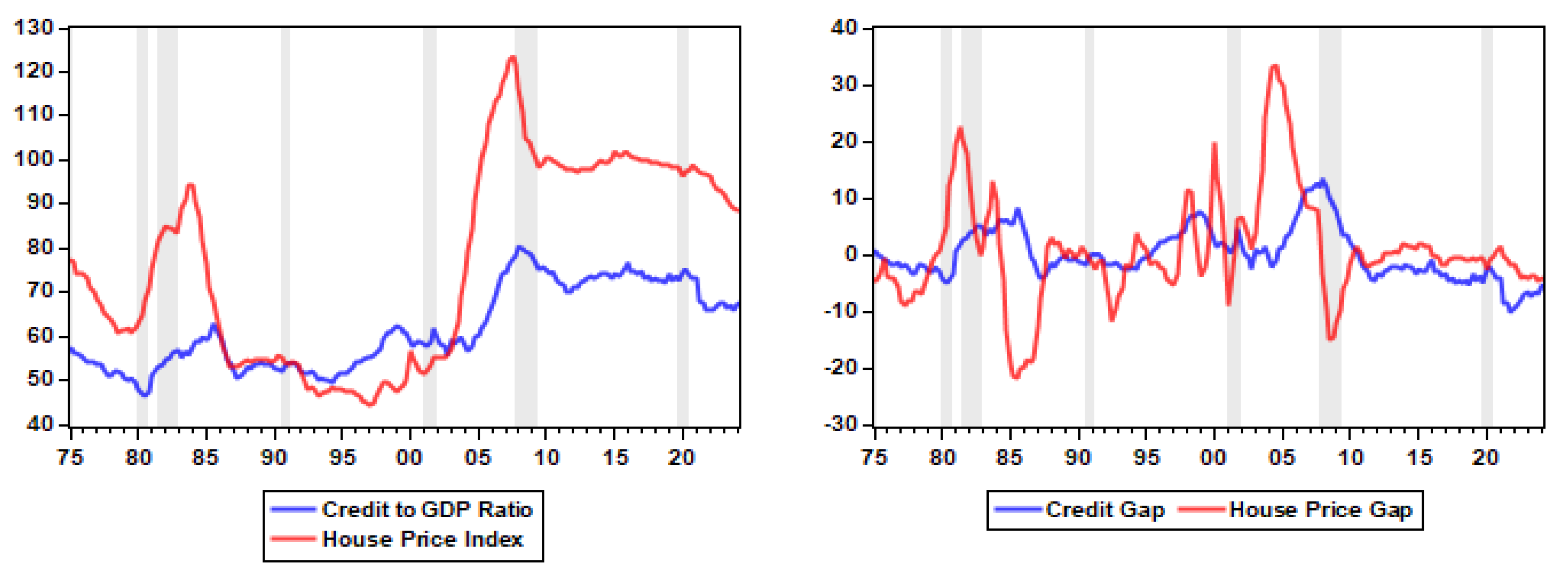
Figure 2.
Evolution of the financial cycle and the FCVIX. Source: Own estimates.
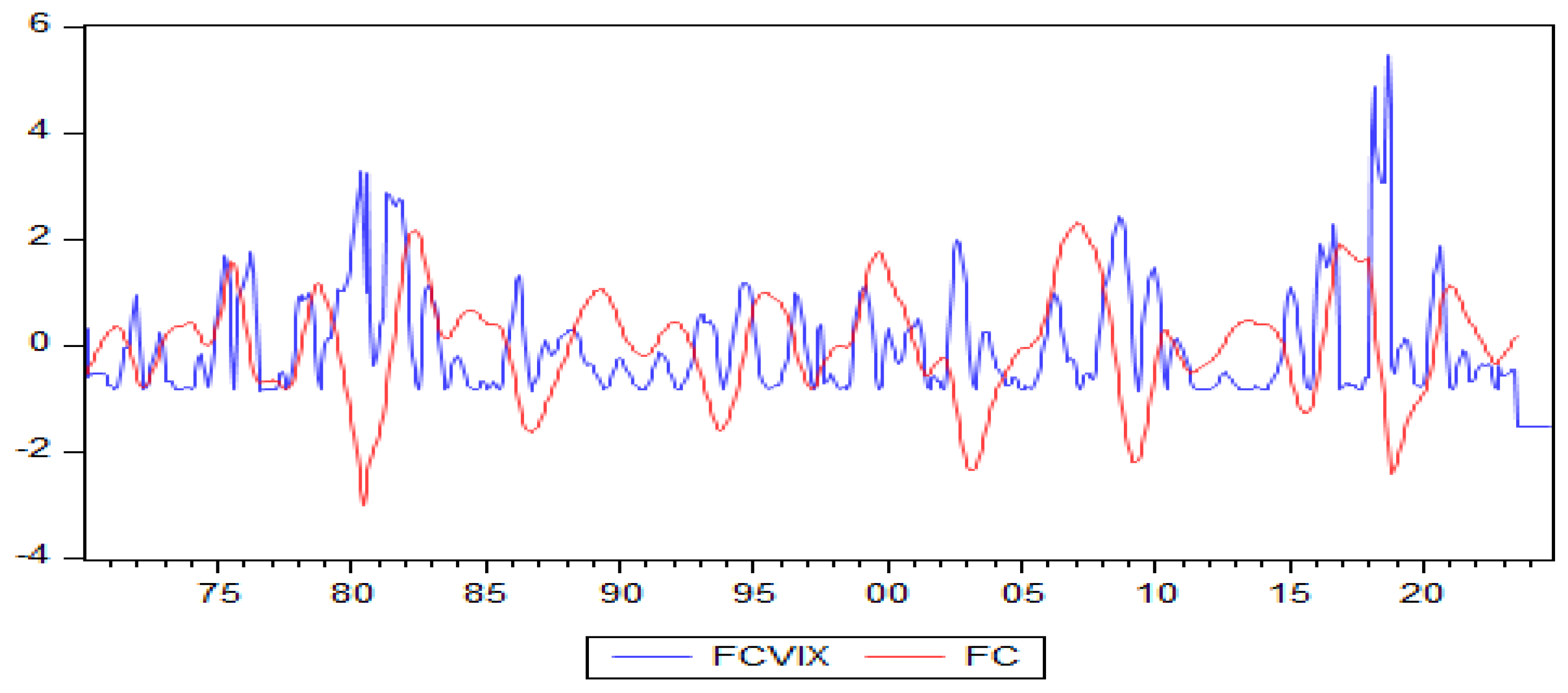
Figure 3.
Cross-correlogram of the financial cycle and the FCVIX. Source: Own estimates.
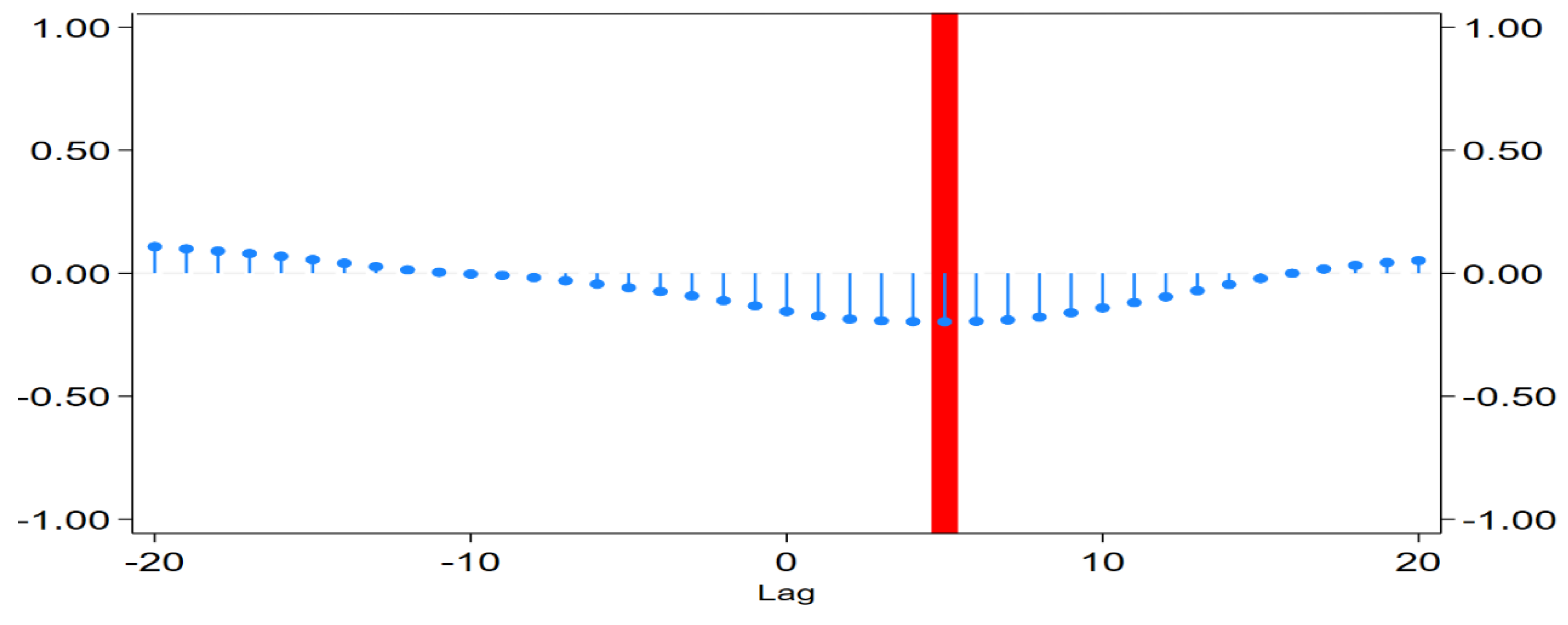

Table 1.
ADF unit roots test.
| At Level | |||||||
| FCVIX | FC | ER | Y | CPI | PR | MPI | |
| t-Statistic | -8.196 | -6.142 | -6.189 | -4.740 | -10.420 | -9.0567 | -4.367 |
| Prob. | 0.000 | 0.000 | 0.000 | 0.000 | 0.000 | 0.0000 | 0.000 |
| *** | *** | *** | *** | *** | *** | *** | |
| At First Difference | |||||||
| d(FCVIX) | d(FC) | d(ER) | d(Y) | d(CPI) | d(PR) | d(MPI) | |
| t-Statistic | -13.363 | -8.398 | -10.811 | -11.114 | -13.772 | -20.253 | -11.346 |
| Prob. | 0.000 | 0.000 | 0.000 | 0.000 | 0.000 | 0.000 | 0.000 |
| *** | *** | *** | *** | *** | *** | *** | |
Sources: Own estimates. Notes: (*) Significant at the 10%; (**) Significant at the 5%; (***) Significant at the 1% and (no) Not Significant; Lag Length based on SIC; Probability based on MacKinnon (1996) one-sided p-values.
Table 2.
MSAR main results.
| Instability state | Stability state | |||
| Coefficient | P>z | Coefficient | P>z | |
| 0.013 | 0.004 | 0.155 | 0.000 | |
| 0.009 | 0.000 | -0.010 | 0.281 | |
| -0.029 | 0.159 | 0.753 | 0.001 | |
| -0.008 | 0.168 | -0.011 | 0.056 | |
| 0.008 | 0.020 | 0.059 | 0.128 | |
| 0.019 | 0.082 | 0.250 | 0.002 | |
| 0.015 | 0.000 | 0.010 | 0.000 | |
| 0.974 | 0.000 | |||
| 0.822 | 0.000 | |||
Source: Own estimates. Notes: P>z refers to p-values.
Table 3.
Features of the FCVIX in different states.
| Instability | Stability | |
| σ | 0.001 | 0.013 |
| 28.113 | 19.837 | |
| 0.964 | 0.739 | |
| 0.036 | 0.261 |
Source: Own estimates. Notes: and refers to the probability of remaining and switching between states respectively. refer to duration of each state whereas is the variance of each state.
Disclaimer/Publisher’s Note: The statements, opinions and data contained in all publications are solely those of the individual author(s) and contributor(s) and not of MDPI and/or the editor(s). MDPI and/or the editor(s) disclaim responsibility for any injury to people or property resulting from any ideas, methods, instructions or products referred to in the content. |
© 2024 by the authors. Licensee MDPI, Basel, Switzerland. This article is an open access article distributed under the terms and conditions of the Creative Commons Attribution (CC BY) license (http://creativecommons.org/licenses/by/4.0/).
Copyright: This open access article is published under a Creative Commons CC BY 4.0 license, which permit the free download, distribution, and reuse, provided that the author and preprint are cited in any reuse.


