
Submitted:
29 January 2025
Posted:
30 January 2025
You are already at the latest version
Abstract
Countries such as Advanced Systemic Economies (ASEs) and Systemic Middle-Income Countries (SMICs) considering macroprudential policy coordination must ensure that their financial cycles are sufficiently synchronized. However, differences in the features and significance of financial cycles between ASEs and SMICs pose challenges in determining the extent of their synchronization. Accordingly, this study assesses whether a common financial cycle exists between these economies. The point of departure for this analysis is to examine the characteristics of the common financial cycle. To this end, the study employs data on capital flows, credit, house prices, share prices, and policy rates, utilizing the Markov Switching Dynamic Regression Model and the Dynamic Factor Model to identify and analyze the cycle. The findings reveal strong evidence of a significant financial cycle, which explains 83% of the total variation across countries. This cycle is characterized by longer durations compared to domestic financial cycles and occurs less frequently than domestic cycles. Moreover, it exhibits high persistence in its contractionary and expansionary phases, with greater volatility in the contractionary phase. Based on these findings, it is recommended that ASEs and SMICs consider establishing a supranational prudential authority to coordinate and oversee macroprudential policy on behalf of the majority. Such an entity should play a proactive role, particularly during contractionary phases, to mitigate systemic risks and enhance financial stability across these interconnected economies.
Keywords:
Financial cycles
; synchronization
; macroprudential policy
; policy coordination
1. Introduction
In recent years, scholars and policymakers have increasingly recognized that effective macroprudential policy implementation requires supranational prudential authorities to coordinate and supervise these policies on behalf of member states (Bassani, 2020; Valieva, 2023; Maddaloni & Scopelliti, 2022). This shift is driven by two key factors. First, national authorities tend to focus narrowly on mitigating domestic financial threats, often neglecting the broader impact of their policies on other countries (Agenor & Pereria da Silva, 2018). Second, tightening macroprudential policies in one jurisdiction can prompt financial institutions to relocate their activities to jurisdictions with more accommodative regulations, which in turn heightens risks in recipient economies (Kang et al., 2017). These dynamics create the potential for "regulatory wars," where conflicting national policies exacerbate global financial vulnerabilities and necessitate a coordinated international response. Cross-macroprudential policy coordination refers to policy actions agreed upon and taken by groups of policymakers or multilateral institutions to achieve beneficial outcomes for the international community (Agenor & Pereria da Silva, 2018). It involves relinquishing the autonomy of policymakers to use their policies to a supranational prudential authority that supervises the implementation of macroprudential policies. Moreover, cross-country macroprudential coordination is distinct from policy cooperation. The latter refers to collaboration through sharing information discussion (Portes et al., 2020)
In recent years, there has been a rise in institutions designed to mitigate challenges posed by self-oriented macroprudential policies. Examples include entities such as the International Monetary Fund (IMF), the G20, and the Bank for International Settlements (BIS) (Forbes, 2021). The IMF’s Financial Sector Assessment Program (FSAP) offers critical country-specific evaluations to identify systemic risks and recommend macroprudential tools (Towe, 2024). Similarly, the G20 has championed initiatives such as the Basel III framework and the Financial Stability Board (FSB) to align financial regulations and mitigate cross-border spillovers (Ray et al., 2023). Through its Basel Committee on Banking Supervision, the BIS has established globally recognized regulatory standards like Basel III to enhance financial stability (Basel Committee on Banking Supervision, 2011). At the regional level, organizations such as the European Union’s European Systemic Risk Board (ESRB) and frameworks like ASEAN+3 in Asia further underscore the trend toward collective action in macroprudential policy (Myklebust, 2023; Aizenman, 2022). These efforts reflect an emerging consensus on the need for coordinated and supranational approaches to safeguard global financial stability and address systemic risks effectively.
The establishment of supranational prudential bodies at the international level has prompted policymakers in Advanced Systemic Economies (ASEs) and Systemic Middle-Income Countries (SMICs) to advocate for the creation of their own regional supranational prudential authorities (Agenor & Pereria da Silva, 2018). The advanced systemic economies refer to the United States (US), the United Kingdom (UK), Japan (JPN), and Germany (DEU) (Adarov, 2022). The systemic middle-income countries refer to Brazil (BRA), China (CHN), India (IND), Indonesia (IDN), Mexico (MEX), Russia (RUS), Turkey (TUR), and South Africa (ZAF) (Agenor & Pereria da Silva, 2018). First, this push is primarily driven by the observation that macroprudential policy coordination efforts led by major institutions, such as the IMF and the BIS, tend to disproportionately benefit countries where financial crises originate (Agenor et al., 2024). At the same time, the costs of such coordination efforts from large supranational prudential bodies are distributed equally among all participating nations, resulting in concerns over inequitable burden-sharing (Kranke & Yarrow, 2018). Second, these economies play a critical role in the global financial system, collectively accounting for a significant share of world GDP—ranging from 73.8% in the 1990s to 67% in recent years (World Bank, 2023). As a result, increasing policy coordination between these economies will further consolidate their economic position, enhancing their collective ability to influence and stabilize the global financial architecture.
Another key motivation arises from these economies' adverse effects on the rest of the world. Financial volatility within ASEs and SMICs has had far-reaching global repercussions, as seen during the 2007–2009 global financial crisis and the European debt crisis (Zaspel, 2021). Studies highlight that financial market fluctuations driven by changes in these economies accounted for 50% to 80% of the variations observed in other economies (Agenor & Pereira da Silva, 2023). Moreover, when these economies implement tighter financial regulations, capital flows often shift to less regulated jurisdictions, amplifying systemic risks globally (Chari et al., 2023). Such spillovers underscore the need for greater accountability in these economies' macroprudential policymaking. Coordinated efforts would compel them to consider the potential adverse effects of financial and regulatory spillovers when calibrating macroprudential policies. Policymakers argue that establishing a coordinated macroprudential framework could mitigate these spillovers and strengthen global financial stability.
Financial cycle synchronization, underpinned by increasing financial integration, is a prerequisite for establishing a supranational prudential authority (Gammadigbe, 2022). Financial integration promotes international risk-sharing by enabling financial flows to stabilize economies during downturns; for example, inflows from resilient foreign counterparts can buffer consumption and output during domestic slumps (Stoica et al., 2020). However, integration also amplifies vulnerabilities, as crises in one country can trigger rapid outflows and cascading disruptions across borders (Barro & Bassolet, 2023). Moreover, the synchronization of financial cycles is critical because divergent cycles lead to conflicting macroprudential policy preferences (Akhmetov et al., 2021). Countries in an expansionary phase of their financial cycles would advocate for tighter macroprudential measures to mitigate risks. In contrast, those in a contractionary phase would push for easing policies to support recovery. Without synchronization, such conflicting preferences hinder coordinated policy efforts. Thus, cross-country macroprudential policy coordination becomes essential—not only to manage systemic risks and enhance the benefits of integration but also to reconcile policy priorities and align disconnected economies for shared financial stability.
Existing studies on the synchronization of financial cycles in systemic economies reveal a lack of consensus, reflecting the complexity of these dynamics and their implications for policy coordination. Some studies emphasize significant differences between the financial cycles. For instance, financial cycles in ASEs tend to be longer and more pronounced compared to those in SMICs (Adarov, 2022; Schuler et al., 2020; Bai et al., 2019). The former are primarily driven by internal factors, such as the level of financial development, while the latter are more heavily influenced by external factors, including shifts in policy rates and credit conditions in advanced economies (Chorafas, 2015; Aldasoro et al., 2020). Additionally, the spillover effects of financial cycle shocks from ASEs to SMICs are significantly stronger than the reverse, highlighting an asymmetrical relationship in spillover dynamics (Liu et al., 2020; Ha et al., 2020; Tian, 2024). Conversely, other studies point to important similarities between the two groups. Both ASEs and SMICs drive global output gaps, and their financial cycles frequently peak during periods of international crises (Grintzalis et al., 2017; Guillochon & Le Roux, 2023). This dual role as triggers and amplifiers of global financial instability underscores the interconnectedness of their financial systems (Laxton et al., 2019; Furlanetto et al., 2021). These shared vulnerabilities suggest a degree of alignment in how their financial cycles respond to systemic shocks.
The divergence in findings carries significant implications for coordination. If financial cycles are poorly synchronized, attempts to establish a supranational prudential authority may face challenges in aligning macroprudential policies, as disparate cycles would require tailored interventions that may conflict across regions. On the other hand, evidence of synchronization strengthens the case for coordination, as it implies that shared policies could effectively mitigate systemic risks across both groups. Moreover, the asymmetrical spillover effects highlight a potential source of tension, as ASEs may disproportionately benefit from coordinated efforts, while SMICs bear a larger share of the spillover burden. Addressing these competing implications is critical to assessing the feasibility and effectiveness of a coordinated macroprudential framework, as synchronization—or the lack thereof—directly shapes the operational design and governance of such initiatives.
Acknowledging the complexities arising from the differences and similarities in the financial cycles of ASEs and SMICs, this study aims to evaluate the existence of a common financial cycle between these two groups of economies. To this end, the study utilizes the Markov Switching Dynamic Factor Regression model to construct and rigorously analyze the key features of the shared financial cycle. The analysis spans the period from 1960 to 2022, using high-frequency monthly data on indices of house prices, capital flows, domestic credit, share prices, and policy rates. The structure of the study is as follows: Section 2 provides a comprehensive review of the relevant literature, situating the study within the broader context of financial cycle research. Section 3 details the data sources and methodological approach employed in the analysis. Section 4 presents the empirical findings and critically discusses their implications. Finally, Section 5 concludes by summarizing the key insights and outlining directions for future research.
2. Literature Review
The theoretical exploration of financial cycles and their synchronization across nations has been underpinned by several robust conceptual frameworks. Among these, the financial trilemma framework emerges as a key theoretical construct, highlighting the inherent tension between achieving three critical objectives: financial integration, autonomous financial policymaking, and financial stability (Obstfeld, 2021; Aizenman, 2019; Cimoli et al., 2020). This framework posits that it is impossible for a nation to simultaneously achieve all three objectives, necessitating trade-offs in policy decisions. For instance, countries prioritizing financial stability and autonomy may have to forgo full financial integration. In this scenario, countries may face international pressure to insulate their economies from external financial shocks and policy spillovers, potentially triggering regulatory competition—or even "regulatory wars"—as nations adopt unilateral measures to shield their financial systems (Ligonniere, 2018). This tension arises because financial integration enhances capital mobility and economic efficiency and exposes domestic economies to volatility from external developments (Tang & Yao, 2022). As a result, countries prioritizing financial stability and autonomy may be compelled to limit full financial integration to mitigate these risks. However, ex-ante macroprudential policy offers a potential solution by proactively addressing systemic vulnerabilities before they materialize (Agenor et al., 2023). Instead of resorting to reactive, uncoordinated regulatory interventions, which may exacerbate market fragmentation, macroprudential coordination can help align financial stability objectives across jurisdictions. This has led to the growing importance of cross-country collaboration in macroprudential policymaking, particularly among economies with deeply interconnected financial markets (Agenor et al., 2024). By fostering a cooperative approach, coordinated macroprudential policies can mitigate the risks of regulatory arbitrage, enhance financial resilience, and promote stability without undermining the benefits of financial integration (Liu & Zhang, 2023).
Another widely referenced framework is the push-pull model, which explains the dynamics of global capital flows and financial cycle synchronization (Urbanski, 2022; Mudyazvivi, 2018; Ashenafi & Dong, 2023; Ramesh & SriRam, 2023). Push factors, such as global interest rates and financial conditions in advanced economies ASEs, exert external pressures that drive capital flows in emerging markets. When interest rates in ASEs are low, investors seek higher returns in emerging markets, leading to increased capital inflows (Carstens & Freybote, 2020). Conversely, when financial conditions tighten—such as during monetary policy normalization or risk-off episodes—capital reverses, triggering financial instability in emerging economies (Sahoo et al., 2020). These external pressures, driven by macroeconomic policies in ASEs, highlight the importance of macroprudential measures in recipient countries to mitigate volatility and enhance financial resilience. Pull factors attract capital inflows based on a country's internal economic conditions rather than external pressures. SMICs, factors such as strong economic growth, sound monetary policies, stable inflation, and well-regulated financial markets enhance investor confidence, making these economies more appealing investment destinations (Fiandy & Saadah, 2024; Kang & Kim, 2019). For instance, if an SMIC maintains low inflation and credible monetary policy, it signals economic stability, encouraging long-term foreign investment. Similarly, robust financial markets with high liquidity and strong institutions reduce investment risks, attracting capital even when global financial conditions tighten. Thus, while push factors create external pressures, pull factors determine a country's ability to sustain capital inflows and minimize the risks of sudden reversals. The push-pull framework elucidates the dual influence of global and domestic factors in shaping financial cycle synchronization, highlighting the asymmetric vulnerabilities of economies to external shocks.
The synchronization of financial cycles within ASEs has been a focal point of financial literature, emphasizing the role of global factors in aligning credit, housing, and equity markets. Studies reveal that financial cycles in these economies are increasingly synchronized due to shared monetary regimes, financial liberalization, and globalization (Adarov, 2022; Winter & Koopman, 2022). For instance, Skare & Porada-Rochon (2020) found that financial cycles in Germany, the US, and the Netherlands initially displayed shorter durations and lower amplitudes compared to France, Italy, and Spain. However, following financial liberalization in the mid-1980s, these cycles became increasingly aligned, reflecting the homogenizing influence of global market forces. The synchronization is also evident in the spillover effects of monetary policies. Degasperi et al. (2020) finds that US interest rate changes significantly influence global financial conditions by affecting capital flows, leverage cycles, and risk-taking behavior. Obstfeld (2019) show that US monetary policy shocks tighten financial conditions in other advanced economies, particularly in the Eurozone, leading to slower credit growth and asset price declines. Miranda-Agrippino and Rey (2021) further demonstrate that the global financial cycle amplifies these effects, with US monetary easing driving synchronized credit expansions and tightening causing simultaneous contractions. The VIX, a widely recognized measure of market uncertainty and risk aversion, has been identified as a critical global factor influencing ASE financial cycles. Miranda-Agrippino and Rey (2021) demonstrated that lower volatility levels correspond to increased capital flows, amplified credit growth, and asset price booms across ASEs. This co-movement underscores the growing interconnectedness of financial markets in advanced economies and the critical role of global monetary policy in shaping financial dynamics.
The interplay between ASEs and SMICs adds another layer of complexity to the synchronization of financial cycles. Studies indicate that SMICs are particularly vulnerable to external shocks originating in ASEs due to their dependence on global capital flows and limited financial resilience. For example, Morelli et al. (2022) highlighted how global banks act as conduits for transmitting monetary conditions from ASEs to SMICs. Easing financial conditions in advanced economies often result in capital inflows to SMICs, leading to credit booms and increased financial vulnerability. Empirical evidence also points to the asymmetric nature of synchronization. Di Giovani et al. (2022) found that the global financial cycle, driven by factors such as the VIX and US monetary policy, significantly impacts SMICs by lowering borrowing costs and increasing local lending. However, these effects are amplified by the weaker regulatory frameworks and higher exposure of SMICs to global banks. Similarly, Gomez-Pineda (2020) emphasized that global uncertainty and risk aversion are primary drivers of financial cycle volatility in SMICs, further reinforcing the need for enhanced macroprudential policy coordination between ASEs and emerging markets. This dynamic underscores the bidirectional nature of influence, where shocks in SMICs, although less frequent, can also reverberate across global financial markets.
Empirical studies have employed various econometric techniques to explore the attributes and synchronization of financial cycles. Schuler et al. (2020) used spectral density analysis to demonstrate that financial cycles in advanced economies are longer and exhibit greater amplitudes compared to business cycles. Similarly, Drehmann et al. (2012), using the SBBQ dating algorithm, found that credit and housing market cycles tend to be more synchronized within countries but exhibit significant cross-country differences. For instance, financial cycles in Germany, characterized by shorter durations and lower amplitudes, are less synchronized with those in Japan, which exhibit longer and more pronounced cycles (Schuler et al., 2017). Beyond advanced economies, emerging markets exhibit a more pronounced sensitivity to global factors, as seen in studies by Gomez-Gonzalez et al. (2015), where credit and GDP cycles demonstrated strong correlations at medium- to long-term frequencies. These findings illustrate the global interconnectedness of financial cycles while highlighting regional cycle amplitude and duration disparities.
Despite these differences, the increasing synchronization of financial cycles has important implications for macroprudential policy coordination. Studies such as Adarov (2022), Berge & Hienzsch (2024), and Potjagailo Wolters (2023) emphasize the role of common factors, such as global risk sentiment and monetary policies, in driving financial cycle synchronization. These commonalities suggest that coordinated policy measures can mitigate the adverse effects of synchronized cycles while preserving the benefits of financial integration. However, such coordination is not without its challenges. Divergent financial regimes, varying levels of financial development, and differing policy priorities often hinder efforts to implement cohesive macroprudential strategies. Furthermore, sudden stops, characterized by abrupt reversals of capital inflows, pose a significant threat to financial stability in SMICs and emphasize the need for resilience-building measures.
The synchronization of financial cycles across ASEs and SMICs underscores the need for coordinated macroprudential policies to address shared vulnerabilities and enhance financial stability. Agenor and Pereira da Silva (2022) argue that countries with highly synchronized financial cycles benefit from harmonized regulatory frameworks, reciprocal macroprudential measures, and coordinated responses to global shocks. For instance, countercyclical capital buffers and international liquidity support mechanisms can help mitigate the procyclical effects of global financial cycles and reduce systemic risks. Flexible exchange rates and robust fiscal policies have also been suggested as buffers against the adverse effects of synchronized cycles (Cavallo & Frankel, 2008). However, achieving effective policy coordination remains challenging due to differences in financial structures, regulatory regimes, and economic priorities. Galati et al. (2016) and Runstler and Vlekke (2018) noted that countries with heterogeneous financial cycles often face difficulties aligning policy objectives, particularly when distinct domestic factors drive their cycles. These differences highlight the necessity of a tailored approach that considers national circumstances while leveraging global cooperation.
Despite the breadth of research on financial cycles, significant gaps remain. Notably, the literature reveals that different variables produce varying results in identifying and characterizing financial cycles. These discrepancies stem from differences in methodologies, country-specific factors, and the selection of variables such as policy rates, credit, house prices, share prices, and capital flows. Addressing this inconsistency is essential for advancing our understanding of financial cycle dynamics. The present study aims to fill this gap by examining whether there is a common financial cycle in both ASEs and SMICs. The central hypotheses are as follows: (1) there exists a common financial cycle across ASEs and SMICs, (2) policy rates, credit, house prices, share prices, and capital flows are key drivers of the common cycle, and (3) the common cycle is long in duration and exhibits greater amplitude. The null and alternative versions of these hypotheses are:
H0: There is no common financial cycle across ASEs and SMICs.
H1: There is a common financial cycle across ASEs and SMICs.
H0: Policy rates, credit, house prices, share prices, and capital flows do not drive the common financial cycle.
H1: Policy rates, credit, house prices, share prices, and capital flows drive the common financial cycle.
H0: The common financial cycle is not long in duration and does not exhibit greater amplitude.
H1: The common financial cycle is long in duration and exhibits greater amplitude.
By testing these hypotheses, this study seeks to provide a unified framework for understanding financial cycle synchronization and its drivers, bridging the gaps in existing literature and offering insights for more effective macroprudential policy coordination.
3. Data and methodology
Finally, the data used to construct the common financial cycle is presented. The sample is made up of twelve countries: Brazil, China, Germany, India, Indonesia, Japan, Mexico, Russia, Turkey, the United Kingdom, the United States, and South Africa. It covers the period 1960m1 – 2022m12. In order to capture various aspects of international risk, the chapter uses six key indices, each constructed through principal component analysis. Table 1 summarizes these indices. These six indices constitute the ASEs and SMICs' Common Financial Cycle. They are the Central Bank Policy Rates Index (PR), Property Prices Index (PP), Share Prices Index (SP), VIX measure of uncertainty, capital flows Index (CP), and Domestic Credit Index (CR). The central bank policy rates indices include eleven central bank rates, which are the prime loan rate (Brazil), the official repo rate (United Kingdom), the official base rate (Indonesia), the repo rate (India), the short-term policy interest rate (Japan), overnight money-market rate (Mexico), official refinancing rate (Russia), official week rate (Turkey), federal reserve target (United States), and the official repo rate (South Africa). These central bank policy rates were collected from the Bank of International Settlements (BIS) Other Indicators Statistics. The property prices index represents the housing markets and includes the real house price index for each country. The real house price index is the ratio of the nominal house price index to the consumer’s expenditure deflator in each country in the sample. Therefore, the property prices index comprises twelve real house price indexes.
The index for share prices represents the equity markets. It comprises prices of common shares of companies traded on domestic or foreign stock exchanges for each of the twelve countries in the sample. The real house price indexes and share prices were both collected from the OECD’s Macroeconomic Indicators Database. Conversely, the VIX was collected from the Chicago Board Options Exchange (CBOE) and used in this chapter to capture global financial markets' risk and uncertainty. The credit index is used to represent the credit market of each country. In each country, the credit index comprises credit from all sectors to the private non-financial sector as a percentage of GDP. Data pertaining to credit for each country were collected from the BIS Credit Statistics. Finally, the capital flows index includes, for each country, net borrowing/lending balance in the financial account, foreign direct investment, net acquisition of assets, equity, and investment fund shares. Each variable was sourced from the IMF International Financial Statistics.
The common approach in deriving these indices is to combine all the variables into a single index representing the indices. That means that the policy rates index is constructed by combining the eleven central bank policy rates into one index. The property price index is constructed by combining the twelve real house indices into one index. The procedure is used to obtain the credit, capital flows, and share price indices. Various methodologies exist in the literature to assist with this process, including spectral analysis (Strohsal et al., 2019), dynamic factor modeling (Adarov, 2022), and principal components analysis (PCA) (Brave & Butters, 2011; Eickmeir et al., 2014). Amongst these methodologies, the chief advantage of PCA is that it reduces the curse of dimensionality in the dataset and only focuses on the most relevant features describing the co-movement of variables (Stock and Watson, 2010). Consequently, this study follows Brave and Butters (2011) and employs the PCA to construct the financial cycle.
The study is interested in the covariances, variances, and correlation of all the variables making up each index. The information contained in these variances, covariances, and correlations is crucial to formulating the financial cycle. The first step is to look for a linear function, , Of the elements of, x = 3 financial indicators having maximum variance. Where, a1 is a vector of p variables such that, a11, a12..., a1p, and denotes transpose, such that:
1
Afterwards, one can look for a linear function, , uncorrelated with, and having maximum variance, such that at the kth stage a linear function of, with maximum variance exists and is uncorrelated with, . The kth derived variable, , is one of the derived principal components (PCs) explaining variations in the variables. There can be more than one PCs. However, for the purpose of this study, we focus on the PC that explains the most common variations of the variables. The study refers to these components as the policy rate index, property prices index, share prices index, credit index, and capital flows index, as described above.
Contrary to the methodological approaches mainly adopted to measure financial cycles in a country (Bosch and Koch, 2020), it has been demonstrated that a Markov Switching Dynamic Factor model could be another suitable method for analysing financial cycles Nyati et al. (2021). The model assumes that the growth rate of economic cycles has two stages: the downturn and the upturn (Nyati et al., 2021). The cyclical behaviour of economic cycles can be represented by an unobservable factor extracted from the combination of the six indices above. Moreover, the switch from a downturn to an upturn, and vice-versa, is assumed to occur instantaneously with no transition periods. According to Nyati et al. (2021) transition period before a deep crisis is usually enough to be omitted, which provides motivation for assuming instantaneous transition (Doz & Petronevich, 2020). Accordingly, the study employs the model to construct and characterize the ASEs’ and SMICs’ Common Financial Cycle (ASCFC).
The model is divided into equations: one representing the factor model and the other defining a Markov Switching model, which was assumed for the common factor. The first two equations show each series of the information set decomposed into the sum of a common component and an idiosyncratic component as follows:
(2)
(3)
Equations 2 and 3 above are known as the Dynamic Factor Model (DFM), where is a vector of the six indices, is a common univariate factor representing ASCFC, and are vector of idiosyncratic factors, which are uncorrelated with as all leads and lags, is an vector of factor loadings. One requirement from this equation is for all variables to be stationary, i.e., some variables will appear as the first differences of non-stationary indices.
The third and fourth equations define a Markov switching model of Hamilton (1989). The model could mark time, in terms of his method, as a latent random variable, governs the state or regime with denoting low or negative growth rate, and =1 denoting a high or positive growth rate. Two states, signifying positive and negative growth rates, are adequate to mark turning points since indicates a downturn and indicates an upturn (Bosch & Ruch, 2013). Consider the development of an index , where which is characterized by two states as follows:
(4)
(5)
Where and are state-dependent means in state one and state two, respectively. The two states model shifts in state-dependent mean, and it is unknown which state the process is in, therefore, the state variable is unobserved. Markov Switching regression models allow the parameters of the state-dependent means to vary over the unobserved state. In the simplest case, this model can be expressed as a Markov Switching Dynamic Regression (MSDR) with a state-dependent mean. MSDR models allow a rapid adjustment after the process changes state. These models are often used to model monthly or higher-frequency data. When the process is in state time , a general specification of the MSD model is written as
(6)
Where is the dependent variable, is the state-dependent mean, is a vector of exogenous variables with state-invariant parameters, is a vector of exogenous variables with state-dependent parameters and is an independent and identically distributed (i.i.d) normal error with mean zero and state-dependent variance and may contain lags of . MSDR models allow states to switch according to a Markov switching process. This chapter adopted a two-state MSDR model to conform to the growth rate cycle downturns and upturns of the ASEs and SMICs Common Financial Cycle. Consequently, equation 3.10 above is written as follows:
(7)
The transition probabilities of a change in a state from state to state are summarised with the use of a transition matrix, namely, for the two-state Markov chain as follows:
(8)
Where, , meaning that the probability that the current state is given the previous state was . In order to be able to estimate the coefficients for the above equation, one has to maximize the log-likelihood of the unconditional density function . To identify the ASEs and SMICs Common Cycle Turning Points, the filtered probabilities were calculated based on the information available until (Doz and Petronevich, 2016).
The model proceeds in three steps as follows:
The initial step involves the extraction of a common factor from an amalgamation of a large set of variables, as suggested by recent literature (see Chorafas, 2015; Kota and Goxha, 2019). A dynamic factor model in state space was adopted in this context. The DFM specified in equation 3.11 is written as a linear state-space model. Let be the degree of the lag polynomial matrix let denote an vector, and le where is the of coefficients on the lag in . Also, let (L) be the matrix consisting of 1’s and 0’s and the elements of such that the static model in equations 2 and 7 is rewritten in terms of :
(9)
(10)
Where is a matrix of 1’s and 0’s selected so that equation 6 and equation 7 are the same. Furthermore, is assumed that following the following process:
(11)
With the assumption that is independent and indirectly distributed, and is independent and indirectly distributed, and and are independent. Given these parameters, the Kalman filter can be used to compute the maximum likelihood and to estimate the filtered values of and . The Kalman filter is a recursive process constructed on the error and the factor matrix over time. This is done by systematically updating the mean’s conditional distribution ) and the conditional distribution of variances depicted in the following process as shown in the paper by Katzfuss (2016):
(12)
(13)
(14)
(15)
Where is a probabilistic time-varying matrix, and is a probabilistic time0varying matric, these are also known as transition matrices. The filters estimate of is depicted in terms of and is the one-period ahead forecast of shows the covariance matric of each corresponding predicted value . This recursive process allows the coefficient estimation of and through the likelihood function inbuilt into the Kalman filter (Harvey, 1990).
After producing a dynamic common factor, the study will use the CF (Christiano-Fitzgerald) filter, HP (Hodrick-Prescott) filter, and BK (Baxter-King) filter to detrend the factor and isolate the ASE-SMIC Common Financial Cycle (ASCFC). Each of these filters offers distinct advantages for analyzing financial cycle dynamics. The CF filter is particularly advantageous for capturing the cyclical component in data with irregular or asymmetric fluctuations. This filter allows for more flexibility in dealing with high-frequency noise often present in financial time series data. By employing this filter, the study can better account for both short- and long-term cyclical movements, making it useful for financial data that may exhibit complex and varying patterns over time (Christiano & Fitzgerald, 2003).
The HP filter is widely used for extracting long-term trends from time series data, making it suitable for analyzing financial cycles with a clear distinction between trend and cyclical components. This filter is effective in smoothing out short-term fluctuations and focusing on the underlying financial cycle. However, it has the disadvantage of potentially over-smoothing during periods of short-term volatility, which may distort the analysis of financial cycles in more volatile environments (Hodrick & Prescott, 1997). Despite this, it remains a standard tool in financial cycle analysis due to its simplicity and broad applicability. The BK filter is particularly beneficial when a study requires a focus on business-cycle frequency fluctuations. It is designed to extract cyclical components within a specified frequency range, which makes it especially effective for isolating medium-term cycles that are crucial for macroeconomic and financial stability analysis (Baxter & King, 1999). The BK filter is often preferred for its ability to minimize the bias associated with endpoints, which can be problematic in time series analysis, especially when dealing with limited sample sizes or data that spans fewer periods.
By applying all three filters, the study can take advantage of each method's strengths to detrend the dynamic common factor and derive a more robust measure of the ASCFC, providing a comprehensive view of the synchronized financial cycles between ASEs and SMICs. The use of multiple filters ensures that the analysis captures the most relevant cyclical dynamics while mitigating the potential weaknesses of any single method.
The third step estimates maximum likelihood, the parameters of a Markov Switching Dynamic Regression Model. The aim is to fit a univariate model as in (Hamilton, 1989) to the estimated factor which is taken as if it were an observed variable. In order to identify the ASEs and SMICs Common Financial Cycle turning points, the study follows the footsteps of Nyati et al. (2021). A peak in the ASCFC in period is identified if financial activity was in an upturn in period and filtered probability and a trough is defined in period if financial activity was on downturn in period and the filtered probability .
4. Results and Discussion
4.1. Preliminary results
The Principal Common Analysis (PCA) was used to extract a common factor from the indexes of the policy rates (PR), property prices (PP), credit (CR), capital flows (CP), share prices (SP) and the VIX. This common factor is here referred to as the ASE and SMICS Common Financial Cycle (ASCFC). Table 2 depicts the factor loadings of the top six factors, F1 through to F6, identified by the PCA. According to Stock and Watson (2011), only factors with an eigenvalue larger than one should be considered. Therefore, given the results in Table2, only the first factor, F1, represents the ASEs and SMICs Common Financial Cycle. As shown in Table1, F1 explains 83 percent of all variations in the variables, whereas other factors explain less than 11 percent combined. This perennial finding indicates the existence of a common financial cycle between ASEs and SMICs and is supported by a growing body of empirical research. Miranda-Agrippino and Rey (2021) provide evidence that global financial conditions, largely shaped by US monetary policy, drive synchronized credit expansions and contractions across economies, reinforcing the idea of common financial cycles. Expanding on this, Beirne (2020) identifies a regional credit cycle among advanced economies, while distinct asset price cycles exist in Asia, Eastern Europe, and Latin America, suggesting that financial cycle co-movements can manifest at both global and regional levels. Similarly, Lv et al. (2023) find that the persistence and mean of aggregate financial cycles are aligned across both developing and developed regions, further supporting the existence of a common financial cycle. Additionally, Jordà et al. (2018) provide evidence of a regional financial cycle in equity prices among advanced economies, highlighting that financial cycles are not only globally synchronized but also exhibit strong regional dynamics. Agenor and Pereira da Silva (2023) further demonstrate that financial fluctuations in ASEs account for a substantial portion of volatility in SMICs, confirming the transmission of financial cycle shocks across different economic groups.
According to Brooks (2019), a factor loading between 0.4 and 0.75 in absolute terms indicates that a variable corresponds moderately well with the underlying common factor. Furthermore, any loading parameter larger than 0,75 indicates a strong correspondence between the underlying common factor and a variable (Brooks, 2019). From Table 3, it can be deduced that property and share prices have the highest factor loadings and contribute the most towards the ASCFC. Hence, according to the results, asset prices are the strongest underlying drivers of the ASCFC. This is followed by credit, and capital flows with factor loadings of 0,93 (93%) each. Hence, credit and capital flows are another significant driver of the ASCFC.
The ASEs and SMICs index for policy rates has a positive loading of 0,88. This suggests a positive relationship exists between monetary policies and the ASEs and SMICs' Common Financial Cycles. This positive link can be associated with the monetary policy puzzle. The monetary policy puzzle occurs when interest rates increase in response to higher inflation or excessive credit, and asset price growth is not enough to tame higher inflation or excessive credit and asset price growth (Bernanke, 2020). What follows is that policy rates and economic activity will expand simultaneously (Bilbiie, 2024). This results in the positive relationship between policy rates and the ASEs and SMICs Common Financial Cycle. Another example is when monetary authorities anticipate that there will be excessive credit and asset price growth in the future but delay tightening policy rates to a later stage. When policy rates are tightened later, economic activity will expand.
Figure 1 displays a time series plot of the ASEs and SMICs common factor, and a detrended version of the ASCFC obtained through the Christiano & Fitzgerald (2003) bandpass filter. Applying eyeball inspection Figure1, the ASCFC has properties of a conventional financial cycle described in Borio (2014). First, as predicted by economic theory, the ASCFC has noticeable periods of upswings and downturns (Zarnowitz, 1992; Laidler, 1999; Besomi, 2006). For example, the ASCFC was in a downturn phase following the Dot.Com Bubble in 2002. Another example is that the ASCFC was in an upswing phase before it peaked during the 2007-09 global financial crises. The upswing periods occur when favourable developments, such as strong credit growth, rising asset prices, and falling policy rates, become excessive (Nyati et al., 2021). In turn, these developments induce euphoria about the future, which causes economies to invest in riskier assets that seem safe at the time and result in financial instability (Brahim & Chaâbane, 2023). Hence, the seed for the ASCFC downturn is sown during the upturn.
Figure 1 suggests that the common financial cycle is less frequent compared to the country-specific cycle that occurs every decade (Borio, 2014). According to the figure, there are visible cycles that are two decades apart. The first began in the late 1970s and ended in the early 1980s. The second began in the late 1990s and ended in 2019. Moreover, Figure, 1suggests that the common cycle became longer and ampler over time. The first cycle lasted a decade whereas the second cycle lasted almost three decades. The first cycle peaked at 2 percent, whereas the second cycle peaked at 2 percent, thereby suggesting that the recent cycle is more ample than previous cycles. Figure 1 also displays that these cycles coincided with episodes of financial turmoil. Typical examples include the First Oil Crises (1973), Second Oil Crises (1979), Black Monday (1987), Black Wednesday (1992), Asian Financial Crises (1997), Dot.Com Bubble (2000-2002), Global Financial Crises (2007), European Sovereign Debt Crises (2010), China Stock Market Crash (2016) and Covid-19 Pandemic (2020). The second oil crisis (1979) and the Global Financial Crisis (2007) occurred at or around a peak in the ASCFC. Whereas other crises, for instance, the Euro-Debt Crisis (2010), the Chinese Stock Market Crash (2016), and Black Monday (1987) coincided with the contractionary phase of the ASFCF. Some crises, such as the Dot.Com Bubble (2002) and the Asian Financial Crisis (1997), preceded financial cycle peaks. From a point of cross-country macroprudential policy coordination, the finding that financial crises are closely associated with the ASCFC implies that this cycle can act as an early warning indicator of the build-up of systemic risk (Bierni, 2020). Hence the study proceeds to analyse the ASCFC.
4.2. Main results
Table 3 below displays the Markov chain dynamic regression model from 1960 month 1 to 2022 month 12. Firstly, consider the results from the regime-dependent means, and . The regime-dependent means of both regimes, and are statistically significant at a 99 percent confidence interval and have opposite signs. Therefore, the point estimates of the regime-dependent means are statistically different from each other. This provides evidence to earlier observations that two distinct regimes or phases can characterize the ASCFC. Other cycles in the literature also have two regimes (Layton & Katsuura, 2001; Lin & Hsiu-Hua, 2005; Botha and Saayman, 2022). Consequently, it can be expected that the ASCFC shares similar features with other financial cycles. The regime-dependent mean in regime 1, , is negative, and the regime-dependent mean in regime 2, , is positive. Given that , the evidence is provided that one can interpret regime one as the contraction phase and regime two as the expansion phase of the ASCFC (Tastan & Yildirim, 2008). Indeed, the literature has established that financial cycles are characterized by oscillations between expansions and contractions in financial activity (Borio, 2014).
Secondly, consider the variance parameters, and . Both parameters are statistically significant. is statistically significant at a 95% confidence interval whereas is statistically significant at a 99% confidence interval. In absolute terms, ; this indicates that there is volatility asymmetry between the two regimes (Li, 2010). The results show that there is more volatility during the contraction phase relative to volatility during the expansion phase. This is because the expansion phase is associated with increased financial risks such as over-borrowing, excessive credit and asset price growth, and weaker financial regulations. In contrast, during the contraction phase, there is a financial crisis, which transforms debt into higher default rates. Moreover, asset prices drop, which reduces the value of collateral, thereby leading to severe losses for lenders.
Thirdly, consider the transition matrix parameters, P11-C and P21-C. Both parameters are statistically significant at a 99 percent confidence interval and have the same sign. The positive P11-and P21-C signify that a decrease in the ASCFC is associated with higher probabilities of remaining in the contraction regime, lowering the transition probability out of regime one and increasing the transition from regime two into regime 1 (Kim & Nelson, 1999). Likewise, an increase in the ASCFC is associated with higher probabilities of remaining in the expansion regime, thereby lowering the transition probability out of regime two and increasing the transition probability from regime 1 to regime 2. These results relate to the transition probabilities which 0,93, and which 0,97. Note that provides the conditional probability of remaining in a contraction phase once in a contraction phase and provides the conditional probability of moving from a contraction to an expansion. Furthermore, provides the conditional probability of remaining in an expansion once in an expansion phase, and provides the conditional probability of moving from an expansion to a contraction. Both and are closer to one. This indicates a high probability of remaining in the contraction phase once in a contraction. There is a high probability of remaining in an expansion once in a phase. However, the probabilities also reveal that sharp asymmetries exist in the ASCFC.
According to these results, the conditional probability of moving from a contraction to an expansion, , in the ASEs and SMICs Common Financial Cycle is 6 percent, and the probability of moving from an expansion to a contraction, , is 2%. On the other hand, the probability of remaining in the contraction phase one in the contraction phase is, is 93 percent, and the probability of remaining in an expansion phase once in the expansion phase, is 97 percent. Thus, there is an asymmetrically high probability of remaining in each regime relative to the probability of moving to another regime, indicating a persistence level in each regime (Li et al., 2005). To further illustrate, Figure 2 and Figure 3 visually represent the probabilities of entering each regime.
Consider Figure2, which shows the probability of entering a contraction phase. Applying ocular econometrics to Figure 2, downturns in the ASCFC (Black line), occur around the same time as the peaks in the probability of entering a contraction phase (Blue line). Now consider Figure 3. The black line plots the ASCFC. The blue line is the probability of entering an expansion phase. Through eyeball inspection, ASCFC upturns occur at the same time as peaks in the probability of entering an expansion. Moreover, peaks in the probability of entering an expansion occur at 100 percent probability. Hence, this study finds that expansion phases will follow contractions in the ASCFC with 100% probability.
The study also analysed the length of the ASCFC. Table 3 displays the results. The overall duration of the ASCFC is 37 years and 8 months. According to Drehmann et al. (2012), a typical country-specific financial cycle has a maximum duration of 30 years. Consequently, the duration of the ASCFC exceeds the duration of a typical domestic cycle by 7 years and 8 months. The finding suggests that common financial cycles are longer than country cycles. Consider now typical expansion and contraction phase duration in the ASEs and SMICs Common Financial Cycle, as depicted in Table 4.18. The results indicate that the duration of a contraction regime is 210,28 Hence, the average duration of a cyclical contraction in the ASEs and SMICs Common Financial Cycle is approximately seventeen years and 5.2 months. Furthermore, the MSDR indicates that, on average, an expansion regime lasts 244,03 months. Thus, the average duration of a cyclical upturn in the ASEs and SMICs’ Common Financial Cycle is approximately three years and twenty years and 3,3 months. The finding of the MSDR has crucial policy ramifications. It implies that the ASCFC portrays more protracted negative and positive financial dynamics at the international level, thereby meriting the need for increased international macroprudential policy coordination.
4.3. Robustness Checks
This section presents robustness checks. The CF Filter provided evidence for a long-term common financial cycle. It was unable to detect short-term or medium-term financial cycles. Accordingly, to evaluate the validity of the CF Filter, the study employed a one-sided Hodrick-Prescot Filter (HP) using different smoothing parameters between 108,000 and 27,648,00 as recommended by Bosch & Koch (2020), for monthly data. Figure 4 below presents the results.
The study finds that the HP filtered cycle has visual similarities and differences with the CF filter. Similar to the CF Filter, the HP filter picks up that there are two largest cycles: one in the 1970s and another from the 1980s onwards. According to Larsson & Vasi (2012), the HP filter is a good approximation of a bandpass filter. As a result, the cyclical component obtained from the HP filter should resemble the output from a band pass filter. Hence, the HP filtered cycles resemble the CF Filter. However, there are some differences, HP cycles have steep slopes, which makes them shorter and less ample compared to the CF Filter. The steepness of the HP filter also suggests that the HP cycles are more volatile compared to the CF filter cycle (Larsson & Vasi, 2012). Moreover, in the HP filter, there is an asymmetry in how long expansions and contractions are. According to Figure 4, episodes of financial downturns are spread over several years, whereas expansions have a short life span. This contradicts the findings of the MSDR of longer expansions compared to contractions.
Second, from Figure 4, it can be clearly observed that the ASCFC extracted from the HP filter is influenced by the choice of the smoothing parameter. Smaller values of imply less ample upturns and downturns, whereas larger values of suggests more ample cycles. The amplitude of cycles represents the gains from an expansion and losses from a contraction (Drehman et al., 2012). Therefore, according to the results, higher values of results in cycles that are associated with more gains and losses. Moreover, since, the recommended value of is 27, 648, 000, for a cycle measured in monthly data, is the largest in Figure 4.5; this implies that the ASCFC is likely to have severe losses and higher gains during downturns and upturns, respectively (Bosch & Koch, 2020). In addition, larger values of imply a common cycle that typically fluctuates below its zero mean compared to smaller values. This signal that the ASCFC is associated with more frequent negative events compared to domestic cycles (Claessen et al., 2011).
Apart from the Hodrick-Prescot Filter, the Baxter and King (BK) filter was also employed to verify the results. Unlike the HP filter, which is a smoothing filter, the BK filter is an approximation of an ideal band pass filter (Guay & St Amant, 1997). The BK filter decomposes a time series into ideal frequency components within pre-determined ranges and eliminates all other frequencies (Larsson & Vasi, 2012). Consequently, the BK filter is employed to test whether the ASCFC changes when a shorter range is specified compared to a longer range. Figure 5 below plots the results. The blue line corresponds to a cycle with a range of 60 months to 90 months (5 to 8 years) which corresponds to a range of a business cycle (See, Borio, 2014). The red line corresponds to a cycle with a range of 90 months to 260 months (7,5 years to 30 years), which is a typical financial cycle range. According to the results, the BK filtered cycle is visually similar to the CF filtered and HP filtered cycle. It has two larger cycles and various shorter cycles in between. However, similar to the HP filtered cycle, the BK filtered cycle is also shorter and more ample than the CF filtered cycle. Thus, it is accepted that the ASCFC is volatile and associated with huge losses/gains during its cyclical fluctuations.
Next, in order to formally test that the length and amplitude of the ASCFC differs differ according to the filter employed. The study employed the unobserved component model to ascertain the frequency and duration of each filter. Table 4.22 presents the results of this analysis. In Table 4, the parameters for the cycle, , are all statistically significant at all levels except for the HP filter where the parameter is only significant at the 5 percent level. This finding suggests all three filters have a significant cyclical component corresponding to the ASCFC. The parameter is the frequency parameter. The frequency parameter for the CF filters is 0,02, whereas the frequency parameter for the HP and BK filters are 2,10 and 0,10, respectively. The frequency parameters for the CF and BK filters are closer to zero. This suggests that their cyclical components are centred around low frequency. Furthermore, the CF cyclical component is centred around smaller frequencies than the BK cyclical component. Put differently, this finding suggests that the ASCFC has less frequent cycles. In contrast, the frequency for the HP filter has a frequency parameter that is greater than 1, suggesting that its cyclical component is centred around high frequencies.
All dampening factor parameters are closer to one. This means that, for the CF, HP and BK filters, all the components making up their cyclical components can be found in the neighbourhood of their respective estimated frequencies. The parameter is the duration parameter. The duration for the CF cyclical component is 275 months. It is 30 months for the HP cyclical component and 62 months for the BK cyclical component. This suggests that the CF cyclical component has a longer length of 22 years and 9,8 months. This finding is close to the findings of the MSDR, which found that a typical downturn lasted about 17,5 years, whereas a typical upturn lasted about 20 years. The BK cyclical component has a length of 5 years, and the HP cyclical has the shortest length of 3 months. These findings have crucial implications. They imply that the ASCFC has two versions. The first version is longer and less frequent. Whereas the second version is shorter and is associated with higher frequencies. This feature of the ASCFC can aid policymakers in identifying financial events that are long-term and financial events that are short-term.
Finally, to corroborate the results of the UCM, the study converted the estimated cyclical components from the UCM into a spectral density of the cyclical component following the Harvey (1989) procedure. The spectral density of the cyclical component describes the relative importance of the random components at different frequencies. Figure 6 presents the results. Observing the sample spectra of the cyclical components, it can be seen that the two bandpass filters, CF and BK, have extracted the cyclical component at low frequencies. In contrast, the HP filter extracted a cyclical component at higher frequencies. Thus, even though the HP is a good approximation of the bandpass filters, it is found in the study that it contradicts the two bandpass filters. This is because it was found in the study that the HP cycles were shorter and more ample compared to the bandpass filters. Moreover, the HP filter places weight, even if it is low, on higher frequencies, whereas the BK and CF filters do put weight on higher frequencies (Larson & Vasi, 2012).
5. Conclusion
This study set out to examine whether there is a common financial cycle between Advanced Systemic Economies (ASEs) and Systemic Middle-Income Countries (SMICs) and to explore the features of this cycle. The analysis covers the period from 1960 to 2022 on a monthly basis, using the Markov Switching Dynamic Regression Model in conjunction with the Dynamic Factor Model to identify and assess the common financial cycle. The findings of the study reveal the existence of a Common Financial Cycle between ASEs and SMICs, which is named the ASEs-SMICs Common Financial Cycle (ASCFC) in this research. This cycle is driven by key factors such as capital flows, credit, asset prices, and monetary policy, with the dynamics of each phase being heavily influenced by these interrelated components. The ASCFC is more frequent and longer than the domestic financial cycles of individual countries, and its phases exhibit significant persistence. Additionally, the contractionary phase of the ASCFC is found to be more volatile than the expansionary phase, underlining the higher risks associated with financial downturns.
The findings of this study are consistent with, yet expand upon, previous literature. Studies such as Adarov (2020); Oman (2019); Bilan et al. (2019); Potjagailo & Wolters (2023); and Miranda-Agrippino and Rey (2022) emphasize the global synchronization of financial cycles, driven by US monetary policy and international capital flows, which aligns with the evidence of a common financial cycle found in this study. However, this study builds on previous work by explicitly analyzing the Markov Switching Dynamic Regression Model and Dynamic Factor Model for a more comprehensive understanding of how the ASCFC evolves over time. In particular, this study goes beyond existing literature by identifying the specific characteristics of the ASCFC, such as its persistence, volatility in contractionary phases, and its longer duration compared to domestic cycles, adding a new dimension to the understanding of financial cycle synchronization between ASEs and SMICs.
The implications of these findings are significant. First, the existence of a common financial cycle suggests that ASEs and SMICs may benefit from the establishment of a supranational prudential authority to coordinate macroprudential policies and mitigate systemic risks. Given the interconnectedness of financial markets and the synchronization of financial cycles, the coordinated efforts of these economies could help manage financial risks more effectively. Moreover, the persistence and volatility of the ASCFC, especially in contractionary phases, underscore the importance of robust policy frameworks to safeguard against potential financial crises that could be triggered by external shocks or internal financial instability. A supranational authority would enable these economies to address cross-border regulatory challenges, share information, and implement policies that protect financial stability.
In light of these findings, it is recommended that ASEs and SMICs engage in deeper policy coordination to foster economic resilience in the face of shared financial challenges. Regional coordination in areas such as capital flows regulation, credit monitoring, and asset price management could mitigate the adverse effects of global financial instability. Additionally, a more proactive and synchronized approach to monetary and fiscal policy could help smooth out the economic impacts of financial cycle fluctuations.
However, the study has several limitations. First, the analysis is based on monthly data from 1960 to 2022, which may not fully capture the effects of certain high-frequency events or recent developments in global financial systems. Second, while the study identifies a common financial cycle, the exact transmission mechanisms across different regions and economies remain complex and require further research to uncover. Finally, the use of the Markov Switching Dynamic Regression Model and the Dynamic Factor Model introduces some degree of subjectivity in determining the phases and features of the common financial cycle, which may vary depending on the model specifications and assumptions used. Future studies could address these limitations by incorporating more granular data or exploring alternative methodologies to deepen the understanding of the ASCFC and its implications for financial policy.
In conclusion, this study contributes to the growing body of literature on financial cycle synchronization, offering valuable insights into the interconnectedness of ASEs and SMICs. It highlights the need for coordinated macroprudential policies and offers recommendations for establishing a supranational prudential authority to enhance financial stability in these regions.
References
- Adarov, A. (2022). Financial cycles around the world. International Journal of Finance & Economics, 27, 3163–3201.
- Agénor, P.-R. , & da Silva, L. A. (2023). Macro-financial policies under a managed float: A simple integrated framework. Journal of International Money and Finance, 135, 102841.
- Agénor, P.-R. , & Pereira da Silva, L. A. (2018). Financial spillovers, spillbacks, and the scope for international macroprudential policy coordination. International Economics and Economic Policy, 1–49.
- Agénor, P.-R.; Jackson, T.P.; da Silva, L.A.P. Cross-border regulatory spillovers and macroprudential policy coordination. J. Monetary Econ. 2024, 146. [Google Scholar] [CrossRef]
- Agénor, P.; Jackson, T.P.; da Silva, L.A.P. Global banking, financial spillovers and macroprudential policy coordination. Economica 2023, 90, 1003–1040. [Google Scholar] [CrossRef]
- Agrippino, S. M. , & Rey, H. (2021). The global financial cycle. NBER Working Paper.
- Aizenman, J. (2019). A modern reincarnation of Mundell-Fleming's trilemma. Economic Modelling, 81, 444–454.
- Aizenman, J. , Uddin, G. S., Luo, T., Jayasekera, R., & Park, D. (2022). Effect of macroprudential policies on sovereign bond markets: Evidence from the ASEAN-4 countries. Tech. rep., National Bureau of Economic Research.
- Akhmetov, R.R.; Mamonov, M.E.; Pankova, V.A. Monetary and macroprudential policy under global financial cycle: The experience of small open economies. Vopr. Èkon. 31. [CrossRef]
- Aldasoro, I. , Avdjiev, S., Borio, C. E., & Disyatat, P. (2020). Global and domestic financial cycles: variations on a theme.
- Ashenafi, B.B.; Dong, Y. Financial openness, financial sector development, and income inequality: With an extensive set of pull and push factors. Afr. Dev. Rev. 2023, 35, 138–151. [Google Scholar] [CrossRef]
- Bai, Y. , Kehoe, P. J., & Perri, F. (2019). World financial cycles. 2019 meeting papers, 1545.
- Barro, L.; Bassolet, B.T. Effects of International Financial Integration on Economic Growth in Developing Countries: Heterogeneous Panel Evidence from Seven West African Countries. Sci. Ann. Econ. Bus. 2023, 70, 83–96. [Google Scholar] [CrossRef]
- Bassani, G. The Centralisation of Prudential Supervision in the Euroarea: The Emergence of a New ‘Conventional Wisdom’ and the Establishment of the SSM. Eur. Bus. Law Rev. 2020, 31, 1001–1022. [Google Scholar] [CrossRef]
- Baxter, M.; King, R.G. Measuring Business Cycles: Approximate Band-Pass Filters for Economic Time Series. Rev. Econ. Stat. 1999, 81, 575–593. [Google Scholar] [CrossRef]
- Beirne, J. Financial cycles in asset markets and regions. Econ. Model. 2020, 92, 358–374. [Google Scholar] [CrossRef]
- Berger, T.; Hienzsch, S. Which Global Cycle? A Stochastic Factor Selection Approach for Global Macro-Financial Cycles. Stud. Nonlinear Dyn. Econ. 2024. [Google Scholar] [CrossRef]
- Bernanke, B.S. The New Tools of Monetary Policy. Am. Econ. Rev. 2020, 110, 943–983. [Google Scholar] [CrossRef]
- Besomi, D. (2006). Tendency to equilibrium, the possibility of crisis, and the history of business cycle theories. History of Economic Ideas, 14.
- O Bilbiie, F. Monetary Policy and Heterogeneity: An Analytical Framework. Rev. Econ. Stud. 2024. [Google Scholar] [CrossRef]
- Borio, C. (2014). The financial cycle and macroeconomics: What have we learnt? Journal of banking & finance, 45, 182–198.
- Bosch, A.; Koch, S.F. The South African Financial Cycle and its Relation to Household Deleveraging. South Afr. J. Econ. 2020, 88, 145–173. [Google Scholar] [CrossRef]
- Bosch, A. , & Ruch, F. (2013). An Alternative Business Cycle Dating Procedure for S outh A frica. South African Journal of Economics. 81, 491–516.
- Botha, I.; Saayman, A. Forecasting tourism demand cycles: A Markov switching approach. Int. J. Tour. Res. 2022, 24, 759–774. [Google Scholar] [CrossRef]
- Brave, S. A. , & Butters, R. A. (2011). Monitoring financial stability: A financial conditions index approach. Economic Perspectives, 35, 22.
- Brooks, C. (2019). Introductory econometrics for finance. Cambridge university press.
- Carstens, R.; Freybote, J. Pull and Push Factors as Determinants of Foreign REIT Investments. J. Real Estate Portf. Manag. 2019, 25, 151–171. [Google Scholar] [CrossRef]
- Cavallo, E.A.; Frankel, J.A. Does openness to trade make countries more vulnerable to sudden stops, or less? Using gravity to establish causality. J. Int. Money Finance 2007, 27, 1430–1452. [Google Scholar] [CrossRef]
- Chari, A. , Dilts-Stedman, K., & Forbes, K. (2022). Spillovers at the extremes: The macroprudential stance and vulnerability to the global financial cycle. Journal of International Economics, 136, 103582.
- Chorafas, D. N. (2015). Financial cycles. In Financial Cycles: Sovereigns, Bankers, and Stress Tests (pp. 1–24). Springer.
- Christiano, L. J. , & Fitzgerald, T. J. (2003). The band pass filter. International economic review. 44, 435–465.
- Cimoli, M.; Ocampo, J.A.; Porcile, G.; Saporito, N. Choosing sides in the trilemma: international financial cycles and structural change in developing economies. Econ. Innov. New Technol. 2020, 29, 740–761. [Google Scholar] [CrossRef]
- Claessens, S. , Kose, M. A., & Terrones, M. E. (2012). How do business and financial cycles interact? Journal of International economics, 87, 178–190.
- Degasperi, R. , Hong, S., & Ricco, G. (2020). The global transmission of us monetary policy.
- di Giovanni, J.; Kalemli-Özcan, Ş.; Ulu, M.F.; Baskaya, Y.S. International Spillovers and Local Credit Cycles. Rev. Econ. Stud. 2021, 89, 733–773. [Google Scholar] [CrossRef]
- Doz, C. , & Fuleky, P. (2020). Dynamic factor models. Macroeconomic Forecasting in the Era of Big Data: Theory and Practice, 27–64.
- Drehmann, M. , Borio, C. E., & Tsatsaronis, K. (2012). Characterising the financial cycle: don't lose sight of the medium term!
- Eickmeier, S.; Gambacorta, L.; Hofmann, B. Understanding global liquidity. Eur. Econ. Rev. 2014, 68, 1–18. [Google Scholar] [CrossRef]
- Fiandy, E. , & Saadah, S. (2024). Analysis of pull and push factors of foreign portfolio investment flows in Asean-4. Indian Journal of Applied Business and Economi Research, 5, 43–59.
- Forbes, K.J. The International Aspects of Macroprudential Policy. Annu. Rev. Econ. 2021, 13, 203–228. [Google Scholar] [CrossRef]
- Furlanetto, F. , Gelain, P., & Sanjani, M. T. (2021). Output gap, monetary policy trade-offs, and financial frictions. Review of Economic Dynamics, 41, 52–70.
- Gaies, B.; Chaâbane, N. The dance of dependence: a macro-perspective on financial instability and its complex influence on the Euro-American green markets. J. Econ. Stud. 2023, 51, 546–568. [Google Scholar] [CrossRef]
- Galati, G.; Hindrayanto, I.; Koopman, S.J.; Vlekke, M. Measuring financial cycles in a model-based analysis: Empirical evidence for the United States and the euro area. Econ. Lett. 2016, 145, 83–87. [Google Scholar] [CrossRef]
- Gammadigbe, V. Financial Cycles Synchronization in WAEMU Countries: Implications for Macroprudential Policy. Finance Res. Lett. 2021, 46, 102281. [Google Scholar] [CrossRef]
- Gomez-Gonzalez, J.E.; Villamizar-Villegas, M.; Zarate, H.M.; Amador, J.S.; Gaitan-Maldonado, C. Credit and business cycles: Causal effects in the frequency domain. 33. [CrossRef]
- Gómez-Pineda, J.G. Volatility spillovers and the global financial cycle across economies: Evidence from a global semi-structural model. Econ. Model. 2020, 90, 331–373. [Google Scholar] [CrossRef]
- Grintzalis, I. , Lodge, D., & Manu, A.-S. (2017). The implications of global and domestic credit cycles for emerging market economies: measures of finance-adjusted output gaps. Tech. rep., ECB Working Paper.
- Guillochon, J. , & Le Roux, J. (2023). Unobserved components model (s): output gaps and financial cycles.
- Ha, J.; Kose, M.A.; Otrok, C.; Prasad, E. S. (2020). Global macro-financial cycles and spillovers. Tech. rep.
- Hamilton, J.D. A New Approach to the Economic Analysis of Nonstationary Time Series and the Business Cycle. Econometrica 1989, 57, 357–384. [Google Scholar] [CrossRef]
- Hodrick, R.J.; Prescott, E.C. Postwar U.S. Business Cycles: An Empirical Investigation. J. Money, Crédit. Bank. 1997, 29. [Google Scholar] [CrossRef]
- Jordà, Ò. , Schularick, M., Taylor, A. M., & Ward, F. (2018). Global financial cycles and risk premiums. Tech. rep., National Bureau of Economic Research.
- Kang, M. H. , Vitek, F., Bhattacharya, M. R., Jeasakul, M. P., Muñoz, M. S., Wang, N., & Zandvakil, R. (2017). Macroprudential policy spillovers: a quantitative analysis. International Monetary Fund.
- Kang, T.S.; Kim, K. Push vs. Pull Factors of Capital Flows Revisited: A Cross-country Analysis. Asian Econ. Pap. 2019, 18, 39–60. [Google Scholar] [CrossRef]
- Katsuura, M. , & Layton, A. P. (2001). EXAMINING SIMILARITIES AMONG PHASES OF BUSINESS CYCLES: IS THE 1990S US EXPANSION SIMILAR TO THE 1960S'? Journal of the Japan Statistical Society, 31, 129–152.
- Kim, C.-J.; Nelson, C.R. Has the U.S. Economy Become More Stable? A Bayesian Approach Based on a Markov-Switching Model of the Business Cycle. Rev. Econ. Stat. 1999, 81, 608–616. [Google Scholar] [CrossRef]
- Kota, V. , & Goxha, A. (2019). A financial cycle for Albania. Bank of Albania.
- Kranke, M.; Yarrow, D. The Global Governance of Systemic Risk: How Measurement Practices Tame Macroprudential Politics. New Politi- Econ. 2018, 24, 816–832. [Google Scholar] [CrossRef]
- Laidler, D. (1999). Fabricating the Keynesian revolution: studies of the inter-war literature on money, the cycle, and unemployment. Cambridge University Press.
- Larsson, V. , & Gabrielle, T. (2012). Comparison of Dettrending Methods. Comparison of Dettrending Methods.
- Laxton, D. , Kostanyan, A., Liqokeli, A., Minasyan, G., Sopromadze, T., & Nurbekyan, A. (2019). Mind the Gaps! Financial-Cycle Output Gaps and Monetary-Policy-Relevant Output Gaps. Tech. rep.
- Li, M.-Y.L.; Lin, H.-W.W.; Hsiu-Hua, R. The performance of the Markov-switching model on business cycle identification revisited. Appl. Econ. Lett. 2005, 12, 513–520. [Google Scholar] [CrossRef]
- Li, J. (2010). Bayesian Methods and Markov Switching Models for the Analysis of US Postwar Business Cycle Fluctuations. University of California, Riverside.
- Ligonniere, S. (2018). Trilemma, dilemma and global players. Journal of International Money and Finance, 85, 20–39.
- Liu, X. , & Zhang, X. (2023). Are there financial stability gains from international macroprudential policy coordination? Australian Economic Papers, 62, 575–596.
- Liu, Y.; Li, Z.; Xu, M. The Influential Factors of Financial Cycle Spillover: Evidence from China. Emerg. Mark. Finance Trade 2019, 56, 1336–1350. [Google Scholar] [CrossRef]
- Lv, S.; Xu, Z.; Fan, X.; Qin, Y.; Skare, M. The mean reversion/persistence of financial cycles: Empirical evidence for 24 countries worldwide. Equilib. 2023, 18, 11–47. [Google Scholar] [CrossRef]
- Maddaloni, A. , & Scopelliti, A. (2022). The architecture of supervision and prudential policy. In Central Banks and Supervisory Architecture in Europe (pp. 34–48). Edward Elgar Publishing.
- Morelli, J.M.; Ottonello, P.; Perez, D.J. Global Banks and Systemic Debt Crises. Econometrica 2022, 90, 749–798. [Google Scholar] [CrossRef]
- Mudyazvivi, E. (2018). An analysis of push and pull factors of capital flows in a regional trading bloc.
- Myklebust, T. The Legitimacy of the European Systemic Risk Board in Respect of its Performance, Roles and Contributions to the Financial Regulatory System. Oslo Law Rev. 2023, 9, 92–109. [Google Scholar] [CrossRef]
- Nyati, M. C. , Tipoy, C. K., Muzindutsi, P.-F., & others. (2021). Measuring and testing a modified version of the South African financial cycle. Tech. rep., Economic Research Southern Africa.
- Obstfeld, M. (2019). Global dimensions of US monetary policy. Tech. rep., National Bureau of Economic Research.
- Obstfeld, M. (2021). Trilemmas and tradeoffs: living with financial globalization. The Asian monetary policy forum: Insights for central banking, (pp. 16–84).
- on Banking Supervision, B. C. (2011). Basel Committee on Banking Supervision. Principles for Sound Liquidity Risk Management and Supervision (September 2008.
- Portes, R. , Beck, T., Buiter, W. H., Dominguez, K. M., Gros, D., Gross, C.,... Sánchez Serrano, A. (2020). The global dimensions of macroprudential policy. ESRB: Advisory Scientific Committee Reports, 10.
- Potjagailo, G. , & Wolters, M. H. (2023). Global financial cycles since 1880. Journal of International Money and Finance 131, 102801.
- Ramesh, B. , SriRam, P., & Sakharkar, A. (2023). Determinants of foreign capital inflows. The role of push versus pull factors.
- Ray, S. , Jain, S., Thakur, V., & Miglani, S. (2023). Evolution of the finance tracks agendas. In Global Cooperation and G20: Role of Finance Track (pp. 85–176). Springer.
- Rünstler, G. , & Vlekke, M. (2018). Business, housing, and credit cycles. Journal of Applied Econometrics 33, 212–226.
- Sahoo, S. , Shankar, S., & Anthony, J. M. (2020). US Monetary Policy and Spillovers to Select EMEs: An Episodic Analysis. Financial Issues in Emerging Economies: Special Issue Including Selected Papers from II International Conference on Economics and Finance, 2019, Bengaluru, India, (pp. 67–97).
- Schüler, Y.S.; Hiebert, P.P.; Peltonen, T.A. Financial cycles: Characterisation and real-time measurement. J. Int. Money Finance 2020, 100. [Google Scholar] [CrossRef]
- kare, M. , & Porada-Rochoń, M. (2020). Multi-channel singular-spectrum analysis of financial cycles in ten developed economies for 1970–2018. Journal of Business Research, 112, 567–575.
- Stock, J. H. , & Watson, M. W. (2011). Dynamic factor models.
- Stoica, O.; Oprea, O.-R.; Bostan, I.; Toderașcu, C.S.; Lazăr, C.M. European Banking Integration and Sustainable Economic Growth. Sustainability 2020, 12, 1164. [Google Scholar] [CrossRef]
- Strohsal, T.; Proaño, C.R.; Wolters, J. Characterizing the Financial Cycle: Evidence from a Frequency Domain Analysis. 106. [CrossRef]
- Tang, A.; Yao, W. The effects of financial integration during crises. J. Int. Money Finance 2022, 124. [Google Scholar] [CrossRef]
- Tastan, H.; Yildirim, N. Business cycle asymmetries in Turkey: an application of Markov-switching autoregressions. Int. Econ. J. 2008, 22, 315–333. [Google Scholar] [CrossRef]
- Tian, X. (2024). The Global Financial Cycle: Measurement, Transmission, and Spillovers.
- Towe, C. (2024). The IMF and Its Mandate—Financial Sector Surveillance. IEO Background Paper No. BP/24-01/07 (Washington: International Monetary Fund).
- Urbański, M. Comparing Push and Pull Factors Affecting Migration. Economies 2022, 10, 21. [Google Scholar] [CrossRef]
- Valieva, F. (2023). Convergence of national prudential supervision under the European Single Supervisory Mechanism.
- de Winter, J.; Koopman, S.J.; Hindrayanto, I. Joint Decomposition of Business and Financial Cycles: Evidence from Eight Advanced Economies*. Oxf. Bull. Econ. Stat. 2021, 84, 57–79. [Google Scholar] [CrossRef]
- Zarnowitz, V. (1992). What is a business cycle? The Business Cycle: Theories and Evidence: Proceedings of the Sixteenth Annual Economic Policy Conference of the Federal Reserve Bank of St. Louis, (pp. 3–83).
- Zaspel, F. (2021). Financialization and State-Market relations in the context of European financial integration-an International Political Economy perspective on policy convergence and'financialization of the state'.
Figure 1.
Evolution of the common financial cycle; Source: Stata estimates.
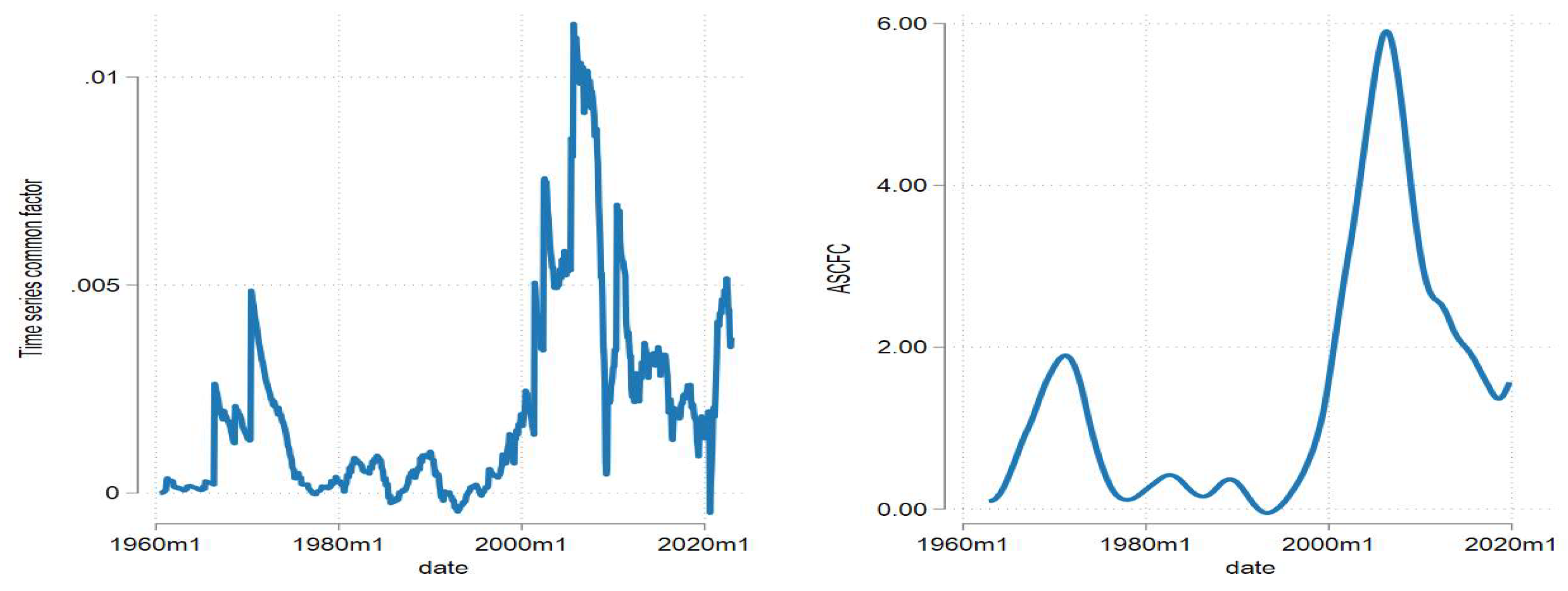
Figure 2.
Regime probabilities for entering ASCFC entering a contractionary phase; Source: Stata estimates.
Figure 2.
Regime probabilities for entering ASCFC entering a contractionary phase; Source: Stata estimates.
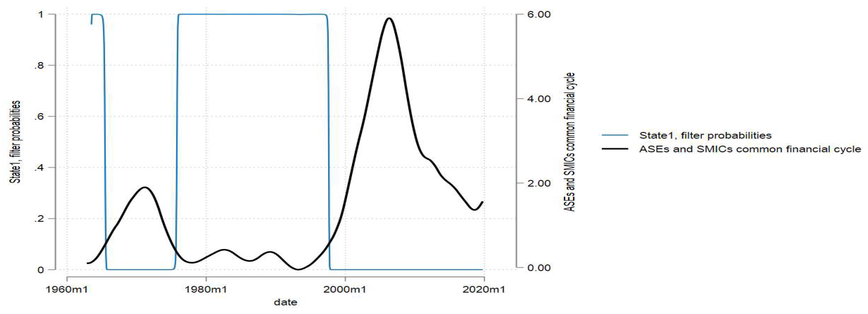
Figure 3.
Regime probabilities of the ASCFC entering an expansionary phase; Source: Stata estimates.
Figure 3.
Regime probabilities of the ASCFC entering an expansionary phase; Source: Stata estimates.
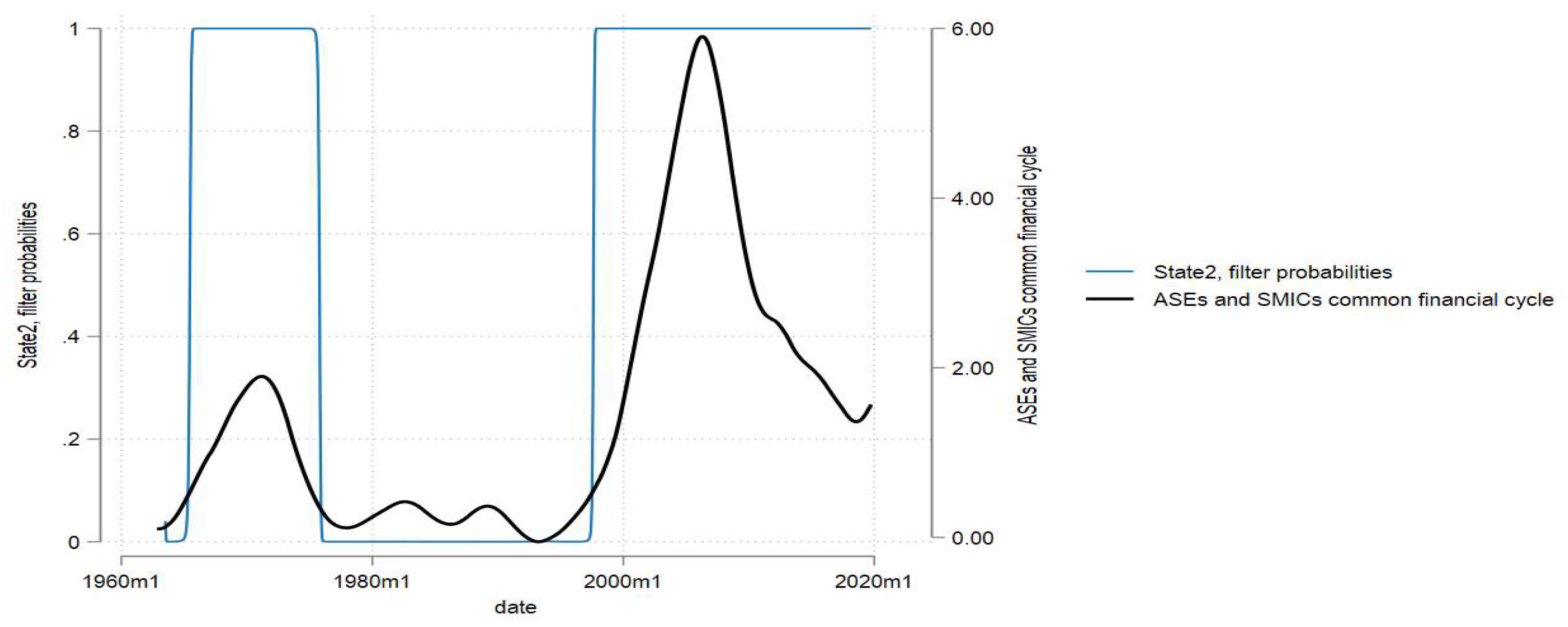
Figure 4.
The common financial cycle with different values for Source: Stata estimates.

Figure 5.
The common financial cycle with different window ranges for the BK Filter; Source: Stata Estimates.
Figure 5.
The common financial cycle with different window ranges for the BK Filter; Source: Stata Estimates.
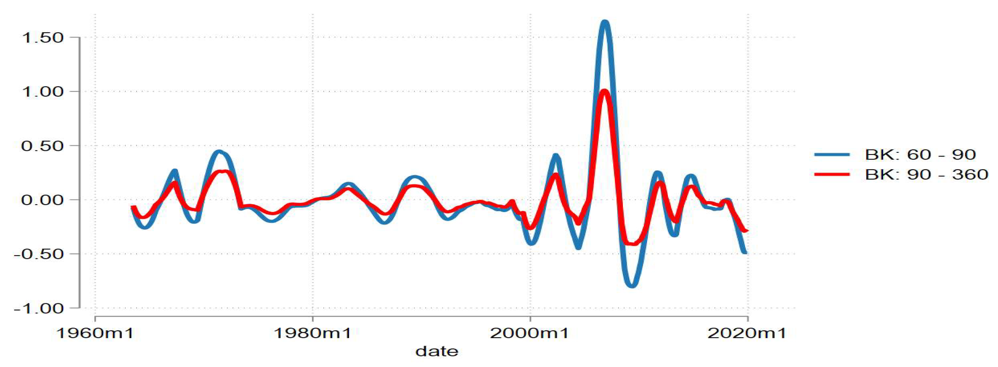
Figure 6.
Spectral density model of the common financial cycle; Source: Stata estimates.
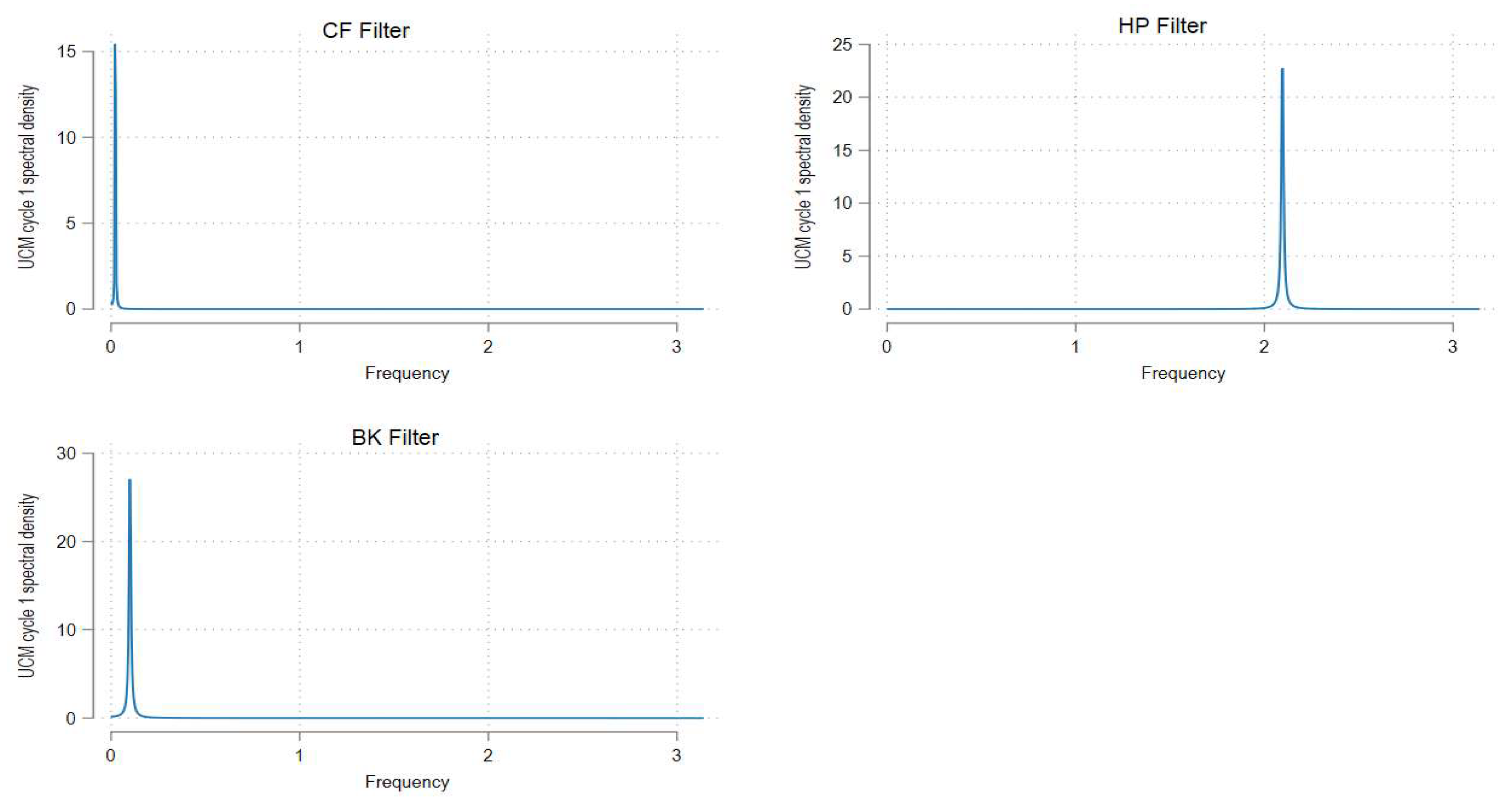

Table 1.
Data, Definitions, Sources: Common financial cycles.
| Indices | Definition | Label | Number of Variables |
| Policy rate | Official central bank policy rates | PR | 11 |
| Property prices | Real house indexes | PP | 12 |
| Share prices | Common shares of companies traded on national or foreign stock exchanges | SP | 12 |
| VIX | VIX measure of uncertainty | VIX | 1 |
| Credit | Credit from all sectors to the private non-financial sector % of GDP | CR | 12 |
| Capital flows | Balance of Payments, Financial Account, Net lending (+) / net borrowing (-) (balance from financial account), Direct investment, Net acquisition of financial assets, Equity, and investment fund shares [BPM6], US Dollar | CP | 12 |
Source: Data was collected from the Bank of International Settlements, Statistics (2023); Organisation for Economic Cooperation and Development, Macroeconomic Database (2023); International Monetary Fund, International Statistics (2023).
Table 2.
Total variance explained by common factors.
| Number | Eigenvalue | Proportion |
| F1 | 5.00 | 0.83 |
| F2 | 0.59 | 0.10 |
| F3 | 0.20 | 0.03 |
| F4 | 0.11 | 0.02 |
| F5 | 0.06 | 0.01 |
| F7 | 0.04 | 0.01 |
Source: Stata estimates.
Table 2.
Factor loadings of the common financial cycle.
| Variable | Loadings |
| ASEs and SMICs capital flows index | 0,93 |
| ASEs and SMICs credit index | 0,93 |
| ASEs and SMICs property prices index | 0,95 |
| ASEs and SMICs policy rates index | 0,88 |
| ASEs and SMICs share prices index | 0,95 |
| VIX | 0,73 |
Source: Stata estimates.
Table 3.
MSDR attributes of the common financial cycle.
| Variable | MSDR |
| c | -0,11*** |
| c | 0,03*** |
| c | 0,06** |
| c | 0,04*** |
| Transition matrix parameters | |
| P11-C | 0,75*** |
| P21-C | 0,66*** |
| Typical duration (in months) | |
| Expansion phase | 244,03 |
| Contracting phase | 210,28 |
| Overall (Years) | 37,8 |
| Transition probabilities | |
| p11 | 0,93 |
| p12 | 0,06 |
| p22 | 0,97 |
| p21 | 0,02 |
Source: Stata estimates; Notes: *, **, *** indicate statical significance at 10, 5, and 1 percent, respectively.
Table 4.
Unobserved component model of the common financial cycle.
| CF filter | HP filter | BK filter | |
| -3,85*** | -0,84*** | -4,63*** | |
| -3,59*** | -4,06** | -3,96*** | |
| 0,02*** | 2,10*** | 0,10*** | |
| 1,00*** | 0,99*** | 0,99*** | |
| 275,80 | 30,00 | 62,46 |
Source: Stata estimates; Notes: *, **, *** indicate statical significance at 10, 5, and 1 percent, respectively.
Disclaimer/Publisher’s Note: The statements, opinions and data contained in all publications are solely those of the individual author(s) and contributor(s) and not of MDPI and/or the editor(s). MDPI and/or the editor(s) disclaim responsibility for any injury to people or property resulting from any ideas, methods, instructions or products referred to in the content. |
© 2025 by the author. Licensee MDPI, Basel, Switzerland. This article is an open access article distributed under the terms and conditions of the Creative Commons Attribution (CC BY) license (https://creativecommons.org/licenses/by/4.0/).
Copyright: This open access article is published under a Creative Commons CC BY 4.0 license, which permit the free download, distribution, and reuse, provided that the author and preprint are cited in any reuse.


