
Submitted:
13 December 2024
Posted:
16 December 2024
Read the latest preprint version here
Abstract
Using a bivector model of quantum spin, and only Classical Mechanics and Special Relativity, we find the correspondence between the classical and quantum domains. Spinning to relativistic velocities reveals a symmetry break point where classical reflection becomes quantum parity.
Keywords:
quaternion spin
; dirac field
; quantum coherence
; wave-particle duality
; neutrinos
; parity
; anyons
; Twistor theory
; quantum theory
1. Introduction
Complementary pairs: energy-time; momentum-position; angular momentum-angle have classical correspondence as Planck’s constant becomes negligible. Spin is different. It is postulated as a purely quantum property of intrinsic angular momentum with no classical correspondence. In this paper, we show that correspondence exists. By using a classical model of spin, space bifurcates into the quantum domain of parity at relativistic velocities.
This work was motivated by the EPR paradox, [1,2,3,4,5,6,7], by showing the violation of Bell’s Inequalities, [8], is due to quantum coherence from a bivector. Our modified definition of spin angular momentum,
includes the geometric helicity defined by,
As a result, rather than spin polarization, , we have a unit quaternion, . Here describes the polarizing field. This formulation led to modeling Equation (1) as a classical bivector, and the results strongly supports this structure for Q-spin.
1.1. Summary
We present a detailed analysis of the geometry since the classical correspondence of spin is in its details. The main points are in the classical model, Section 3; the Discussion, Section 10; and the Conclusions, Section 11. Everything presented is also expressed and justified by Quantum Filed Theory, [2]. This means that the classical model gives way to quantum mechanics at a break point. The main parameter is the angle , between a spinning vector and its cone of angular momentum that results from the spinning.
Here is a summary of our proceedure.
- Please see the video with a brief introduction, [1].
- We create a classical model of a vector and a bivector, Figure 1 top
- Parity Symmetry Breaking: As the cones enlarge, they meet at their reflection plane, Figure 5, inset, and the reflection is bifurcated into forward and back reflections as the mirror plane shatters into left and right coordinate frames.
- The steps from zero precession up to relativistic velocities are given is Section 6
- The system moves into the quantum domain and the classical bivector model shows the growth of a resonant boson spin of 1, with no physical axis. With increased precession, the system ends with the original vectors interchanged with their bivectors, Figure 4, bottom.
- Nature uses a polarizing field to determine outcomes of , spin is Nature’s qubit.
- See a flow diagram of the quantum process, Figure 6 which follows the classical evolution.
2. The Quaternion Description of Spin
The motivation to change the symmetry of spin angular momentum from the SU(2) to the quaternion group, ,2,3], lies in the well known expression for the geometric product of Pauli spin matrices by, [9,10,11],
The first term is the symmetric scalar product formed from the anti-commutation of the components, , and the second is expressed by the Levi-Civita anti-symmetric tensor, and the bivector, . Since i cannot simultaneously be equal and not-equal to j, this expression is complementary and the two contributions are dual. Therefore, at the most fundamental level, spin possesses the distinction between symmetric and anti-symmetric. There is, however, no bivector in the Dirac Equation, [12], and introducing one is our departure from the usual treatment by Dirac. His equation for a free flight particle is
The solutions are well known, [13], giving a matter-antimatter pair, [14], and interprets spin as a point particle in Minkowski space. The Dirac field is expressed by the gamma matrices, , and the Clifford Algebra is [10], giving one time and three spatial components.
We introduce a bivector into the Dirac equation by multiplying one of the gamma matrices by the imaginary number giving the replacement, , leading to a non-Hermitian Dirac equation,
where
The subscript s denotes spin spacetime. Note that the two spatial axes, 1 and 3, can only form a plane. Also they are indistinguishable in the isotropy of free flight. Therefore if we interchange the 1 and 3 labels with a permutation operator, , the spatial components are unchanged, but the bivector changes sign, giving two solutions, .
The permutation operator, , is the parity operator for a plane, , because it interchanges a left handed frame, LHF, between a right handed frame, RHF. Therefore, the two states, , are mirror images of each other, as shown in Figure (Figure 2). This reflection symmetry is evident in Figure (Figure 1), Top panel. Since the two bivector components are counter precessing with equal frequency, they have opposite handedness.
We live in Minkowski space, with three spatial dimensions, and we are trapped in one frame, call it RHF. We can never get to the LHF, but we can see it in a mirror reflection of it, where left and right are interchanged. In our domain, they are are mixed together. Both the matter that is used to make a machine, and the torques that make the wheels turn, are both in our domain. Coherence is a property described in the same classical convex set as matter. In contrast, in the quantum domain, left and right are separated into matter and torques.
These points are needed to interpret the non-Hermitian Dirac Equation (5). Complexification of the Dirac field, gives two solutions, one is in a RHF and the other is in a LHF, as seen from Equation (6). The two solutions are mirror images, and complex conjugates of each other, Figure (Figure 2). Moreover, the signature of Equation (5), has changed to , two times and two spatial components. The second time is the period of the helicity. The two spatial compenents form a plane.
We assert that the non-Hermiticity is required for the correct description of spin reality. It needs both polarization and coherence. To accommodate this, Nature must be complex and the two conjugates be mirror reflections. This is consistent with Twistor theory, [15,16] which complexifies Minkowski into Twistor space, T. The two helicities, , are projected onto real space when measured. We do the same here. We start with the usual four dimensional real manifold of the Dirac field, , complexify it, which we denote by, , and apply parity to get the two projective helicity states in opposite frames, . The subscript s denotes spin spacetime, [2].
3. Classical spin
Figure (Figure 1) depicts the quantum and classical structures of quaternion, or Q-spin, [2,3,4]. The Bottom panel shows the two orthogonal spin axes, 1 and 3, which are spun by the axis of linear momentum, 2, which is also the Laboratory Fixed Frame, LFF, axis so . The bisector of the 1 and 3 axes forms a mirror plane, and the presence of the bivector, , is responsible for the resonant and composite boson formed from the 1 and 3 axes, as shown in the Bottom panel of Figure (Figure 1).
We consider a classical analogue of Q-spin in the Top panel. The 1 and 3 axes are massive, and the 2 axis is massless. The system is spun by the 2 axis, which is a spinning vector, and generates internal torques on the 1 and 3 axes. These counter rotate to conserve angular momentum, creating a classical bivector. Following the quantum treatment, we express this classical geometric structure as a quaternion, with vector and bivector expressed as a field over a convex set, [17] ,
where,
Here, is the vector component associated with observable classical properties of polarization, while is the bivector component creating classical coherence. As the 2 axis spins, it generates a cone of angular momentum which forms an angle, , with its axis, Figure (Figure 3). As the precession increases, so does that angle, thereby giving a continuous distribution and transfer between vector and bivector character as the geometric sum of the two.
4. Classical Motion
As the massless 2 axis turns, it generates a disc and drives the bivector. We assume the rapid spinning approximates a continuous mass distribution, so with each axis having mass of m, we will assume the disc has moment of inertia of . There are no external torques and the system is conservative, so Euler’s equations, [18],
where L angular momentum of a rigid body, and is the internal motion from the bivector reduces to,
The three coupled equations are,
and the constant angular velocity around the 2-axis, , couples to the 1, 3 axes, which are governed by,
The solutions, as expected, are counter precessing axes with frequencies of . Conservation of angular momentum requires the bivector axes to precess with twice the frequency of the disc. We recognize that the energy from the constant vector precession of the 2 axis not only causes the disc to rotate, either left or right, but also generates the internal motion of the bivector, with rotational kinetic energies of,
indicating that the bivector can hold four times as much energy as the disc for this choice of moments of inertia. The system is driven only by the conservation of energy and angular momentum, with the torques balanced between vector precession and bivector counter-precession. Torques change angles, and not the magnitude of angular momentum, , so its length remains constant while the angle between the vector and its axis, , increases with increased . The system transfers kinetic energy between the two modes as more energy is pumped in, maintaining the 1:4 ratio, but the system is far from full. The higher the energy, the faster the system precesses, and to add more energy, the 2 axis must turn ever faster. Figure (Figure 3) shows the classical motion for the two counter-rotating bivector axes. As the precession frequency increases, the cones from the angular momentum vectors, and , expand. As they widen, the parallel components to 1 and 3, , increase along the bisector, 13, and the perpendicular components, , decrease. The two axes are completely reflected, with the plane 13, separating left and right handed coordinate frames.
A spinning bivector is analogous to a superconductor where the system responds to increase in current being pumped into a coil to produce an ever larger magnetic field. In our system, there is a smooth and continuous exchange of vector and bivector components with changing energy, and their continuous mixing can be is expressed by the single convex set, Equation (7).
Relativistic effects, discussed below, are constrained by the rim velocity of the precessing angular momentum vector, which asymptotically approaches the speed of light c. The relativistic angular frequency, , is given by,
This ensures does not exceed c, preventing infinite velocities. The divergence of reflects relativistic time dilation effects, and not a physical increase in velocity. Although approaches infinity in our rest frame, time dilation on the cone compensates by decreasing the angular velocity, . As the cones widen and the radius R increases, the angular frequency, , must decrease to satisfy the condition . Eventually, the vector cones are projected into their orthogonal planes, along with their mass and chirality: the vector components vanish; and the angular velocity approaches zero. At this point, time no longer exists. The particle that remains has its left and right entirely separated and its chirality encoded into its massive structure.
5. Parity Breaking
The bivector structure is the simplest that can accept energy and endow spin to a particle. Only microscopic particles can jump to light speed. In the process they break through their symmetry plane and Nature bifurcates.
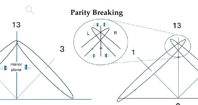
At this critical point, Figure (Figure 4), the angular momenta of the two axes meet at the reflective plane, 13. As they break through, handedness is separated from reflection. The blowup of the panel shows the symmetry breaking. Both 1 and 3 axes are still reflected, but forward and backward from the front and back of the mirror plane. Now part of the reflection is from the RHF and part is form its LHF. Chirality is separated and we can now superpose the L and R reflections to construct states of definite parity.
To express this transition from our classical domain of only reflection, to the quantum domain of distinct parity, , superpose the two reflective states, , into, [2],
with definite parity,
To form parity, both the left and right reflections, , must first be obtained. This is possible in the quantum domain, but not in ours.
6. Regions of Precession
The frequency of the precessing disc forms an angle , between an axis and its angular momentum vector:
- Classical birth: When motion begins, : the 2 axis starts to turn. The torques are too weak to couple to the bivector.
- Classical: When : At low precessional rates, the system displays only vector properties.
- Classical: When : As increases, the constructive alignment of the two angular momenta along the bisector becomes more apparent but the vector character dominates.
- Symmetry break point: Classical ⇄ Quantum at : The system reaches a purely resonant state where the angular momenta of axes 1 and 3 align perfectly along the bisector 13: the 1 axis component passes to the 23 plane; the 3 axis component passes to the 12 plane, with a combined magnitude of : a spin 1 coherent boson. This state has stability like a gyroscope.
- Quantum domain: When : The two angular momenta continue to contribute constructively to the bisector, , which now decreases in magnitude. The system remains in a counter-rotating precessional state, where vector and bivector character are separated, and quantum effects dominate.
- Quantum death: When the system is devoid of polarization, and is a pure coherent bivector state where the vectors become planes and have moved to frames of opposite handedness. Left is fully separated from right. There is no motion nor time.
7. The Resonant Boson
At the two axes of angular momenta align along the mirror plane, Figure (Figure 4), and their behaviors are influenced by relativistic effects from then on. This is a bifurcation point because the quantum domain begins and the classical domain ends. However, with increased energy the geometric composition shifts to its bivector. Indeed one can imagine that in the regime from to , the frequency, , might act like a lens by varying to favour odd over even reflection. This is an example of Maxwell’s demon.
The resonant angular momentum is formed from coherent coupling, and the two parallel components, one from 3 and the other from 1, constructively interfere forming a bivector, . The growth of this coherence is the combined contributions from the two projected rotating axes, as shown in Figure (Figure 5). The system is a coupled oscillator, where energy is exchanged between the angular momenta of axes 1 and 3. To this point, the system was effectively classical and precessed as two cones. At the two aligned vectors along the bisector give a maximum value of . This is a classical boson spin of 1.
There are now two distinct realities. From then on interactions depend on chirality: Left-handed particles interact differently from right-handed ones. Fermions can be distinguished from bosons.
At , there are equal quantities of vector and bivector components,
In order for the quaternion system to completely pass the mirror plane, it must transition to a pure bivector. As discussed above, relativistic effects flatten the cones into their orthogonal planes, lower panel in Figure (Figure 4), depicting the final relativistic limit at giving fully formed orthogonal wedge product planes with opposite chirality. The two orthogonal vectors that reflected in the classical domain have become two orthogonal bivectors that now reflect from their opposite frames. The quantum domain ends.
The quantum domain exists between and where energy and chirality work hand-in-hand to create matter. We express the two properties in the quantum domain as breaking into two convex sets,
where ⊕ is the Minkowski sum which combines elements from different convex sets. The quantum vector field with even parity is separated from the bivector field with odd parity. These give the quantum components that define Q-spin,
The angle is still relevant as it exceeds , but now the geometry includes a separated bivector, a second rank tensor, in addition to a vector, a first rank tensor. The symmetries of the two convex sets is different. The system undergoes a transition from the classical convex set, to two Quantum convex sets, for vector and bivector states. This symmetry breaking forms the complementary spaces of spin, [2,5], by separating Equation (5) into distinct equations by adding and subtracting, which separates the Hermitian part from the anti-Hermitian part,
and
This is evident from Figure (Figure 2). Adding the right and left cancels the quaternion axis 2, and subtracting cancels the two spatial terms, 1 and 3, leaving only the bivector. Our operation has separated matter from it torques. The even parity states are governed by a two dimensional Dirac equation of polarization, and the odd parity states by a massless Weyl equation of helicity. [2],
- Vector Space: Clifford Algebra, Cl(1,2), [10] (disc-like structure)
- Bivector Space: (representing quaternions and generating torques.)
Figure (Figure 6) shows the changes due to complexification, and this flow is followed by both QFT, and by Classical Mechanics with Special Relativity.
The parity separation implies that these spaces are distinct and complementary, and therefore dual,
As such, the vector component and the bivector component , cannot be observed simultaneously: they belong to different convex sets: either you are in the even parity domain, or you are in the odd. Either you are looking from a right handed frame or you are looking from a left-handed frame. The broken mirror of the parity domain separates left from right, and these must be combined into our even parity states for reflection, or into odd parity states, which would confuse us. The even parity states would reflect matter as normally. The odd parity reflection would show directional asymmetry due to forces, to which we cannot relate. In the quantum domain, the even parity of matter, Equation (20), is mediated by the odd parity of coherence, Equation (21).
8. The Bivector
This classical mixing within one convex set, Equation (7), continues as shown in Figure (Figure 5). With increased precession, the vector magnitudes, , decrease and the orthogonal components, , grow perpendicular to the axes of each cone, 1 and 3. The system is now quantum. The two angular momentum project onto their orthogonal planes of 23 and 12, which are the components , Figure (Figure 5). They constructively interfere until the angular momentum from each axis attains a cone angle of . Then both angular momenta, and , align along their mirror plane, 31. Since , there is no scalar component. However, angular momentum is transferred to the bivector by the two projected components, . The resulting bivector bisects the 13 plane. Maximum alignment occurs for and the bivector attains the value, . When the two components are maximally aligned, the increase in constructive contribution allows for more angular momentum than from the two axes separated, thereby stabilizing the bivector spin.
The bivector is the wedge product of the two angular momentum vectors from the two axes,
and represents the plane in which the two angular momenta couple. The magnitude of this bivector
reaches its maximum when the angle between the vectors is giving,
when the angular momenta are unit vectors. Due to the orthogonal geometry of 1 and 3 axes, once passes the magnitude begins to decrease.
The bivector, , lying along the bisector of 1 and 3, Figure (Figure 4), changes sign under parity exchange of the 1 and 3 axes. The bivector is odd to parity; chirality is encoded in the planes orthogonal to the 1 and 3 axes. Polarization moves into the coherent bivector.
The bivector is a boson of spin 1. The angle represents the maximum symmetric precession in the plane defined by and . This bivector, with a projection magnitude on the 1 and 3 axes, , and with a magnitude of ,19], is identified as a boson spin of 1, . It is angular momentum with no physical axis but rather pure resonance. The boson of Q-spin is virtual angular momentum and arises from our classical calculation, with no quantum assumptions..
These steps follow the system as it transitions from pure classical vector, to pure bivector beyond the quantum domain. It appears that the quantum behaviour fluctuates between and in order to balance coherent motion. This is because in that domain, energies and frequencies can engage; mass and energy are exchanged; and quantum events, from resonances in a wave environment, dominate. This is where our quantum mechanics works and classical mechanics fails. Relativity keeps systems from , and the internal frequencies, , reveals structure. Eventually, as the relativistic drags increase to the limit, the quantum nature fades, motion and time slow, and the once energetic vectors become obese, crushed and motionless. They have transitioned into a state of compression, resembling a building block of a Black Hole. Besides mass, locked within its structure, is its chirality.
9. Nature Chooses Chirality
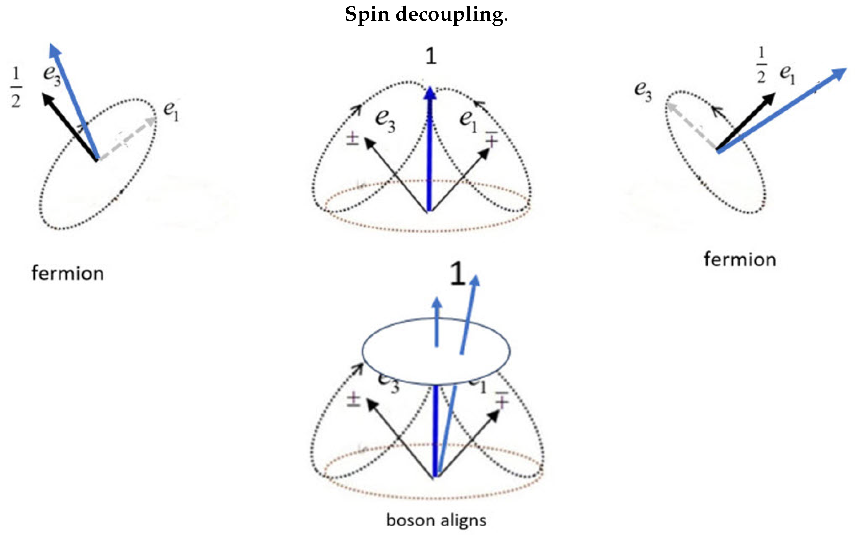
In previous publications, [2,4,5], we have displayed Figure (Figure 7). This shows the interaction of Q-spin with a polarizing field, and leads to a deterministic outcome of the polarized states of up and down.
Our mathematical treatment of Q-spin relies on the isotropy of space which allows the permutation of the 1 and 3 axes to be a parity operation. However, in free flight, the boson spin-1 is present and the anisotropy of a field causes it to align, bottom middle panel. Note that each axis has equal and opposite magnetic moments, , and the bivector has .
As the particle first approaches the field at a distance, Least Action dictates the strongest interaction will prevail. The environment is only weakly polarized. The intact bivector becomes polarized first and precesses as shown in the lower middle panel of Figure (Figure 7). As the surrounding anisotropy increases, its direction becomes more noticeable relative to the bivector precession. This will favour one side over the other. This choice is more pronounced if the anisotropic field attracts one axis and repels the other, but in either case, deterministically choosing. The bivector nutates into the direction of most attraction, which aligns, and responds like a usual fermion of spin . It has the same helicity as its chirality. Its orthogonal axis rapidly spins. What remains in the polarizing field is a fermion with definite chirality because its other hand was averaged away, left and fight panels of the figure.
We conclude that Nature’s choices are deterministic. Mistakes cannot be tolerated in the quantum domain: it is either left or right. Some processes in Nature are chiral selective, with a preponderance of one over the other. We believe the property of chirality is an immutable duality, and a random initial chiral choice would seal the future.
10. Discussion
There are no surprises when applying Special Relativity. The limiting internal motion is the rim velocity of the two bivector axes, Equation (14). For a spinning disc system with internal angular momenta and , the total relativistic energy can be expressed similarly to Einstein’s famous energy-momentum relation,
We define an effective mass that arises due to the internal angular momenta,
where I is the moment of inertia of the system. The total relativistic energy can then be written as,
where is the relativistic momentum from the spinning disc and its linear momentum.
The de Broglie wavelength is given as usual by the relation,
where h is Planck’s constant. For a massless particle, the relativistic momentum is . This expression assumes a point particle, with no internal structure. With a magnetic moment lying along the two axes, now merged into the virtual bivector boson with magnetic moment of , helical motion generates an electric field by Faraday’s Law. This leaves a trail of a helical electric field, even in the absence of charge. This field can become large as the speed increases. Thus, the electromagnetic effects associated with the rotating disc can dominate over the wave-like properties due to relativistic point particle. Therefore, includes contributions from the self-induced field,
and the de Broglie wavelength is modified to,
which includes , the contribution from the spinning and internal motions; the Boltzmann constant; and T the temperature. This effective wavelength is a measure of the particles extension, so its cube is the volume of our relativistic classical bivector system.
Using the mass of an electron and a radius defined by the de Broglie wavelength, we found for an angle of a rim velocity of m/s, or about 0.125c, is needed. It would be reduced by the EM factor, and we expect the electromagnetic effects, , to become dominant at these high velocities.
We have described how relativistic effects of length contraction, and increased moment of inertia, , compress and confine mass and energy into the planes. Energy reaches saturation when . Before this occurs, the energy resonates within the bivector structure. Classical mechanics fails (ultraviolet catastrophe), quantum effects emerge as energy sets up standing waves. The classical angular can be rewritten in terms of the de Broglie wavelength,
Substituting the wavelength for a circular orbit of radius r gives:
The initial classical bivector representation of spin serves as the geometrical and algebraic basis for the quantization of angular momentum.
This analysis demonstrates how Classical Mechanics and Special Relativity are all that are required to create the environment for Quantum Mechanics.
10.1. Continuous Complementarity
The identification of the parity symmetry breaking, defining the Classical-Quantum boundary, begs the question about the other complementary: energy-time, momentum-position, angular-momentum and angle, and if they resulted from symmetry breaking. We assert they do not. Parity breaking alone is all that is needed to distinguish our reflective domain from the microscopic symmetry where chirality is separated. Parity is Nature’s qubit, and the only property needed for logic. It must be deterministic.
Looking again at the early Universe with defined chirality, we note that time was irrelevant. Every chaotic particle with relativistic energy existed in a distinct inertial frame where time changes for every particle. Time was randomized. Only when expansion settled into collective motions whereby large inertial frames, like our domain, existed, did Time become relevant. Then Time becomes balanced with even-parity energy, giving order and structure to the Universe from which Time emerged with a definite direction as shown by Boltzmann’s H-theorem, [20], with the opposing consequence of disorder and increased entropy.
For Nature to proceed, it must distinguish odd and even, fermions and bosons. In the early Universe all microscopic particles would respond to chirality: the only and first symmetry in that chaotic nascent period. The only mechanics was quantum mechanics.
Likewise in those early Epochs, position and angle were also of little relevance, since they changed so rapidly. Only the wave properties of momentum and angular momentum were relevant. Moreover, the motions of waves are related by boosts and rotations between inertial frames. Neither commute, indicating that non-commutation was an essential property of early Universe, and remains so today for quantum systems. It is also clear that these properties are inverses of their complements, with energy, momentum and angular momentum requiring, inverse mathematical representations for time, position and angle, at least in the quantum domain. These inverse properties lead to the Heisenberg Relations and natural dispersion. Their continuous symmetries are consistent with Noether’s Theorem, [21], whereby the invariance of the action is conserved. This type of complementarity is entirely different from parity, which is a discrete symmetry with binary outcomes.
Within the non-Hermitian Dirac equation, there are two times. Linear time, associated with linear momentum remains in even parity space, whereas the second time is the period of helicity, and can evolve into the future, or the past, with equal ease, underscoring that Time conjugation operator involves complex conjugation: it flips between the two projective spaces of the complex Dirac field, , thereby defining Time as opposite in the two helicities spaces.
11. Conclusions
From our bivector model, an intuitive geometrical framework for understanding angular momentum is obtained. A spin- need not be postulated but develops from a classical vector to a quantum bivector. Energy and angular momentum are conserved over both domains giving continuity between classical and quantum mechanics. From low frequency birth as a classical spinning vector, to its relativistic demise as a bivector, the two orthogonal planes become locked into handedness of a massive spec in the cosmos.
Parity separation starts at , when the bivector undergoes a bifurcation. Handedness has a classical origin showing parity differs between a vector and bivector,
As a classical bivector becomes a quantum Q-spin, Equation (1) is justified. Classical notions of angular momentum connect with quantum helicity, chirality, coherence and entanglement. Quantum spin emerges from underlying geometrical and relativistic structures of the classical domain. Information and structure of Nature appears based upon her ability to treat the handedness as a natural qubit. Learning how to control the handedness of an electron might benefit quantum computing, avoiding unstable qubits and decoherence.
We assert that the dynamic origin of Q-spin means the property of parity is immutable, along with the immutability of T and C symmetries. These fundamental discrete conservation laws are based on the geometry of space-time rather than the forces of Nature. We suggest that a particle should include in its definition, the adherence to the individual symmetries of P and C and T. This implies that neutrinos do not exist, and the suggestion seems to fly in the face of the famous Wu experiment in 1956, [22]. However, Q-spin is a boson of odd parity, meaning that beta electrons are odd to parity. This reveals that under the quaternion symmetry, parity is not violated, and neutrinos are not needed, [7]. This does not mean the Wu data is incorrect, only re-interpreted.
Quantum phenomena as described by current quantum mechanics are probabilistic, indicating Nature is fundamentally statistical. Q-spin shows that Nature is deterministic. She uses the even parity of energy to create the structures of the Universe, and the odd parity of bosons to mediate the processes. This distinction fails at the peril of evolution, suggesting once again that parity is immutable, and Nature’s choice deterministic.
Parity of photons and gluons is odd. If the Weak force symmetry, SU(2), is replaced by the quaternion group, , then Q-spins should replace the Weak gauge bosons (), none of which are eigenstates of parity. We believe that all bosons are odd to parity, otherwise Nature’s parity choices are not consistent.
The question arises if the final massive gyroscopic spec could be the origin of a Black Hole as the termination of the spinning quantum structure transitions entirely into a relativistic mass concentration. It shares properties with a Black Hole, for example, the transition from quantum to its demise occurs as the system’s internal degrees of freedom become locked. Our spec resemble the behavior of matter near the event horizon of a black hole, where dynamics appear frozen. It could lead to curvature of space-time, similar to the properties of a black hole, with interesting spacetime dynamics if the structure is two orthogonal planes, rather than a point.
The classical correspondence of spin confirms symmetries and geometries of the classical domain carry over to the quantum domain. Parity separation reveals harmony and balance between the quantum and classical. They are tied by conservation laws, and unified by symmetry, geometry, and dynamics. Nature bridges these domains where determinism is essential, and ontology complex.
References
- Video: The classical origin of spin, https://youtu.be/LpneCCyK5Js?
- Sanctuary, Bryan. Quaternion Spin. Mathematics 2024, 12, 1962. [CrossRef]
- Sanctuary, Bryan. Spin Helicity and the Disproof of Bell’s Theorem. Quantum Rep. 2024, 6, 436–441.
- Sanctuary, Bryan, Non-local EPR Correlations using Quaternion Spin. Quantum Rep. 2024, 6(3), 409–425. [CrossRef]
- Sanctuary, Bryan, "Quaternion spin: structure and properties, Submitted, 2025.
- Sanctuary, Bryan, "Bell’s theorem", 2025.
- Sanctuary, Bryan, "Quaternion spin: parity and beta decay", 2025.
- Bell, John S. "On the Einstein Podolsky Rosen paradox." Physics Physique Fizika 1.3 (1964): 195.
- Doran, C. , Lasenby, J., (2003). Geometric algebra for physicists. Cambridge University Press.
- Hestenes, D. , and Sobczyk, G. (2012). Clifford algebra to geometric calculus: a unified language for mathematics and physics (Vol. 5). Springer Science and Business Media.
- Wikipedia contributors. (2024, ). Pauli matrices. In Wikipedia, The Free Encyclopedia. Retrieved 12, 12 July 2024; :06.
- Dirac, P. A. M. (1928). The quantum theory of the electron. Proceedings of the Royal Society of London. Series A, Containing Papers of a Mathematical and Physical Character, 117(778), 610-624.
- Peskin, M.; Schroeder, D.V. An Introduction To Quantum Field Theory; Frontiers in Physics: Boulder, CO, USA, 1995. [Google Scholar]
- Dirac, P. A. M. (1930). "A Theory of Electrons and Protons". Proc. R. Soc. Lond. A. 126 (801): 360–365.
- Penrose, Roger. "Twistor algebra." Journal of Mathematical Physics 8.2 (1967): 345-366.
- Penrose, Roger. "Solutions of the Zero-Rest-Mass Equations." Journal of Mathematical Physics 10.1 (1969): 38-39.
- Morris, C. C. , and Stark, R. M. (2015). Finite mathematics: models and applications. John Wiley and Sons.
- Goldstein, Herbert, "Classical Mechanics", Addison Wesley Publishing Company, 1980.
- Sanctuary, B. C. (2007). The two dimensional spin and its resonance fringe. arXiv:0707.1763.
- Boltzmann, L. (1872). Weitere studien über das wärmegleichgewicht unter gasmolekülen (Vol. 166). Aus der kk Hot-und Staatsdruckerei. English translation: Boltzmann, L. (2003). "Further Studies on the Thermal Equilibrium of Gas Molecules". The Kinetic Theory of Gases. History of Modern Physical Sciences. Vol. 1. pp. 262–349.
- Emmy Noether. Invariante Variationsprobleme. Gott. Nachr., pages 235–257, 1918.
- Wu, C. S. , Ambler, E. P. ( 105(4), 1413.
- Bell, J. S. (1987). "Speakable and unspeakable in quantum mechanics" Cambridge University Press. New York, Bell’s quote is on page 65.
Figure 1.
Two properties of spin: Top: A classical model for Q-spin with two orthogonal massive axes, 1 and 3, spun around the massless 2 axis with frequencies up to the relativistic limit, . The spinning disc couples to the two axes which counter rotate to conserve energy and angular momentum. We use the classical model to show the correspondence between classical and quantum domains. Bottom: two orthogonal spin- polarization vectors, and , perpendicular to the direction of linear momentum, Y. The helicity is in the direction of propagation, , and spins right or left. The two spin- vectors, and , couple to give a composite boson, , of magnitude 1.
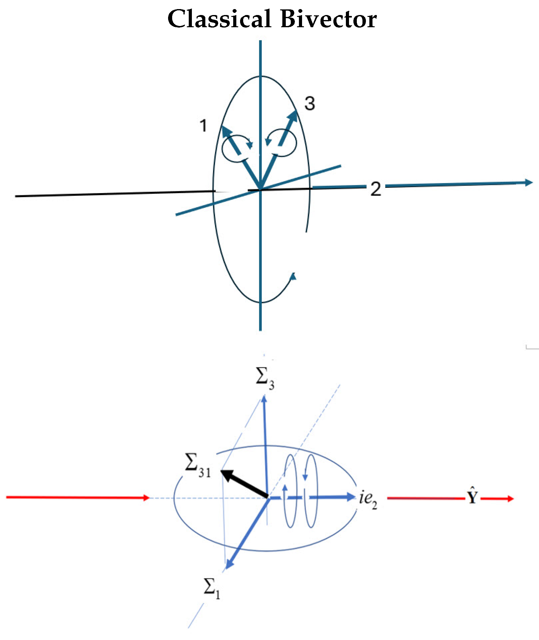
Figure 2.
The mirror states of a Q-spin with on the right and on the left. Note that adding these states is independent of and subtracting them is independent of and .
Figure 2.
The mirror states of a Q-spin with on the right and on the left. Note that adding these states is independent of and subtracting them is independent of and .
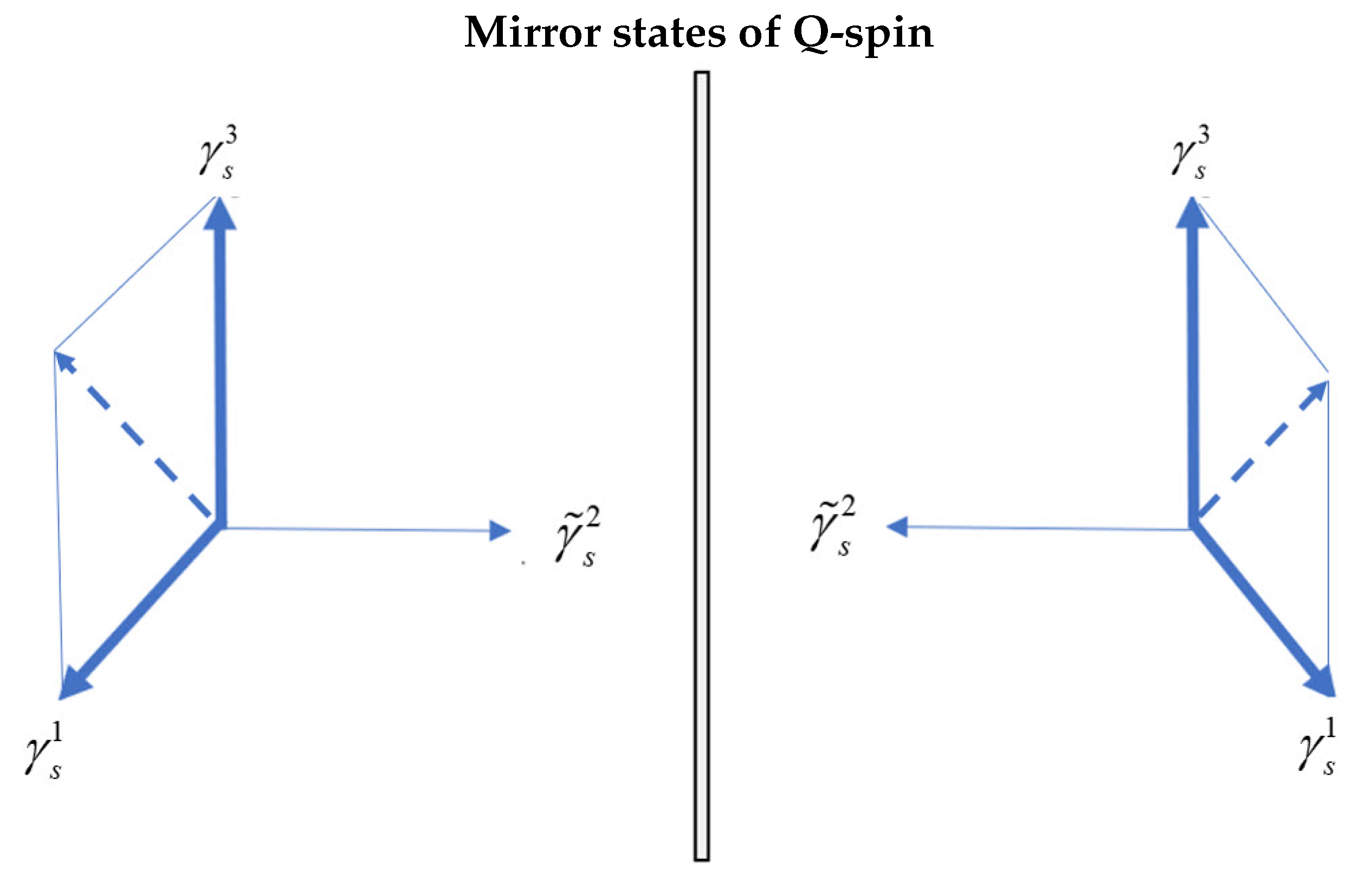
Figure 3.
The Classical domain: In the rotating frame of the disc. Showing the left and right hands of Nature. The angle, , between the axes, 1 and 3, and their angular momentum cones increases as the precession frequency increases. A mirror plane bisects the 1 and 3 axes.
Figure 3.
The Classical domain: In the rotating frame of the disc. Showing the left and right hands of Nature. The angle, , between the axes, 1 and 3, and their angular momentum cones increases as the precession frequency increases. A mirror plane bisects the 1 and 3 axes.
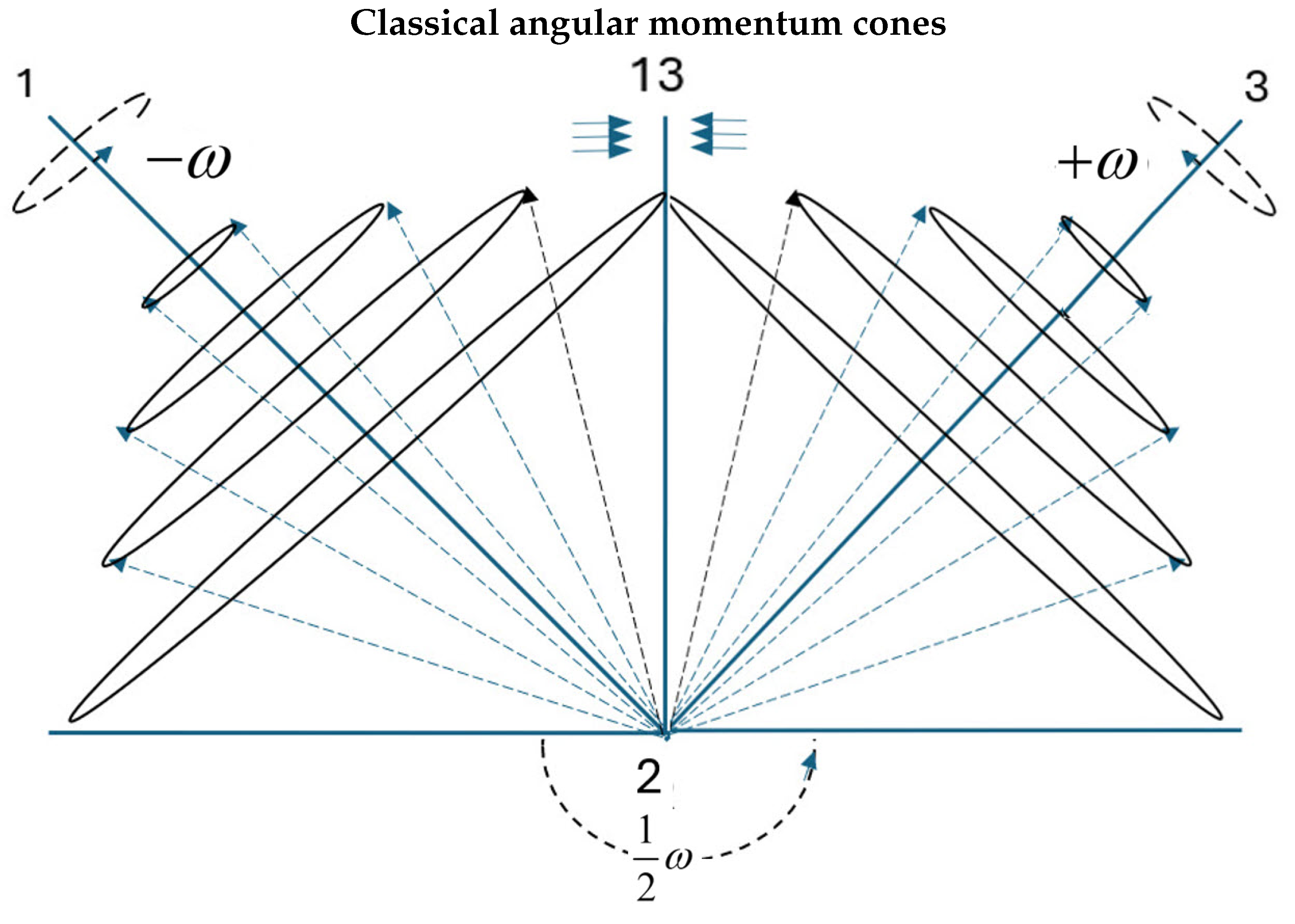
Figure 4.
The quantum domain: The top left panel shows the bivector model at the parity break point. The next panel shows left and right hands are separated into domains of distinct parity. Bottom panel. The relativistic demise with the vector motion being compressed into their opposite planes. Spin has a left and a right hand, which is the likely the reason we do too.
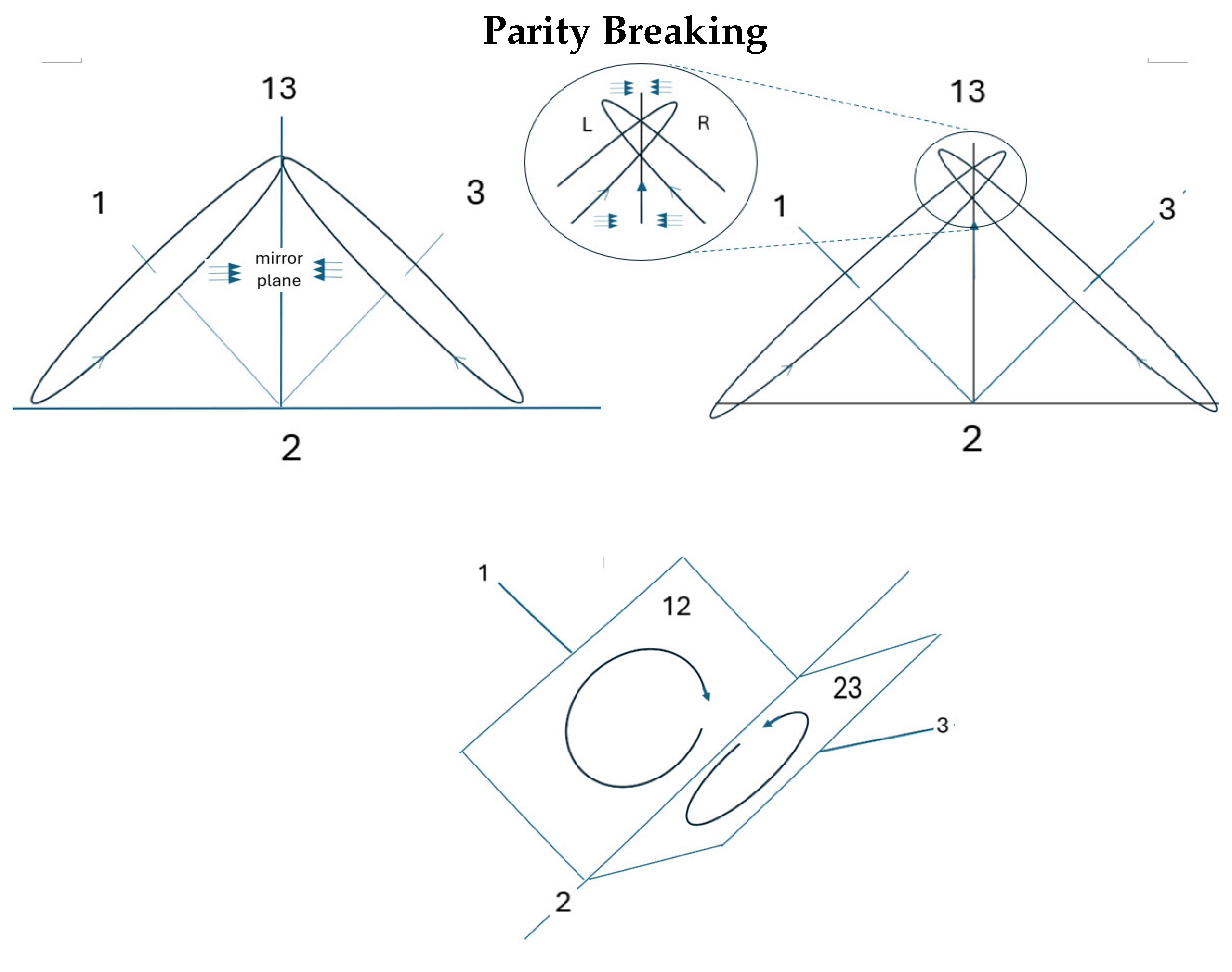
Figure 5.
The cone to the left has the angular momentum vector, , decomposed into its parallel,, and perpendicular components, . The 1 axis projects its component onto the 23 plane and the 3 axis projects onto the 12 plane. The two components align along the 13 bisector to produce a resonant bivector. Its magnitude is , consistent with the magnitude of a spin 1 boson, .
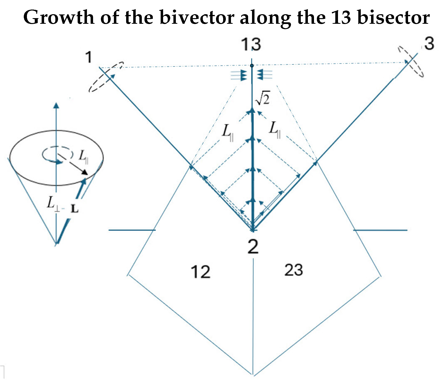
Figure 6.
The structure and separation of spin spacetime into complementary spaces of polarization and coherent helicity.
Figure 6.
The structure and separation of spin spacetime into complementary spaces of polarization and coherent helicity.
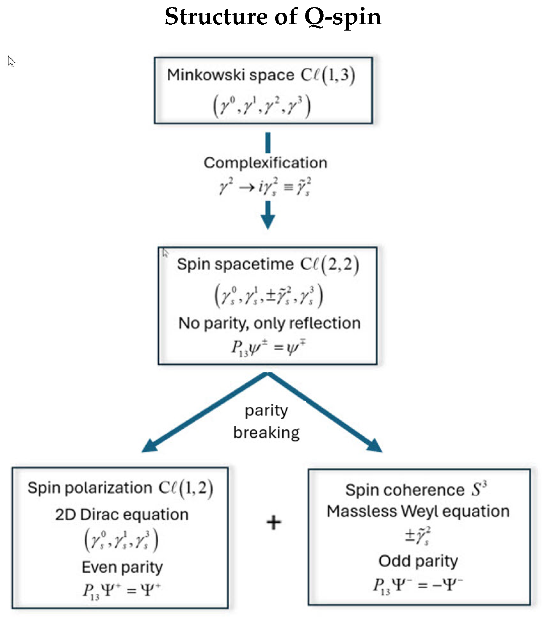
Figure 7.
The longer arrow denotes the direction of the polarizing field. Top: The two mirror states in free flight, and , couple to give a boson spin-1. Left and right: The fermionic axis closer to the field axis aligns, and the boson decouples. These two panels do not indicate two particles but one Q-spin depicted with one for the other axis aligned with the field. Bottom: When the boson spin is close to the field, it initially precesses as a spin-1 without decoupling.
Disclaimer/Publisher’s Note: The statements, opinions and data contained in all publications are solely those of the individual author(s) and contributor(s) and not of MDPI and/or the editor(s). MDPI and/or the editor(s) disclaim responsibility for any injury to people or property resulting from any ideas, methods, instructions or products referred to in the content. |
© 2024 by the authors. Licensee MDPI, Basel, Switzerland. This article is an open access article distributed under the terms and conditions of the Creative Commons Attribution (CC BY) license (http://creativecommons.org/licenses/by/4.0/).
Copyright: This open access article is published under a Creative Commons CC BY 4.0 license, which permit the free download, distribution, and reuse, provided that the author and preprint are cited in any reuse.


