
Submitted:
25 July 2025
Posted:
28 July 2025
You are already at the latest version
Abstract
There are two ways of linearizing the Klein-Gordan equation: Dirac's choice, which introduces a matter–antimatter pair, and a second approach using a bivector, which Dirac did not consider. In this paper, we show that a bivector provides the classical origin of quantum spin. At high precessional frequencies, a symmetry transformation occurs in which classical reflection becomes quantum parity. We identify a classical spin-1 boson and demonstrate how bosons deliver energy, matter, and torque to a surface. The correspondence between classical and quantum domains allows spin to be identified as a quantum bivector, $i\sigma$, which is a spinning plane. Using geometric algebra, we show that a classical boson has two blades, corresponding to magnetic quantum number states $m=\pm 1$. We conclude that fermions are the blades of bosons, thereby unifying both into a single particle theory. We compare and contrast the Standard Model which uses chiral vectors as fundamental, with the Bivector Standard Model which uses bivectors, with two hands, as fundamental.
Keywords:
classical spin
; intrinsic angular momentum
; geometric algebra
; Dirac field
; classical correspondence
; coherence
; bosons
; fermions
; parity
; reflection
; Twistor theory
; quantum theory
; standard model
; Bivector standard model
1. Introduction
When Dirac linearized the Klein–Gordan (KG) equation [1], his anticommuting gamma matrices
led to the familiar Dirac equation [2] in Minkowski space, which is the Laboratory Fixed Frame (LFF), defined by . However, an alternative linearization exists that Dirac did not know about [3,4,5]. Instead of Dirac’s choice of gamma matrices, the set
also anti-commute where
introduces a bivector [6]. The subscript s denotes spin spacetime in the Boby Fixed Frame (BFF), . Dirac’s linearization led to the identification of two spin- particles with opposite properties, establishing the matter–antimatter pair, [7]. The main issue is the negative energy of the antimatter particle which has never been satisfactorily resolved, [8]. The matter-antimatter interpretation is universally accepted. It identifies the two particles as fundamental fermions of spin . This choice leads directly to the Standard Model, [9], SM, of particles.
We have shown, [3], that the bivector linearization gives a different interpretation which resolves the negative energy issue, the baryogenesis problem, and the EPR paradox, [4,5]. The main purpose of this paper is to contrast the bivector linearization from Dirac’s choice. We argue that the bivector approach offers an alternative with consequences that may well lead to abandoning the current paradigm based upon chiral fermionic fields of the SM. Rather a Bivector Standard Model, BiSM, is suggested. In this paper we describe the electron as a physical object with a bivector structure which replaces the usual point particle of the SM.
Figure 1 compares the SM matter-antimatter pair with the BiSM bivector. Both are mirror images and both have opposite chirality. Dirac proposed two particles, and the bivector model proposes two axes on the same particle.
One of the consequences of the bivector spin is we show for the first time that intrinsic angular momentum has a classical origin. This opens up an entirely different description of the microscopic and gives insight into the fundamental properties of the quantum domain. The description of spin changes from a chiral point particle of intrinsic angular momentum, to a well defined ontic structure: a rotating plane that spans the classical and quantum domains, [3].
The consensus is, however, that spin is an intrinsic quantum property without a classical origin. No classical theory has revealed full quantum behaviour, [10,11,12,13,14,15]. These approaches universally start with spin as the fermions experimentally observed and use Dirac’s matter-antimatter choice.
Hestenes pioneered the use of Geometric Algebra, GA, to reinterpret the Dirac equation by expressing spinors as real multivectors and identifying the internal structure of spin with zitterbewegung (zbw:trembling motion) [16]. This is a rapid, lightlike circulatory motion of the electron at the Compton scale. Spin then emerges from the intrinsic rotation of a localized point-like particle, modeled as a rotor in spacetime algebra, with the complex phase of the spinor reinterpreted as a physical geometric rotation. Both Hestenes’s treatment and ours have many features in common. We find internal motion of the electron that likely is the source of a zbw. His interpretation provides a kinetic origin for the rest mass and associates the quantum phase with real rotational geometry. However, Hestenes retains the structure of Dirac spinors and relies on the conventional spinor decomposition into electron and positron states. In contrast, the BiSM dispenses entirely with spinors, modeling spin as a classical bivector confined in the BFF, with spin- projections emerging from rotor dynamics of a spin-1 structure. This difference in our approaches eliminates the need for chiral decomposition, complex amplitudes, and positive/negative energy conflict between the electon/positron pair. Rather, these are replaced with real geometric precession and internal blade coherence. Since both approaches use GA, both are focused on geometry.
Building on Hestenes’ framework, Doran and Lasenby, [6], further developed geometric algebra as a foundation for quantum mechanics and quantum field theory. Their formalism expresses spin states as even-grade multivectors, or rotors, acting on reference vectors, providing a geometric visualization of spin and spacetime dynamics. However, their approach again remains structurally aligned with quantum theory, retaining spinors as fundamental entities. They preserve complex phase, maintain linear superposition, and rely on operator algebra for measurement.
The zitterbewegung appears consistent with a structured bivector with rotating blades within a BFF. Rather than postulating internal motion from the LFF, the bivector-based model gives internal angular momentum geometry, with classical rotor dynamics governing spin, mass, and chirality. This provides a concrete mechanical origin for spin and parity, free from abstract spinor components and compatible with classical rotational motion under Lorentz conditions.
Muralidhar, [17], used GA to study the electron at zero point energy. He too finds spin is a bivector governed by classical rotor dynamics.
1.1. Outline
In Part I we present the classical mechanics of a bivector and show that its properties correspond to those of quantum spin. We identify a significant bifurcation where classical spinning separates the environment which forms spin states with definite odd and even parity. This transition reflects the change in symmetry from classical reflection to quantum parity.
In Part II we describe the symmetry transition between classical and quantum domains, and show the correspondence between classical and quantum bivectors.
In Part III we interpret the results, and describe mechanisms by which external spin chirality relates deterministically to internal chirality, enabling structure formation.
In Part IV we show the unification of bosons and fermions. Properties of internal mass-energy balance, helicity, chirality, emergence of charge are also discussed.
In Part V the ontological differences between the SM and the BiSM are discussed. We formulate the bivector field as spin 0, 1, and 2 structures. Each is related to a bivector property which leads to a Lagrangian for both the classical and quantum bivectors.
Part VI shows that superposition of bivectors does not happen, and discusses quantization and measurement.
Part VII discusses the experimental evidence that support both the SM and the BiSM.
2. Classical Spin
The results of this section establish that a classical bivector defines a classical spin-1 boson using no quantum postulates. There is a direct correspondence between classical and quantum spin. This correspondence is taken as strong support that spin is a bivector with two opposite chiral hands.
2.1. A Classical Bivector
Figure 2 shows three different views of spin. On the left is the usual point particle with intrinsic angular momentum, treated as a chiral fermion. On the right is a classical bivector in its BFF with two internal axes (1 and 3), spinning about the 2-axis of linear momentum. In the center is that same bivector but now viewed from the LFF. It is a spinning disc with the internal motion mostly averaged out. The torque, or force, around the 2 axis is in the LFF. In the BFF, that torque becomes the centrifugal force, acting along the bisector of the 1–3 axes, causing them to counter precess. This is internal motion. We also assume that microscopic particles require so little energy compared to its availability that they quickly attain a state of quantum parity by spinning the bivector to high, but not relativistic, frequencies.
2.2. Complementarity
This leads us to the first property shared by classical and quantum bivectors: complementarity. In the LFF, the observer sees a vector precessing around the 2-axis, but no internal bivector motion. We see only a projected blur of the internal dynamics, like looking at an engine when lifting the hood. From the BFF, the vector motion around the 2 axis is canceled, but there the internal torques are absorbed, driving the internal bivector dynamics, like the wheels of the engine responding to the applied torque. In the classical domain, there are two complementary views of spin: vector motion around the axis in the LFF, and a coherent bivector motion, , in the BFF, [3].
2.3. Euler’s Equations
The bivector structure shown in the left panel of Figure 3 depicts a bivector with external vector precession. The two massive orthogonal axes of the bivector are labeled 1 and 3. In response to the vector motion around the massless axis 2, these two axes counter-precess with opposite angular velocities, . Take the moment of inertia for the external vector as , and that for the internal bivector as . The bivector axes counter precess at twice the frequency of the torque axis, 2, and therefore the rotational energies, , for the disc and the two axes, are distributed between the vector and bivector in the ratio,
a ratio maintained for any precessional frequency of a rigid bivector.
The classical motion is described by Euler’s equations. The massless 2 axis provides the torque that turns the bivector either clockwise or counter-clockwise. They are the classical particle’s two helicity states. We calculate the motion at fixed frequencies so there are no external torques and the system is conservative. Euler’s equations reduce to the substantive derivative, [18],
This describes the internal motion by its angular momentum, , and the constant angular velocity around the 2-axis, giving two equations for the 1 and 3 motions,
where . The solutions apply conservation of energy and initial equal phases. Two cones of angular momentum are generated one for each axis. Their interaction plane, 13, is where the two cones are closest and furthest in their orbits, giving,
These are shown at various angles , defined as that between an axis, and the vector, , Figure 3). The units are radians per second, and G is a gauge to be determined by the system. The period of precessions is . These components are normalized: parallel to the axes is ; and perpendicular to the axis is , Figure 3).
2.4. Resonance
This configuration can also be expressed in terms of the angle between the two angular momentum vectors, and by
giving,
where the bisector axes are defined as,
With constant, the two orbits resonate between alignment along the bisector, and cancellation along opposite directions of . Therefore, the tandem and coherent precessional motion results in the two vectors at various fixed values of coming in and out of phase coherence, Figure 3). The mirror plane bisecting the 13 axes reflects them, so neither can distinguish its real counterpart from its own reflection. This figure is shown from to , or equivalently from from to 0.
From the BFF, Figure 2), the high precessional motion about the 2-axis is canceled, revealing the internal counter-precession of the bivector. The external vector precession and the internal bivector motions are related: for every period of rotation around the 2 axis, the bivector axes counter-rotate by two periods. This is a geometrical example of the double cover of SU(2) over SO(3). The angle remains fixed at constant precession. This resonance within the bivector structure is identified below as a spin 1 boson.
2.5. Geometric Algebra: Bivector Dynamics
A blade is defined as one of the two orthogonal vector axes and that are used to define spin, Equation (11) below. Chirality refers to the handedness of this bivector plane, which is determined by left- and right-handed unit quaternions around the 2, or torque, axis, [3]. In contrast to the SM, where chirality is projected from the Dirac field using , [1], here it arises from the opposite chirality of the two blades. These blades are identified as the magnetic numbers of spin, both classical and quantum.
The counter precessing cones of angular momentum, Figure 3), lead to the definition of classical spin as a bivector being the wedge product of the two angular momenta associated with each axis, [6],
thereby defining their interaction plane, 13. Using Equation (7), the scalar and the wedge products are,
Normalized gives a unit quaternion structure of a scalar and bivector which we express as the geometric product, [6], of the two angular momenta,
Spin is a bivector, Equation (11), and the geometric product, Equation (13), describes its dynamics as a classical rotor.
The unit vector is normal to the 31 plane and gives rotation around the 2 axis which is manifest in the LFF as a spinning disc. There is no vector component in the BFF. This quaternion also gives a measure of scalar and bivector contributions at different angles. The scalar part gives a measure of its mass, and the bivector part gives coherent rotational kinetic energy from the two counter precessing axes. At , the scalar part is maximized to 1, and the two axes 1, 3, meld which cancels their precessions, leaving scalar mass. Equation (4) shows that the ratio of the rotational kinetic energies is fixed. As the internal frequency goes to zero, so the external precession slows and stops. In isotropy, all kinetic energy is converted to mass. This locked kinetic energy can be revived in the presence of a polarizing field, causing the two blades to unfurl. This suggests that in isotropy and far from any target, the bivector electron conserves energy by converting it all to mass. It maintains its bivector 2D frame giving spin finite size. We call the BFF the rest frame, and the mass the rest mass. We identify this maximally confined structure to have the classical electron radius .
This classical angular momentum has no physical axis and is a purely resonant state: the eye of a tornado along 13. The analogy is apt but with an extra twist. The eye of a vector tornado is a region of calm and lower energy, yet surrounded by a vortex of high precessional energy. In contrast, the bivector tornado is due the two axes melding into an eye of left and right chiralities intertwined in harmony, Figure 3). There is no vortex, only a scalar directed along the bisector with calm everywhere else. It is a microscopic double helix. As all internal motion ceases. With no magnetic field present, we assign this state the magnetic classical (not yet quantum) number . The two blades, , have folded into a massive arrow. The high rotational kinetic energy of those two locked blades is reversibly converted into mass with changing . The chirality and energy are not lost, only stored in free-flight by the geometric product. Figure 3) also shows how the massive double helix destroys reflection, leading to parity. Shown is the even parity state of matter.
The quaternion, , is also a phase which changes sign when 1 and 3 labels are swapped. This symmetry operation shows the 1 and 3 labels are indistinguishable, allowing for both the clockwise and counter clockwise helicity around the 2 axis.
2.6. A Classical Boson of spin-1
This resonant and scalar state is formed from the coherent coupling of the two perpendicular components, , one from axis-3 and one from axis-1. As seen from Figure 3), the component from axis-1, , projects onto the 23 plane, while the axis-3 component projects onto the 12 plane. Any cone will give a spin-1, but the maximum value occurs when at . We normalize these cone projections and the angle between the projected component and the bisector, 31, is . A spin is formed from these two components which resonates giving a state of length . Using the quantum definition for the angle, , between a spin axis and its cone, we get
which is identified as a purely classical spin 1. Moreover, this particle is rapidly spinning, averaging out all anisotropies, and obeying Bose-Einstein statistics. We are justified in calling the classical spin a boson. Since the spin-1 is a result of the coupling of the two blades, we assign a spin of to , and .
2.7. Special Relativity
Using the angular momentum of an electron, , its mass, and a radius defined by the de Broglie wavelength in atomic systems of m, we found a rim velocity of m/s, or about 0.03c, is attained. This allows us to determine the gauge, G, for an electron. At let ,
Relativistic effects, [19], are determined by the relativistic angular frequency, , which is given by,
where is the Lorentz factor. The divergence of reflects relativistic time dilation effects, not an actual physical increase in the intrinsic angular velocity . At higher precessional frequencies, to compensate for time dilation, the observed precessional frequency decreases. The condition must be satisfied. As and , the system ceases to spin, and energy is converted to mass. Here is the effective coherence length or wavelength associated with the relativistic angular frequency. However, this usual explanation of the relativistic limit can never be approached by an electron because the quantum domain occurs first.
2.7.1. The Quantum and Relativistic Limits
Due to the intertwining of the two chiralities, the cones cannot pass through one another, and instead become confined as mass. The quantum limit, therefore, occurs at . At this limit, the energy is,
with and,
where is the internal rest mass. At , the electron is far from its relativistic limit. At this point, however, all rotational kinetic energy is fully confined. The double helix in Figure 3), shows the mass formed from intertwined blades, when left and right merge into a state of positive parity. This is the quantum domain. It exists only at . The intertwining of the two chiralities means the addition of more internal energy is not possible. Once the system reaches this quantum limit, additional energy cannot further increase the rest mass. Instead, additional energy propels the entire structure through space, shifting the dynamics from internal confinement in the BFF, to external forward propagation in the LFF. The relativistic limit, can never be approached internally, thereby capping the rest mass.
This establishes a geometric origin and physical mechanism for the quantum and relativistic limits. The Lorentz factor becomes a geometric measure of the quantum limit, and differs for types of particles. In contrast to the SM, which treats mass as intrinsic and structureless, the BiSM shows that rest mass arises from a structured, geometric state formed at the quantum boundary.
3. Correspondence
In this part, we formalize the correspondence showing how classical spin maps to quantum operators, and how parity bifurcation emerges geometrically. Planck’s constant is identified from the structure.
3.1. Parity from Reflection
The symmetry of our domain, the LFF, is different from the bivector symmetry of the BFF. This transition at , defines when reflection becomes parity. To see this significant symmetry transition, note our RHF domain has three spatial dimensions of definite chirality. We can never get to the LHF and see only a mirror reflection of our RHF. The matter that is used to make a machine, and the torques that make the wheels turn, are both in our RHF domain. The bivector, in contrast, has one axis in a LHF, and the other in the opposite RHF. They are mirror or reflective states, , in opposite handed frames, Figure 3). They form a chiral pair, a left and right hand of Nature. In complete contrast to us, the bivector does not see its reflection in the mirror plane, but its real opposite chiral hand.
Reflection evolves to positive parity at , when the two angular momenta lock into a double helix of mass inside their reflection plane. Reflection is lost, as shown in Figure 3), lower right. Up until the double helix of mass is formed, the left and right frames are separate and reflection preserved, but as shown, left and right reflections intertwine along the bisector which defines the quantum domain. Therefore that figure shows that the two reflections add, and they can also be substracted,
Since the system is a two dimensional plane, 31, a permutation operator, , interchanges left handed planes and right handed planes, so giving,
Therefore, a LHF and a RHF, shown in the bottom panel of Figure 3), combine into states of definite parity with the permutation, , being the parity operator,
Adding gives even parity and cancels the torque axis 2; subtracting gives odd parity and cancels the massive axes, 1 and 3, thereby separating matter from force. Thus, the emergence of quantum parity from classical reflection is a necessary consequence of the bivector structure.
3.2. Classical-Quantum Correspondence
The classical domain is described by a continuous mixture of vector and bivector motion, forming a single classical convex set. As the angle decreases, the symmetry shifts from classical reflection to quantum parity. As , the classical system transitions to two distinct convex sets, each with definite parity. This marks the bifurcation point where classical dynamics becomes quantum. In this process, force separates from matter, the former in the LFF, and the latter in the BFF. Their classical complementary becomes quantum. In this transition, the classical bivector remains intact as a bivector. It is not the bivector that changes, but the symmetry of the environment inside the BFF that causes a phase transition from energy to mass.
As the angle varies, vector and bivector motion are geometrically mixed forming a field over a classical convex set, [20],
where,
To be clear: the vector motion about the 2 axis is expressed by in the LFF, and the complementary internal bivector motion is expressed by in the BFF.
As varies, the system undergoes a continuous transition in its parity structure from external to internal . At the system is dominated by external torque in the LFF which turns the 2 axis either way with chirality of left or right. The external motion is described by a unit quaternion, [3], that spins the axis.
The symmetry is dominated by reflection until the cones form a double helix when reflection is lost. These two parity states coexist in in different domains: force (LFF) and the responding mass (BFF).
At the critical , the system reaches maximum mass confinement, and all motion stops. The external torque, if it persists, no longer drives the internal dynamic, but causes increase in forward propagation. The system is at its rest frame with rest mass in a state of positive parity. The double helix can accept no more energy, external spinning halts, and reflection symmetry is extinguished. This pure parity state: dominates, and the LFF registers no torque, and so has no parity. This is the quantum domain of the electron and it is here that its properties of spin, mass and charge emerge when a field is encountered.
Thus, parity is present and co-exists simultaneously with complementary roles. The geometric product, Equation (13), tracks this evolution, by giving the balance between internal labile energy and mass.
We express this as a symmetry transition from reflection to parity, giving two convex sets each with definite parity. Before this, the only symmetry is reflection, like we experience. However, at , both L and R reflections are available, and the symmetry of the system changes to parity,
where ⊕ is the Minkowski sum, [21], which combines elements from different convex sets. The quantum vector field with odd parity is separated from the bivector field with even parity. These give the quantum components that define quaternion, or Q-spin, [3],
There is no dependence in the quantum domain since the two cones are locked along their bisector. The bivector form of the Dirac equation also undergoes bifurcation, [3], and this is summarized in Appendix B where the Clifford algebra changes from to .
Classical-quantum correspondence, based on their commutation relations, is usually expressed by
This now extends to spin angular momentum, giving a complete quantum-classical correspondence. We replace the classical Geometric Product, Equation (13), with their corresponding quantum operators, a Pauli vector and a Pauli bivector, giving the classical correspondence of quantum spin,
We note, however, a fundamental difference in that the variables, become classical as . Moreover, those variables are continuous, whereas parity is a discrete symmetry. Spin does not become classical as . Only when do quantum effects manifest. We define Planck’s constant as the internal angular momentum of an electron at . In the BiSM, Planck’s constant is not postulated but arises as the angular momentum associated the state of pure parity of unity.
3.2.1. Calculation of Planck’s constant
Consider a mass equal to the electron mass, , moving at a rim velocity along a circular path of radius . Using the classical formula for angular momentum,
we obtain
which matches the accepted value of Planck’s constant entirely from independent physical quantities.
The value of r is about 1.5 times larger than the Bohr radius placing it within atomic dimensions. It is also roughly 34 times the Compton wavelength , and approximately times the classical electron radius .
It may seem counter-intuitive that the radius required to generate Planck’s constant reaches atomic dimensions extending the radius to be larger than the Bohr radius. However, this radius is on the scale of the actual spatial extent of electron orbitals. In the hydrogen atom, the average radius for finding the electron in the ground state 1s orbital is , using the Bohr radius. Our calculated spin radius, , is close. This suggests that the angular momentum structure of the electron occupies the same scale as the atomic orbitals, and gives physical justification for the delocalized and cloud-like appearance of electron orbitals.
In QM, orbitals are probability densities for localizing a point particle electron in space. These map out the orbitals, giving the probability of finding the point particle somewhere in these probability clouds. Instead, in the BiSM the extended internal geometry is the electron’s spin structure, not the probability of its location. In this view, atomic orbitals are physically structured spatial extensions of one electron with different quanta of angular momentum. The electron is not a point-like carrier of charge but a dynamically coherent angular momentum structure. The energy of the bivector is , consistent with the usual definition of Planck’s constant.
In the BiSM, the orbital is a manifestation of a single electron.
3.3. Quaternion spin
We replace the classical vector and bivector, Equation (24), with their corresponding quantum operators, Equation (28), giving the classical correspondence of quantum spin, which we call quaternion or Q-spin, [3,4],
in terms of the helicity operator, , [4], which is an element of physical reality. The inclusion of helicity transforms the spin operator, , into a unit quaternion. The external vector motion, , is observed in the LFF, while the bivector, describes internal bivector motion in the BFF. This quaternionic structure of forms the quantum analogue of the classical spin bivector, Equation (23).
3.3.1. The EPR Paradox
Including correlation between vectors and bivectors, Equation (31) resolves the EPR paradox, [4,5,22]. EPR coincidence experiments measure correlation, not polarization. As such, both the vector and bivector provide contributions. Bell’s theorem, [23,24], refers to one classical convex set, whereas polarization and coherence are two complementary convex sets in the BiSM. This is shown in Figure 4), where the full EPR correlation is given by a function which is cosine-like, , and which also violates Bell’s Inequalities. However, the triangle is the simulation of the correlation between two vectors, giving a CHSH, [25], of 2. The mustache is the simulatation of the correlation between two bivectors, with CHSH = 1. Bell’s Inequalities are not violated when applied twice, once for vectors and again for bivectors. Therefore we conclude the violation is not a consequence of non-locality and entanglement, [4,5,25,26,27,28,29], but rather bivector geometry.
4. Interpretation
The magnitude of the classical spin-1 is a direct consequence of the orthogonality between the bivector axes, 1, 3. The two measured outcomes of spin is a result of the geometric structure as one blade or the other aligns with the field. The classical bivector spin-1 exists for all values of , but maximizes when the wedge product, has a magnitude of . The maximum construction is shown in the middle panel of Figure 3).
4.1. Hammers, Wrenches, and Matter
Parity and reflection lead to mechanisms for bosons interacting with targets, driven to form states of fixed parity. Depending on the field alignment, a boson can hammer the target, torque it, or add a mass quantum to a structure.
Assume that the bivector is in an isotropic environment, free of fields, so it has state of . When a field is present, the two axes are pulled apart, and one aligns. The interaction of the boson with the target is simply described as the interaction between that bivector axis, , and a field component, , on the target,
The two vectors are normalized. Both the target and spinning disc are coplanar, and in that measurement plane, the field is oriented at angle , which is depicted by the long arrows in Figure 5). There are two general cases: the field is within the interaction plane, 13, upper arrow of the right panel, or it lies outside the interaction plane, lower arrow. In Equation (32) the blade and field vectors join to form mass because the frequencies are opposite. If the frequencies were coherent, they generate a torque, Figure 5).
4.2. Determinism
The determinism of the BiSM follows from the relationship between the chirality of the 2-axis, and the chirality of the interacting blade. This is shown in Figure 5), where the leading blade is expressed as follows. Clockwise precession, L, of the 2 axis ensures the leading blade is 3, with ccw, R, chirality. It is this blade which will first encounter the field vector, . Reversing the 2 axis to ccw, R, ensures the leading blade, now 1, has cw, L, chirality, see bottom of Figure 5). As the boson approaches the target surface, it becomes polarized and aligns into Larmor precession about a field axis. This is shown, upper panel where the boson has R chirality, and melds into matter. If the chirality of the 2-axis is reversed, lower panel, both have the same L chirality, and generate a torque. This way, the external chirality (helicity) deterministically picks the chirality of the leading blade.
The 2-axis is spun by the a unit quaternion which has definite chirality. However, the helicity so generated is not a Lorentz invariant so the sense of the helicity depends on the rest frame. Therefore, the chirality of the spin should be determined at the source in the LFF, and not from free flight observation.
The dynamics are intuitive with one bivector axis aligning with Larmor precession, and the other randomizing. The boson can also deliver a quantum of mass that impinges on the target. If the field lies within the interaction plane, 31, Figure 5), then the blades remain folded, leaving a spin-1 being a massive arrow. We note building matter is an asymmetrical process due to melding L and R chiralities into a double helix, thereby obeying Fermi-Dirac statistics.
This L-R antisymmetric mechanism dominates biochemistry. Nature uses L-amino acids exclusively (except in rare bacterial cell walls). Protein folding is determined by this handednes. Enzymes are chiral and only recognize L-amino acids. The D-forms won’t bind properly or function. Enzymes are like gloves — they only fit molecules with the correct handednes. Even a single inversion of chirality (e.g., from R to S (sinister) at a carbon center) can make a substrate completely inactive or toxic.
It is also possible for the source to determine the boson’s helical phase relative to the target, thereby specifying where the boson will meet the field. In processes where particles move over relatively short distances, their landing site on the target plane can be deterministic. This requires the boson to be released at a specific distance from the target, thereby determining where the boson is relative to the field by , where is the initial phase of the helicity at the source, and the integer n is the number of periods between the source and the target.
If the bosons arrive randomly at the target, then one quarter of the time they will hammer the surface with arrows of quanta, and three-quarters of the time fermionic blades will couple with the target to build matter.
5. Unification of Bosons and Fermions
5.1. Emergence of Spin
In the presence of a polarizing field, the two axes are pulled apart, and is no longer 0. The state would resist this forceful process. The spin properties of kinetic energy, charge and helicity emerge. One blade aligns with the field and its partner randomizes. The spin property has emerged. A polarized blade has all the properties of a fermion, and only in such states can spin be measured. The outcomes, however, are not chiral particles of spin-, but the polarized blades of the boson. Fermions are emergent in the BiSM. This unifies fermions and bosons, and eliminates the need for fermions as fundamentals in the BiSM.
An electron is a boson in free flight, and a fermion in a field, with an anyon transition between them, [30],
Anyons require a 2D structure that bivectors possess, perhaps revealing more details of the mechanisms. This transition is governed by the anisotropy or isotropy of the environment, and is therefore contextual, [31,32]. In isotropic conditions, the bivector remains folded and behaves as a boson; in anisotropy, the blades unfurl, producing a fermionic appearance. Therefore, the BiSM need list only the bosons.
5.2. Emergence of charge
The mass-only free-flight boson is not a sphere, but a microscopic massive bivector frame that hosts no kinetic energy until encountering an anisotropic field. Its chirality is intertwined into its resonant spin-1 state. In an external field the axes are forced to separate, and in doing so the 2D structure gains internal kinetic energy. Helicity emerges, Equation (4), from the revived internal bivector motion. With the mechanical properties of helicity, mass, and spin emerged from the confined bivector structure, the remaining property is its charge.
Consider the two orthogonal axes, 1 and 3, each contributing a magnetic moment in the state. The total magnetic moment is the sum of these contributions, , and cancel when in the isotropic state of even parity, . When one of the axes aligns in a field, however, a phase shift is introduced. This modification changes one of the magnetic moments to . Thus, the combined magnetic moment becomes
This shows that the system acquires an imaginary component in its electromagnetic interaction with the field. In both geometric algebra and quantum mechanics, an imaginary term indicates the presence of charge. An analogy is found in the Dirac equation and its interaction with an external electromagnetic field. The partial derivative is modified to the covariant derivative . The imaginary term is responsible for the EM interaction.
However, a more direct geometric view is available here. Consider the scalar, invariant, part of the moment , which is the scalar product, . This has a relative phase and an imaginary component of,
This is a purely geometric result, independent of quantum postulates. When , the two axes are in phase and the system is neutral. When the external field forces the blades apart, then and orthogonal. The system then carries maximal charge: . This not only provides the correct sign structure but also an electric charge emerging from internal bivector geometry.
In the BiSM, the magnetic moment and electric charge are not separate fundamental properties, but manifestations of the internal bivector motion. When the blades are folded (), the system exhibits only a canceled magnetic moment and no charge. As the phase shift increases, the magnetic component appear but decrease with , while the charge grows, maximizing when . This describes a continuous geometric process in which the magnetic moment transforms into charge. This is a transient and geometrically induced state of spin structure, and the exchange between magnetic and electric properties remains complementary, like wave-particle duality, but here it is a property of classical bivector geometry. Thus, charge emerges from a geometric phase shift, rather than an intrinsic scalar. Such effects are formulated by the Berry phase in quantum mechanics [34,35,36].
Although this approach is not a complete model of charge, it provides a compelling mechanism linking geometric phase shifts to the emergence of electric charge.
5.3. Internal Mass-Energy
Mass and rotational kinetic energy are distributed within the bivector internal motion. In contrast, a massless point particle has energy only associated with free precession about the 2 axis, generating forward propagation. This free motion defines massless particles with energy given by . There is no internal energy.
In contrast, bivector structure hosts energy and mass, which is mass-energy confinement. This internal bivector motion distinguishes massive from massless particles. In the BiSM the mass-energy relation is a geometric effect of internal structure and dynamics. The geometric product, Equation (13), expresses the internal mass-energy relationship, .
We have shown, [3], the quantum bivector form of the Dirac equation leads to solving a 2D Dirac equation for a disc. The energies have two solutions in terms of the 1 and 3 axes, , [3],
This is entirely different from the conventional Dirac interpretation where the three energy components, , are from the linear momenta of two point particle with opposite energy. Rather, the expression Equation (36), emphasizes that internal mass-energy arises from the confined internal rotational kinetic energy between the 1 and 3 axes.
This trivially avoids the negative energy of the SM antiparticle. Moreover, the internal structure prevents singularities associated with point particles. These lead to divergences in the SM as interactions occur at or close to zero separation, where the energy densities can become infinite. Renormalization is then applied to absorb these singularities into redefined masses and charges, [37,38,39,40,41,42,43,44]. However, these divergences are not physical, and arise from mathematical artifacts of structureless point particles.
By assigning structure and finite size to the bivector, energy densities remain finite. The divergences that plague point-particle theories, requiring renormalization, are avoided in this geometric model.
5.4. Photons Are Massless Bivectors
We propose that both the photon and the electron possess a bivector structure, yet represent different physical phenomena. So far, we have treated the spin-1 electron using Classical Mechanics on a bivector, and energy is distributed between mass and rotational kinetic energy.
In contrast, the electromagnetic field propagates at the speed of light. As the mediator of electromagnetic force, the photon must also be massless. Maxwell’s equations replace Classical Mechanics. As a bivector, the photon has a free and unconfined electromagnetic structure, which defines a kinetic surface,
where and are the electric and magnetic fields of the photon. This dynamic surface propagates in the direction of the Poynting vector, [6],
where I is the unit pseudoscalar in 3D space. With this, the Faraday bivector field is written using Equation (5.166) of [6],
Squaring this field gives the two Lorentz invariants of the electromagnetic field,
For a freely propagating electromagnetic wave (i.e., a classical photon), the conditions, (),
are valid, giving . This condition reflects the orthogonality and equal magnitudes of and in free space. The field is not “zero”, but rather balanced and propagating energy. This condition implies the photon can carry no mass because the two blades and remain orthogonal, leaving only a kinetic surface.
Both electrons and photons are modeled as spin-1 bosons in free flight. However, the electron converts all of its energy into confined rotational motion, producing mass. This does not pose a problem since electrons usually act over relatively short distances, and accelerated by their charge. Photons, in contrast, mediate interactions between massless fields, where mass would hinder propagation.
When a photon enters a field, for example near a molecule, the orthogonality between and is lost. The field becomes non-null, and energy can convert to mass, slowing the photon for easier capture. This is seen from Equation (40), .
Like the electron, the Berry phase arises from rotation of the bivector plane leading to optical rotation and spin–orbit interactions. However, due to the lack of magnetic moment and confinement, this phase does not give rise to electric charge, distinguishing photons from electrons in the BiSM framework.
6. Ontology and Geometry
Up to this point, we have developed the classical mechanics of bivectors without relying on quantum postulates. The main difference between the SM and the BiSM is ontological. The SM and quantum mechanics is successful, particularly in many-body systems, including spectroscopies, solid-state physics, and nuclear structure, where angular momentum addition and algebraic methods are applied. These successes are shared by the BiSM in the Fermion approximation, discussed below, but with an ontological shift. In this section, we outline the main contrasts in particle interpretation, algebraic foundations, spin construction, and field formulation.
6.1. Particles
The SM describes particles as abstract, chiral point-like excitations of quantum fields, while the BiSM treats them as finite, structured objects with internal geometry, like molecules. In contrast to point particles, in the BiSM they are structured, finite systems characterized by internal bivector dynamics. Spin, mass, and charge emerge from the geometry and motion of counter-precessing blades within the particle. These properties are not imposed through abstract symmetries, but arise naturally from internal resonance and energy. Every particle has a definable geometry, making it ontic and visualizable in real space.
Chirality in the SM is algebraically defined and treated as fundamental. Left- and right-handed versions behave differently under weak interactions. In the BiSM, a particle with definite chirality cannot physically exist. This property is a blade configuration within a spin-1 bivector. The distinct chiral particles of the SM are replaced by the polarized blades of the BiSM. The balance of left-right chirality of a bivector is not present in fermion particles with only one hand.
The BiSM does not require neutrinos or other chiral fermions to complete its structure, [45]. Neutrinos are indistinguishable from free blades of a boson. Parity (P), charge conjugation (C), and time reversal (T) remain individually conserved as they are in the classical domain. The particle is not an excitation of a background field, but the self-contained host of its own observable properties.
6.2. Lie versus Clifford Algebra
The SM is based on Lie algebras to define particles and interactions. Spin is imposed via spinor representations, and gauge invariance is enforced through covariant derivatives and gauge fields. Electron-positron pairs are controlled by raising and lowering operators on that fermion field, [1].
In the BiSM the mathematical framework is Clifford, or Geometric Algebra, [6]. Spin is not a vector of intrinsic angular momentum, but a spinning bivector plane. In the SM, spin is postulated, and expressed as eigenvalues of abstract operators. In the BiSM, only upon quantization of geometric structures are the properties described by operators and eigenvalues.
In order to show the basic difference between the SM and the BiSM, we compare how each forms spin states. Figure (Figure 6), [46,47,48,49], distinguishes between the parentage schemes of forming higher spins using Lie algebra of fermions and the geometric algebra of bivectors. An explanation of the figure is given in Appendix A.
These two schemes reflect the double-cover relationship between SU(2) and SO(3), as seen from the interleaved half-integral entries on the left. The SM uses this spinor-based Lie algebra scheme. The acceptance of fermions as real chiral particles is due to a measured blade being indistinguishable from a fermion. Use of them as fundamentals in the SM increases the number of particles, as seen by comparing the boxed on the right, (four irreps.), and equivalent on the left (twelve irreps.). In the BiSM, chiral fermions are reinterpreted as projections of a spin-1 bivector structure, which eliminates the need to postulate point-like spin- entities. We retain the parentage scheme on the right.
However, we go a step further by replacing the input vectors with bivectors. Instead of constructing states from vectors , we use bivectors such as , representing oriented planes and hypervolumes in geometric algebra.
This approach avoids proliferation of particles due to arbitrary algebraic constructions which the use of vector fields over a Hilbert space permits.
6.3. The Bivector Field
The bivector field lies within the particle, and is defined by the classical spin expression, Equation (11). This internal field does not extend over spacetime. The geometric product, Equation (13), describes energy-mass balance from the scalar mass term and the kinetic energy wedge product term. The field is generated from the BFF. In the LFF, only the projection of the rotating axis is visible as helicity, along with the total angular momentum, and rest mass of the particle.
The structure of the field is illustrated on the right of Figure 6), where spin-2 arises from the tensor product of two spin-1 bivectors. This product decomposes into three representations: spin-0 and spin-2 in the BFF, and spin-1 in the LFF.
Spin-0 (Scalar) — Formed by the scalar product of two bivectors:
This term is invariant under rotations and has no directional dependence. The mass M of a spin-1 boson arises from the confinement of coherent rotation between the two blades. The corresponding mass term in the Lagrangian is,
and replaces the Higgs mechanism of the SM. Similar expressions are used in Lagrangians, [50].
Spin-2 (Symmetric Traceless Tensor) — Unlike vector-based constructions, bivectors are antisymmetric and do not naturally form symmetric traceless tensors. Instead, the quadrupole moment arises from the pure 4-blade component of the bivector product:
This is depicted in the middle of Figure 7). The upper panel shows the 4-blade geometry, and the lower panel shows the scalar spin-0 component. The full geometric product is,
This carries over the same scalar and kinetic energy terms from spin-1 to spin-2. The isotropic component is associated with the scalar, and the components are the rotating blades, which express the fermionic content of the spin-2 boson. The BiSM is a candidate for the description of gravity with two pairs of asymmetrical components of spin-2, being the wedge product of two bivector spins, .
Spin-1 (Triplet State) — The antisymmetric part of the product yields,
The bivector can align with an external field, as discussed earlier in Equation (26). Therefore, we must include coupling to an external current, with strength g, expressed as:
Geometrically, this interaction represents a rotation within the plane defined by and . While these vector terms are averaged out by the internal helical motion, they can still couple to external fields.
To complete the field structure, we define a field-strength bivector analogous to how the Faraday tensor organizes electric and magnetic fields,
The corresponding kinetic term in the Lagrangian is,
7. Quantization and Measurement
Quantum theory was originally developed in response to observed discreteness — blackbody radiation, photoelectric effect, atomic spectra — and it was natural to model the system as quantized from the outset, and develop a theory distinct from classical systems. The classical-quantum correspondence of spin was unknown, so spin was postulated. In the SM, spin is treated as a label on a state vector in a Hilbert space. Superposition and collapse follow as mathematical necessities, not physical processes.
In the BiSM, with a classical origin, spin is not postulated but a geometric structure. In conventional quantum mechanics, bivectors are present but largely unrecognized. The geometric product of Pauli matrices is the basis for our treatment, [52]
which combines a scalar and a bivector. However, only the first term is measured in the LFF, leading to a two state outcome, with the concommitant Lie algebra structure, commutators, and superposition. Including the bivector contribution changes spin to Equation (31), [4]. The first term describes the measured vector spin as one axis up and the other axis down. The second term cannot be measured in polarized experiments, and the most visible contribution is seen in Figure 4), where bivector correlation accounts for the violation of Bell’s Inequalities, [22].
We first discuss Lagrangians, with the classical system providing the internal and external motions. This is not quantized. Rather after parity symmetry is established in the BFF, there are two distinct quantum Lagrangians, one for the BFF and the other for the LFF.
7.1. Lagrangians
The scalar and wedge product, Equation (12), and the quaternion phase, Equation (13), form the basis for building the classical Lagrangian, [1,6,18,53,54,55]. Each term corresponds to a physical contribution: internal energy, force as torque, and mass coherence. Together, they describe the internal dynamics of the confined field inside the particle. The classical bivector has a Lagrangian for the BFF, the first two terms, and another for the LFF, the last term, together giving,
In the quantum domain, the Dirac disc is in the BFF in correspondence with the classical BFF. The Weyl equation gives vector motion around the 2-axis in the LFF, see Appendix B. That means the two complementary classical spaces, LFF and BFF, undergo a continuous change until the space bifurcates into respectively the Weyl equation that spins the 2 axis in the LFF; and the 2D Dirac equation that gives the internal motion in the BFF.
The parity of the BFF is even, and that of the LFF is odd. The Lagrangian for the full Dirac equation is well known, [1], and for the 2D equation, we write the even parity Lagrangian using the even parity state, , Equation (22),
Using Equation (10), and likewise for the derivative, , (we suppress the subscript s on the derivatives), transform into the resonance basis,
From Figure 5) on the left, there are two cases of the orientation of the bivector in the external field: either within the interaction plane, 31, or outside that plane. The long arrows indicate the field polarization.
Although is fixed for a given configuration, the tandem precession of the two axes causes their projections to cycle through in-phase alignment along the bisector, , (resonance) and out-of-phase opposition along the horizontal, , (cancellation). This phase coherence arises from the relative precession phase, not from a changing .
Within the 31 plane, the spin remains coupled as spin-1 and this precesses about the field. There are two components configurations, Equation (54). The former constructively interferes to give the resonant spin-1, while the latter destructively interferes and cancels. We therefore approximate this by dropping the negative term leaving only a spin 1 resonant contribution. Likewise, outside the interaction plane, the leading blade interacts with the field. This reduces the Lagranians to have spatial terms of,
Then the 2D Dirac equation in the presence of a field becomes,
as the case might be, ().
There is a second Lagrangian for the Weyl equation, using the odd parity state, , [3],
This equation is in the LFF, with torque about the axis. Left or right precession gives the two helicity states which are Hermitian conjugates. It is unlikely there are benefits to quantizing the external torque.
7.2. Quantization
We regard structure as providing the geometric framework in which internal motions arise, giving physical properties that can be measured and visualized. The solution to Equation (56) in a polarizing field leads to a precessional cone of angular momentum at the Larmor frequency around the aligned axis. We have arrived at a real structure with internal motion. It is at this point that quantization is applied.
A useful comparison is the bonding structures of molecules which are rigid under the Born-Oppenheimer approximation, [59]. Within this structure, various quantized dynamics can be hosted. The philosophy follows that structure and function are related. At high energy, the classical structure also quantizes and the Born-Oppenheimer approximation breaks down. However, this illustrates the relationship between structure and function, and is consistent with the electron structure hosting energy.
First, recall we defined Planck’s constant as the angular momentum of the spin-1 when , from which we deduce each axis has angular momentum of . To reflect this, we retain the physical condition that an integral number, m, of wavelengths fit around a cone with . We modify the de Broglie relation to have angular momentum of ,
and the spin angular momentum becomes,
We assume the cone quantization, with radius r to give,
which are the two observed states depending on which axis is physically aligned. Therefore the angular momentum magnitude in Equation (60) is and spin quantum numbers are , which coincide with the blade assignments. This necessarily avoids half-integral quantum numbers which are representations of fermions, not bosons. Nonetheless, it is convenient to treat fermion blades as having half-integer spin with ℏ than integer spin with . This maintains integral quantization while assigning the correct angular momentum to the blade.
The initial classical bivector representation of spin serves as a geometric basis for the quantization of angular momentum. In the Bohr atom, the electron orbits around an atom are quantized, , and the angular momentum is not restricted with states. For spin, one axis within the electron aligns, , for i=1 or 3. The two states of up and down are the two axes with opposite chirality, once again, geometrical and classical in origin.
This also presents the possibility that the various generations, or flavours, of fermions are excited states of the quantized cones, and not separate particles in the SM. However, we were unable to account for the mass differences of the leptons flavours using energy increase and special relativity alone, [1,57,58,60].
7.3. No Superposition; no Collapse
Vectors naturally add. Bivectors do not. There is no meaningful way to add two planes to create a third distinct spin state (unless all planes have the same orientation). Unlike vectors, where linear combinations span a space, bivectors compose geometrically via the wedge product, not linearly. You cannot form a new bivector spin state by simply summing two others. Thus, each spin state corresponds to a unique geometric configuration, not a fuzzy blend of basis states. A BiSM spin is always well defined.
The main ontological difference between the SM and the BiSM lies in the meaning of a state. In QM, the state of a physical system is completely described by a unit vector called the state vector or wavefunction. It is defined in a complex Hilbert space and often expressed by a ket vector, . It has no physical meaning by itself and is mathematically a probability amplitude. Superposition must follow, and is the principle that a system can exist in multiple possible states simultaneously. If and are valid quantum states, then so is any linear combination,
where and are complex coefficients. This structure of the Hilbert space enables interference, entanglement, and the Born rule. Measurement collapses the system into one of the basis states, with probabilities determined by the coefficients. Superposition is fundamental in QM because all predictions rely on the ability to form linear combinations of states.
In GA, states are not represented by abstract vectors in a Hilbert space, but by real geometric entities in our 3D space. The fundamental operation in GA is the geometric product which is linear and mixes different geometric grades. State evolution is described by rotor, R, transformations,
and measurement is modeled by geometric projection or alignment. Here is the state or density operator, [62].
The Born rule emerges by expanding the wavefunction in the eigenbasis of an observable A,
The expectation value is given by,
in terms of the probability of measuring eigenvalue . The Schrödinger equation determines the state, , from its Hamiltonian. The last equality is the expectation value in GA. The observable A is not given by Equation (63) but represents the state, usually a projection, of a structured object. In GA, that object is rotated by R to its new orientation, and the expectation value is defined as the scalar part of the multivector, . In quantum mechanics, the expectation value is a statistical average computed from abstract wavefunctions. In geometric algebra, it is defined as the scalar part of the rotated observable, , representing a direct geometric projection with no need for collapse, [13].
There is an alternate way to express the state by using the density or state operator, [63] where the expectation value is given by
using the quantum trace. The density operator is defined as the outer product of the wavefunction,
It is generally believed the wavefunctions and density operators give identical results, and they do if the SM Hamiltonian is used in both cases. For example, the usual state operator for a spin- is, [62],
where is the polarization. For a pure state, where is a unit vector on the Bloch sphere. Spin is expressed as a Pauli operator, and the expectation values obtain using Equation (64) are,
as usual, [25], in this case for spin polarized along the direction and projected into the LFF with the field vector along the Z direction.
In the BiSM, the complete bivector spin does not align with a field, in favour of one axis, say . Its partner, , randomizes. From the BFF, that spin component, , is rotated to the LFF using the rotation operator, R,
where the bivector is . The measured spin component from the internal axis, , is,
thereby defining . Since , we re-scale to obtain a "probability" in ,
giving Equation (68). However, this result is not a probability in the BiSM, but the definite orientation, , in 3D space. This does not depend upon quantization, but rather the axis which is closer to the field, , will align, and its partner randomizes out, Equation (55). This interpretation avoids superposition, collapse and the Born-rule. It instead derives outcome orientations from classical constructs: rotation, projection, and re-scaling. However, this is not a random process, and is not a statistical ensemble of many events. We conclude that the two quantum spin states, expressed as vectors with symmetry SU(2), is entirely different in the BiSM. Those spin states of up and down are the two physical axes, 1 and 3, aligning with opposite chirality. That process is classical, not quantum. In contrast to the SM, the Pauli operators are not quantum, but describe the two chiralities of a classical bivector.
A basic difference lies in the Lagrangians for a point and a bivector. Since calculating the state vector, , is avoided, we go directly to the state operator, , the Hamiltonian is defined by, Equation (51),
Rather than the Schrödinger equation, the BiSM uses the von Neumann, or quantum Liouville, equation, [63]
Now the two Hamiltonians are different and Equations (64) and (65) give different results. If a physical bivector structure is reduced to a point, spatial derivatives vanish, eliminating internal energy terms. Only the mass term and the coupling survive. The coupling of the magnetic moment interaction is the usual . Thus, the spin Hamiltonian in the SM appears as a spatially degenerate case of the BiSM. Only the interaction with a magnetic field, giving two states, and linear momentum are possible in the SM. None of the internal coherence, precession, or geometric structure is accessible. In the BiSM, spin up and down are classical reoritentations in the external field.
7.4. The Fermion Approximation
The ontological differences between the SM and the BiSM are major. Some of the consequences are also far reaching impacting quantum information theory, [64], cosmology, [65], and the foundations of physics, [66]. Without Bell’s theorem, [4,5], non-locality and teleportation, [67,68], are replaced by the correlation between bivectors, and introduce spin quantum coherence as an element of reality, [4]. Quantum computing would abandon teleportation and qubit superposition, which is the very motivation for the field, [69]. Quantum computing would retain the classical binary processes, but advantage may lie in using the deterministic chirality of electrons as quantum bits. Spin provides a stable deterministic way to predict binary outcomes by controlling the initial phase of the particle at the source and the field orientation at the filter.
Whereas the usual fermion of spin up and down is entrenched as a vector in a two dimensional Hilbert space, in the BiSM all objects are oriented in physical space. Therefore, these objects are rotated in 3D space as see in the last example. In studying the relation between structure and function, it is always easier to visualize in the BFF. Then, we simply transform to the LFF where measurements are done. We follow this approach.
Based upon Equation (31) and [3], the two axes are summed to give the resultant,
After taking the expectation values in the BFF, this becomes pure geometry,
We used the resonance approximation, Equation (55). In the presence of a field, , and within the interaction plane, 31, the spin-1 precesses around the bisector, . The last term shows the interactions outside the interaction plane, giving,
The projections from each axis in the LFF are,
and there is a competition in Equation (76). Since the axes are rigidly orthogonal, only one can align. Based on Least Action, we take the larger magnitude between the cosine and sine as the indicator as to which is closer to the field, . That axis aligns, and its partner averages out. Such interactions are well know and widely used, [70]. The angle is set at the source, and since both and angles can be controlled in experiment, the alignment of axes is deterministic.
In mainstream physics and chemistry, QM is applied to spectroscopies and quantum physics with great success. All such studies involve particles in a field where the spin is polarized. When one axis is aligned, which is the usual case, the resulting particle has all the properties of a fermion. It is still, however, a bivector, and cannot superpose, but vectors in physical space can add. Therefore, under polarized conditions, treating the bivector as an effective fermion maintains the successful spectroscopic techniques involving angular momentum addition, couplings, energy levels, transition intensities and shifts. The Clebsch–Gordan algebra applies unchanged, [71]. Both the Wigner-Eckart Theorem and the Golden Rule remains valid but only under SO(3) symmetry, not SU(2). That is, the RHS of Figure 6) is used. With that restriction, only the six blades of spin-1 and -2 are retained, and they are chiral vectors under the fermion approximation. The fermion approximation, Equation (55), treats a polarized blade as a fermion but without superposition.
8. SM—BiSM and experiment
8.1. The “Origin of Positrons in the Galaxy” Puzzle
Despite the widespread acceptance of electron–positron annihilation as a cornerstone of Dirac’s theory, direct astrophysical evidence for widespread pair annihilation in the cosmos is scant, [72]. Each photon produced in electron-positron annihilation has energy of 511 keV. Only narrow 511 keV gamma-ray lines have been observed, [73], and their origin remains unclear and does not constitute definitive proof of ubiquitous electron–positron annihilation. Expected large-scale annihilation signatures in the interstellar medium or from early-universe pair production events are absent, [74]. This challenges the notion that the positron is a true physical antiparticle of the electron as postulated in the Dirac spinor formalism. The lack of observational support for universal annihilation phenomena therefore favours the BiSM that does not rely on the existence of fundamental particle–antiparticle pairs.
8.2. Separating Vector and Bivector Motion
EPR conicidence experiment, [25,26,27], are used to confirm the validity of non-locality in Nature. Figure 4), however, shows that the full correlation is a result of the correlation between vectors and between bivectors. In the experiments, from a random source, correlation between vectors and bivectors combine using the Minkowski sum, to give the apparent violation of Bell’s Inequalities. However, using Equation (77) shows that if the initial orientation at the source, , lies within of the fields of both Alice and Bob, (within their common interaction planes) then the correlation is dominated by bivector correlation, [5]. If lies beyond , (so out of their interaction plane), then the correlation is dominated by the vector correlation. This technique should separate the two, and moreover, lead to a deterministic outcome of the chiral vectors. This appears consistent with recent photon studies, that find bright and dark states of light, [75].
8.3. Low Energy Studies
The above consitute low energy experiments. More generally, if the BiSM electron is viable, then we should be able to control the processes, and use chirality of the electron, which carries the left and right hands of Nature.
Advances in low-energy photon experiments, such as those above by [25,26,27], and methods discussed by Steinberg [76] provide the appropriate platform for exploring deterministic models of spin alignment without shattering bivectors into their chiral bits, as the LHC does. As above, we propose photon experiments using low-energy laser sources, allowing the experimenter to actively set the initial phase angle at the source within the disc plane. The relative phase determines the spin projection based on the larger component aligning as spin “up” or spin “down”. Control of the source phase and field orientation should be consistent with deterministic outcomes of spin alignment without invoking probabilistic collapse.
The question arises as how Nature controls its bosons to create structures, quark confinement and so on up to bonding and molecular formation. One may be encouraged by advances in chemistry and biochemistry involving self-assembly where, primarily, the experimenter provides the ingredients and controls the environment. Self-assembly is the autonomous organization of components into patterns or structures without human intervention, [77].
The electron appears to be Nature’s choice for providing deterministic chirality. Its electric charge also gives the Lorentz force which seems not to interfer with the deterministic outcomes.
8.4. Neutrinos, Parity and Non-Locality
We discuss these in detail elsewhere, [4,5,56]. Beta decay, [78], is expressed as a neutron in a nucleus decaying into a proton by emitting a beta particle, a fermion electron, and an antineutrino. A fermion electron, , has spin and is even to parity. Neutrinos are massless chiral (spin-) particles without a mirror reflection. They have the properties of free unattached blades. In the BiSM, the beta particle is a boson electron, , of spin 1 and odd to parity. This eleminates neutrinos,
The second and fourth lines gives the total spin magnitudes, each with two magnetic quantum numbers of , or . Both conserve angular momentum, but the BiSM does so without a neutrino. Moreover, the internal energy of the boson electron, Equation (36), can account for the energy distribution in beta decay, not possible for a point particle, [78,79].
The BiSM also shows that parity is not violated. This does not challenge the Wu data, [80], only reinterprets it. We have also shown in Section 3.3.1, the violation of Bell’s Inequalities may not be due to non-locality, but is rather bivector correlation, [5], Figure 4). This result is achieved without invoking entanglement or non-locality, but instead through deterministic least-action products of quaternions, [3,5]. Thus, the BiSM reproduces the violation of Bell’s Inequalities from local, classical bivector structure, thereby resolving the EPR paradox in a physically transparent way. The SM, unable to identify the complementary spin spaces, fails to resolve the EPR paradox.
Parity violation and non-locality are not features of our classical domain. Spin arises from classical motion and the absence of these quantum asymmetries is not anomalous, as they are in the SM, but consistent with the geometric, classical, and deterministic foundations of the BiSM.
8.5. Classical Bivector
We did not find any classical experiments that study a spinning bivector. Consider spin as an angular momentum engine. The system receives an input torque about the axis, corresponding to the drive shaft. The wedge represents the internal working of the engine, with the two counter-precessing axes absorbing and storing torque as rotational kinetic energy. The external LFF reveals measurable quantities such as spin projection, torque, and precession behavior. Building and treating a classical spin as a mechanical engine allows engineering techniques to be applied, from torque analysis to calorific measurements.
Such a rigid apparatus has two perpendicular rods representing the bivector axes with, perhaps magnetic tips on and , and mounted to spin freely in its own plane while being precessed about the shaft. One goal is to detect the growth of a magnetic vector along the bivector bisector, 13. LEDs or reflective markers attached along the rods would not detect the classical spin, but would allow for the motion to be followed using high-speed cameras or long-exposure imaging. To detect magnetic effects, the detector must be stationary at the origin of the BFF and directed along the bisector.
NV (nitrogen-vacancy) center magnetometers, [81,82] can be integrated into small, solid-state structures embedded in diamond chips, making them candidates for mounting directly into the spinning system. These devices are capable of detecting vector magnetic fields. Their output can be transmitted optically. When illuminated by green laser light, the NV center fluoresces in the red. They detect local magnetic fields with spatial resolution down to the nanoscale. NV centers are solid-state and operate at room-temperature, and easily embedded into the BFF where traditional magnetometers would be impractical. If a resonance spin was detected, placing it in a magnetic field might reorient the resonance as we describe here.
The presence of even a small magnetic component along the 13 axis would confirm the spin-1 character of the bivector and that spin has a classical origin. Such an experiment might also confirm the zbw, [16].
F. The Muon Anomaly
The muon anomalous magnetic moment reveals a significant discrepancy between experimental results and the SM prediction. Recent measurements at Fermilab, [83], report a value of
while SM calculations yield
leading to a deviation of approximately to .
In the BiSM, the muon is modeled as a spin-1 bivector rather than a point particle. Its internal rotor structure gives rise to spin- projections. Shifts in the precessional geometry or coherence between internal blades can be modulated by mass or field interactions. These shifts may result in observable deviations from the Dirac prediction. Such geometric effects may offer a classical explanation for the anomaly—without invoking loop corrections, [84] or supersymmetric particles, [85]. Thus, the muon anomaly may serve as experimental evidence for the bivector structure.
8.6. Electron quadrupole moment
The SM predicts an electron has no quadrupole moment, whereas the BiSM predicts a very small quadrupole. To date, high–precision experiments, [86,87], have not detected it. The reason the SM has no quadrupole is due to the matrix element being zero, [51],
where the electric quadrupole operator, has nonzero matrix elements only for total spin .
In BiSM the electron is a finite-sized rotor with radius, R, assumed proportional to the Compton wavelength, [16],
so that if its charge is distributed uniformly on a thin disc, the classical electric quadrupole moment is
The value is estimated from the rim velocity. From classical mechanics, using with the moment of inertia and intrinsic spin , we get,
giving,
with , Equation (15), and .
8.7. Problems with chirality
There is the need for more detailed recalculations of experimental observables, such as the beta spectra, [88] or neutrino detection, [89]. However, such tasks require the development of new modeling based upon BiSM. Our aim is not to produce a full replacement for the SM’s computational machinery, but rather to establish the physical and geometric foundations that motivate such development within the BiSM. To that end, we have identified points of departure from the SM, and see this work as laying the groundwork and theoretical basis for future studies. Detailed numerical modeling lies beyond the scope of the present paper, although a classical simulation verifies the bivector correlation in the EPR paradox, [5].
The SM is theoretically sound and experimentally accurate. It is considered a success of theoretical physics. Many predictions are confirmed to high precision, [90,91]. These are cited as validating the gauge theory approach, and gives a mathematical framework for particle interactions. These successes are primarily for non-chiral particles. The electron g-factor and Muon g-2 calculations do not depend upon chirality, [92]. Neither do the successful explanation of the Lamb shift, [93], and the Casimir effect, [94], that depend upon vacuum fluctuations. These and other successes of the SM need to be examined in the BiSM, and are likely to be equally successful with different perspectives.
The SM’s conceptual difficulties appear to primarily involve chirality, parity violation, and flavor structure. These are expressed, [95], with the conclusion we must go Beyond the SM, BSM. The BiSM resolves many of these issues, not by going beyond, but by replacing the SM with a simpler and physical framework. Generally we conclude that the mathematical basis of the SM permits the proliferation of particles and ad hoc corrections. In contrast, visualization of the geometric structures of the BiSM constrains concepts which are mathematically viable.
The BiSM is a new approach and has not been experimentally tested. However, it provides a clear framework by which observable vector quantities arise from internal bivector coherence. In cases we have studied, the experimental data is not violated, only re-interpreted.
9. Conclusions
In quantum mechanics, superposition arises from treating the state of a spin- particle as a vector in a Hilbert space, where any linear combination of basis spinors, Equation (61), also represents a valid state. This abstract linearity leads to probabilistic collapse and entanglement, but without a tangible geometric interpretation.
In contrast, the bivector spin model does not describe states as vectors in an abstract space but as real geometric objects like we experience, being specifically, rotating planes or blades in physical space. A bivector is a structured entity, not a linear combination of states. When a bivector spin is defined, Equation (11), that spin state is completely determined and visualized by an oriented bivector plane with a left and right hand.
An electron is the likely the smallest engine in Nature, delivering mass, energy and torques to a target to deterministically build matter. When engineers and mechanics build engines, they are exact in their details. Tolerances, gear ratios, torques, and ordering of energy are all essential and defined with precision. This is the same way the bivector is structured. Just as engineers project from their machine to extract values and data, so Nature does the same. The BiSM follows this protocol, but the SM does not, allowing for a pool of possible states which, without any idea of a mechanism, simply collapses into what we view.
Mathematical logic permits much that cannot actually occur due to structural constraints. This, however, is not the philosophy of elementary particles, and we argue it should. Without real geometry, formal methods like Feynman diagrams and gauge algebras, [1], become nonphysical, and lack a counterpart in Nature. Moreover, the difference between the mathematics of the two models is stark. The chiral fields of spinors that span all of spacetime only work because they are forced to cancels all gauge anomalies. They are purely mathematical processes and mostly physically obscure, like how the Higgs’s field imparts mass. In comparison, the Geometric Algebra of the BiSM is mathematically straightforward and physically constrained. The BiSM takes the stance: only those states that can by constructed from internally consistent geometries are permitted. Much of the confusion in the foundations, [96], is eliminated in the BiSM.
Werner Heisenberg [97] reflected on the limits of interpreting the quantum world. He contrasted the German terms (intuitive or visual) and (visualizability) to stress that, at microscopic scales, classical imagery breaks down, and we must rely on the equations. In the BiSM, we retain Heisenberg’s concept but overturn his conclusion: classical visualizability is not lost, but is evident through the geometry of structures. Rather than abandoning physical intuition, we recover it, being able to visualize processes that involve mass-energy, charge, spin, parity, .
Since superposition is rarely used in applications of QM to chemistry and physics, the only real change there is ontological. The changes occur at the foundational level: particle physics, quantum information, neutrino science, CPT symmetries, and cosmology, which follow from the SM. There are two distinct ways to linearize the Klein–Gordan equation. Dirac introduced one such, which has become foundational to relativistic quantum theory. However, the discovery of a second linearization inspires comparison. Since both cannot simultaneously describe the same underlying structure, it is important to examine which formulation more accurately reflects physical reality.
This geometric reformulation has far-reaching implications. It avoids divergences and renormalization; bypasses negative energy solutions; resolves Baryogenesis; and challenges the semantic overreach of the SM. It re-interprets the Wu data showing parity is not violated in the weak force, and neutrinos are not needed in beta decay, [56,80,98]. The BiSM rejects the definition of qubits as superposed fermions. These are replaced by the left and right hands of Nature, whereby the experimenters choice of helicity determines the chirality of the measured blade. Changing helicity has the effect, for example, of going from building structures (an asymmetrical Fermi-Dirac process), to applying torques, (a symmetric process). This determinism is a property that Quantum Computing might harness. How, one may ask, can microscopic structures be built from a mechanics of the quantum domain that is random, non-deterministic, non-local, not real, and postulated with no geometrical basis? The BiSM shows that Nature is deterministic, local, and real, from which structures can naturally be built. Spin need not be postulated; energy and angular momentum remain conserved between the classical and quantum domains; parity quantization occurs at , when the internal space of the bivector undergoes bifurcation. Quantum spin, therefore quantum mechanics, has a classical origin.
A. Symmetry of Quaternion Spin
The standard Dirac equation represents spin through complex four-component spinors, invoking the symmetry group . These spinor components, , each with components of opposite chiralities, are mirror images under parity, Equation (21), and are interpreted as a matter–antimatter pair.
The anti-commutation relations are satisfied by quaternion gamma matrices, , which are also constructed using skew-diagonal Pauli components. These are real matrices, , and their algebra forms the discrete quaternion group , which is isomorphic to the continuous group of unit quaternions, , under multiplication, [101,102,103]. In the BiSM, spinor algebra is replaced by quaternionic geometry.
In analogy with the Dirac case, the symmetry is replaced by the real algebra , defined as the group of real matrices with determinant . The full symmetry structure is then , where each matrix represents one of the two orthogonal planes associated with each blade. This replaces the chiral spinor components in the SM with geometric planes with definite internal dynamics in the BiSM.
Appendix A Parentage Schemes
In Figure 6 [46,47,48,49], we distinguish between two parentage schemes: the Lie algebra scheme, which yields both half-integer and integer spin states, and the Cartesian approach, which produces only integer-spin states. The SM, based on spinors, is compared with the BiSM, which uses bivectors as fundamental objects.
On the left of Figure 6, the Lie algebra scheme follows angular momentum coupling rules to build higher-order spin states. Here, the order o denotes the number of spin- particles being coupled, and the weight w denotes the total spin resulting from these couplings. Successive coupling of spin- particles generates both half-integer and integer spin states. At each horizontal step to the right, a new spin- particle is added, and the total spin increases or decreases by , forming a branching structure governed by Clebsch–Gordan rules [71]. The total number of components for each order is , corresponding to the full dimension of the spinor tensor product space. The multiplicity at each node indicates the number of distinct ways a given total spin can be formed through allowed pairwise couplings. The top diagonal () consists of totally symmetric combinations of spinors, forming the unique spin- irreducible representation of SU(2).
On the right side of the figure, the scheme is built not from spinors but from real vectors in . These vectors combine through inner products, cross products, and outer (symmetric traceless tensor) products. Each vertical column represents the full decomposition of the tensor product space into tensors of spin 0, 1, 2, and higher integer-spin components. There are no spinors. The top diagonal () consists of symmetric traceless tensors, forming the unique irreducible representations of SO(3) [49].
Figure A1.
The structure and separation of spin spacetime into complementary spaces of polarization and coherent helicity.
Figure A1.
The structure and separation of spin spacetime into complementary spaces of polarization and coherent helicity.
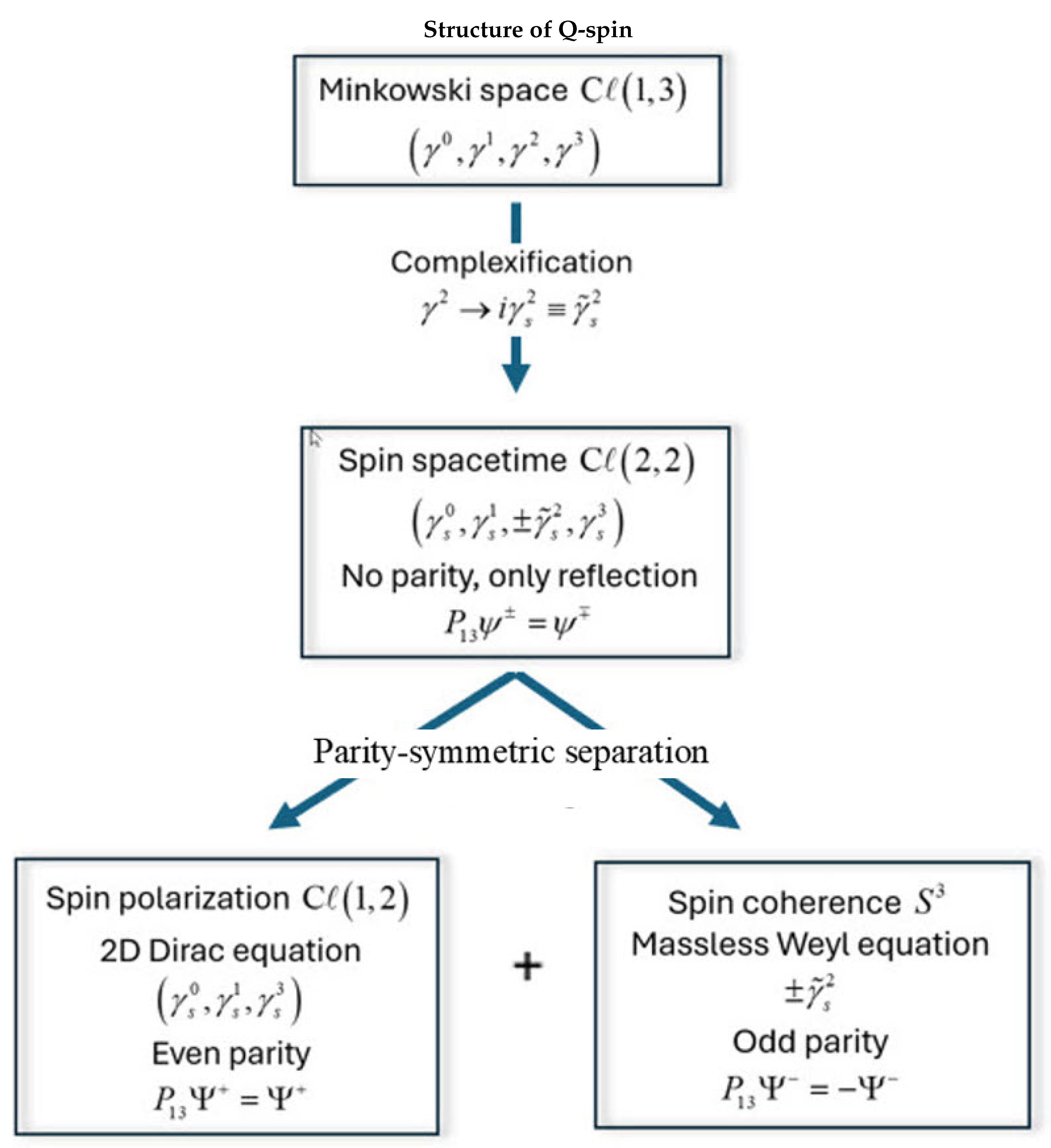
Appendix B Quantum Correspondence
For completeness, we summarize the QFT treatment of a quantum bivector to show the classical treatment is faithfully followed by the quantum. Without details, [3], Figure A1), the usual Dirac equation, top panel, obeys the Clifford algebra of Minkowski space, , with three spatial components and one time. Introducing the bivector renders the Dirac equation non-Hermitian, with : two time components (linear and helical period) and two spatial axes forming a disc. Its two solutions are the mirror states , Equation (20), which are complex conjugates and denote opposite chirality. Under parity, the non-Hermiticity separates into two complementary equations: a two-dimensional Dirac equation describing the even-parity disc and a massless Weyl equation of odd parity describing helicity as a quaternion [3]. This approach is consistent with Twistor Theory [99,100], which complexifies Minkowski space by replacing the four real parameters with complex forms. Twistor space, T, is projected into two helicity spaces, . Here, we take the Dirac field D, complexify it to , and then use to project out the two helicity states [3,4].
Appendix C Symmetry of Quaternion Spin
The standard Dirac equation represents spin through complex four-component spinors, invoking the symmetry group . These spinor components, , each with components of opposite chiralities, are mirror images under parity, Equation (21), and are interpreted as a matter–antimatter pair.
The anti-commutation relations are satisfied by quaternion gamma matrices, , which are also constructed using skew-diagonal Pauli components. These are real matrices, , and their algebra forms the discrete quaternion group , which is isomorphic to the continuous group of unit quaternions, , under multiplication, [101,102,103]. In the BiSM, spinor algebra is replaced by quaternionic geometry.
In analogy with the Dirac case, the symmetry is replaced by the real algebra , defined as the group of real matrices with determinant . The full symmetry structure is then , where each matrix represents one of the two orthogonal planes associated with each blade. This replaces the chiral spinor components in the SM with geometric planes with definite internal dynamics in the BiSM.
References
- Peskin, M.; Schroeder, D.V. An Introduction To Quantum Field Theory; Frontiers in Physics: Boulder, CO, USA, 1995. [Google Scholar]
- Dirac, P.A.M. The quantum theory of the electron. Proceedings of the Royal Society of London. Series A, Containing Papers of a Mathematical and Physical Character, 1928; 117, 610–624. [Google Scholar]
- Sanctuary, B. Quaternion Spin. Mathematics 2024, 12, 1962. [Google Scholar] [CrossRef]
- Sanctuary, B. Spin Helicity and the Disproof of Bell’s Theorem. Quantum Rep. 2024, 6, 436–441. [Google Scholar] [CrossRef]
- Sanctuary, B. EPR Correlations Using Quaternion Spin. Quantum Rep. 2024, 6(3), 409–425. [Google Scholar] [CrossRef]
- Doran, C.; Lasenby, J. Geometric algebra for physicists; Cambridge University Press, 2003. [Google Scholar]
- Dirac, P.A.M. A Theory of Electrons and Protons. Proc. R. Soc. Lond. A. 1930, 126(801), 360–365. [Google Scholar]
- Greiner, W. Relativistic Quantum Mechanics-Wave Equations; SpringerVerlag: Berlin, Germany, 2000; pp. 310–360. [Google Scholar]
- Paganini, P. Fundamentals of particle physics: understanding the standard model; Cambridge University Press, 2023. [Google Scholar]
- Skyrme, T.H.R. A unified field theory of mesons and baryons. Nuclear Physics 1962, 31, 556–569. [Google Scholar] [CrossRef]
- Pezzaglia, W.M. Physical applications of a generalized Clifford calculus (Papapetrou equations and metamorphic curvature). arXiv 1997, preprint gr-qc/9710027.
- Hestenes, D. Spin and uncertainty in the interpretation of quantum mechanics. American Journal of Physics 1979, 47, 399–415. [Google Scholar] [CrossRef]
- Hestenes, D.; Sobczyk, G. Clifford algebra to geometric calculus: a unified language for mathematics and physics (Vol. 5); Springer Science and Business Media, 2012. [Google Scholar]
- Nash, C.; Sen, S. Topology and geometry for physicists; Elsevier, 1988. [Google Scholar]
- Schwarz, A.S. Quantum field theory and topology (Vol. 307); Springer Science and Business Media: 2013.
- Hestenes, D. The zitterbewegung interpretation of quantum mechanics. Foundations of Physics 1990, 20(10), 1213–1232. [Google Scholar] [CrossRef]
- Muralidhar, K. The spin bivector and zeropoint energy in geometric algebra. Adv. Studies Theor. Phys 2012, 6, 675–686. [Google Scholar]
- Goldstein, H. Classical mechanics; Pearson Education India, 2011. [Google Scholar]
- Carroll, S.M. Spacetime and geometry; Cambridge University Press, 2019. [Google Scholar]
- Leonard, I.E.; Lewis, J.E. Geometry of convex sets; John Wiley and Sons, 2015. [Google Scholar]
- Hadwiger, H. Minkowskische addition und subtraktion beliebiger punktmengen und die theoreme von erhard schmidt. Mathematische Zeitschrift 1950, 53(3), 210–218. [Google Scholar] [CrossRef]
- Bell, J.S. On the Einstein Podolsky Rosen paradox. Physics Physique Fizika 1964, 1, 195. [Google Scholar] [CrossRef]
- Bell, J.S. Speakable and unspeakable in quantum mechanics; Cambridge University Press: New York, 1987. [Google Scholar]
- Brunner, N.; Cavalcanti, D.; Pironio, S.; Scarani, V.; Wehner, S. Bell nonlocality. Reviews of modern physics 2014, 86(2), 419–478. [Google Scholar] [CrossRef]
- Clauser, J.F.; Horne, M.A.; Shimony, A.; Holt, R.A. Proposed experiment to test local hidden-variable theories. Physical review letters 1969, 23(15), 880. [Google Scholar] [CrossRef]
- Aspect, A.; Dalibard, J.; Roger, G. Experimental test of Bell’s inequalities using time-varying analyzers. Physical review letters 1982, 49, 1804.Aspect, A. Proposed experiment to test the non separability of quantum mechanics. Physical Review D 1976, 14, 1944–1951. [Google Scholar] [CrossRef]
- Weihs, G.; Jennewein, T.; Simon, C.; Weinfurter, H.; Zeilinger, A. Violation of Bell’s inequality under strict Einstein locality conditions. Physical Review Letters 1998, 81(23), 5039. [Google Scholar] [CrossRef]
- Wiseman, H.M. The two Bell’s theorems of John Bell. Journal of Physics A: Mathematical and Theoretical 2014, 47, 424001. [Google Scholar] [CrossRef]
- Kupczynski, M. Quantum nonlocality: how does nature do it? Entropy 2024, 26(3), 191. [Google Scholar] [CrossRef]
- Wilczek, F. Quantum mechanics of fractional-spin particles. Physical review letters 1982, 49(14), 957. [Google Scholar] [CrossRef]
- Khrennikov, A. Contextual approach to quantum mechanics and the theory of the fundamental prespace. arXiv 2003, preprint quant-ph/0306003.
- Khrennikov, A. Y. Contextual approach to quantum formalism (Vol. 160); Springer Science & Business Media: 2009.
- Hestenes, D.; Lasenby, A. Space-time algebra; Springer International Publishing: Switzerland, 2015; p. 2015. [Google Scholar]
- Berry, M.V. (1984). Quantal phase factors accompanying adiabatic changes. Proceedings of the Royal Society of London. A. Mathematical and Physical Sciences 1802, 392, 45–57. [Google Scholar]
- Oveshnikov, L. N., Kulbachinskii, V. A., Davydov, A. B., Aronzon, B. A., Rozhansky, I. V., Averkiev, N. S., ...; Tripathi, V. Berry phase mechanism of the anomalous Hall effect in a disordered two-dimensional magnetic semiconductor structure. Scientific reports 2015, 5, 17158. [Google Scholar] [CrossRef]
- Skrynnikov, N. R.; Sanctuary, B. C. Geometric phase in NMR interferometry experiment. Molecular Physics 1994, 83(6), 1133–1144. [Google Scholar] [CrossRef]
- Schwinger, J. Quantum electrodynamics. I. A covariant formulation. Physical Review 1948, 74(10), 1439. [Google Scholar] [CrossRef]
- Feynman, R. P. Space-time approach to quantum electrodynamics. In Quantum Electrodynamics; CRC Press, 2018. [Google Scholar]
- Dyson, F. J. The Radiation Theories of Tomonaga, Schwinger, and Feynman. Phys. Rev. 1949, 75, 486. [Google Scholar] [CrossRef]
- Gell-Mann, M.,; Low, F. E. Quantum electrodynamics at small distances. Physical Review 1954, 95(5), 1300. [Google Scholar] [CrossRef]
- Wilson, K. G. Renormalization group and critical phenomena. I. Renormalization group and the Kadanoff scaling picture. I. Renormalization group and the Kadanoff scaling picture. Physical review B 1971, 4(9), 3174. [Google Scholar] [CrossRef]
- Wilson, K. G. , & Kogut, J. The renormalization group and the epsilon expansion. The renormalization group and the epsilon expansion. Physics reports 1974, 12(2), 75–199. [Google Scholar]
- Gross, D. J. Twenty five years of asymptotic freedom. Nuclear Physics B-Proceedings Supplements 1999, 74, 426–446. [Google Scholar] [CrossRef]
- Sanyuk, V. I.,; Sukhanov, A. D. Dirac in 20th century physics: a centenary assessment. Physics-Uspekhi 2003, 46, 937. [Google Scholar] [CrossRef]
- Sanctuary, Bryan, "Qubits, Beta decay and Parity", 2025, In preparation.
- Coope, J. A. R.; Snider, R. F.; McCourt, F. R. Irreducible cartesian tensors. The Journal of Chemical Physics 1965, 43(7), 2269–2275. [Google Scholar] [CrossRef]
- Coope, J. A. R., and Snider, R. F. Irreducible cartesian tensors. II. General formulation. Journal of Mathematical Physics 1970, 11(3), 1003–1017. [Google Scholar] [CrossRef]
- Coope, J. A. R. Irreducible Cartesian Tensors. III. Clebsch-Gordan Reduction. Journal of Mathematical Physics 1970, 11, 1591–1612. [Google Scholar] [CrossRef]
- Snider, R.F. Irreducible Cartesian Tensors (Vol. 43); Walter de Gruyter GmbH and Co KG, 2017. [Google Scholar]
- Kalb, M.; Ramond, P. Classical direct interstring action. Physical Review D 1974, 9(8), 2273. [Google Scholar] [CrossRef]
- Jackson, J.D. Classical electrodynamics; John Wiley & Sons, 2021. [Google Scholar]
- https://en.wikipedia.org/wiki/Pauli_matrices.
- Frankel, T. The geometry of physics: an introduction; Cambridge university press, 2011. [Google Scholar]
- Ryder, L.H. Quantum field theory; Cambridge university press, 1996. [Google Scholar]
- Donoghue, J. F.; Golowich, E.; Holstein, B. R. Dynamics of the standard model; Cambridge university press, 2014; p. 573. [Google Scholar]
- Sanctuary, B. Quaternion spin: parity and beta decay, 2025.
- Mohapatra, R.N.; Pal, P.B. Massive neutrinos in physics and astrophysics; World scientific, 2004; Vol. 72. [Google Scholar]
- Altarelli, G. The mystery of neutrino mixings. arXiv 2011, preprint arXiv:1111.6421.
- Born, M.; Oppenheimer, R. (2000). On the quantum theory of molecules. In Quantum Chemistry: Classic Scientific Papers (pp. 1-24).
- Donoghue, J. F.; Golowich, E.; Holstein, B. R. Dynamics of the standard model; Cambridge university press, 2014; p. 573. [Google Scholar]
- Zee, A. Quantum Field Theory in a Nutshell; Princeton University Press, 2010. [Google Scholar]
- Fano, U. Description of states in quantum mechanics by density matrix and operator techniques. Reviews of modern physics 1957, 29(1), 74. [Google Scholar] [CrossRef]
- Von Neumann, John. Mathematical foundations of quantum mechanics. Princeton university press, 1955.
- Wilde, M. M. (2013). Quantum information theory. Cambridge university press.
- Fields, B.; Sarkar, S. Big-bang nucleosynthesis (particle data group mini-review). arXiv 2006, preprint astro-ph/0601514.
- Peres, A. (Ed.). (2002). Quantum theory: concepts and methods. Dordrecht: Springer Netherlands.
- Hu, X. M.; Guo, Y.; Liu, B. H.; Li, C. F.; Guo, G. C. Progress in quantum teleportation. Nature Reviews Physics 2023, 5(6), 339–353. [Google Scholar] [CrossRef]
- Bennett, C. H.; Brassard, G.; Crépeau, C.; Jozsa, R.; Peres, A.; Wootters, W. K. Teleporting an unknown quantum state via dual classical and Einstein-Podolsky-Rosen channels. Physical review letters 1993, 70(13), 1895. [Google Scholar] [CrossRef]
- P. W. Shor, “Algorithms for quantum computation: Discrete logarithms and factoring,” in Proceedings of the 35th Annual Symposium on Foundations of Computer Science (FOCS), pp. 124–134, IEEE, 1994.
- Levitt, M. H. (2008). Spin dynamics: basics of nuclear magnetic resonance. John Wiley & Sons.
- Edmonds, A. R. (1996). Angular momentum in quantum mechanics (Vol. 4). Princeton university press.
- Guessoum, N.; Jean, P.; Gillard, W. The lives and deaths of positrons in the interstellar medium. Astronomy & Astrophysics, 2005; 436, 171–185. [Google Scholar]
- Weidenspointner, G.; Skinner, G.; Jean, P.; Knödlseder, J.; Von Ballmoos, P.; Bignami, G.; ...; Winkler, C. An asymmetric distribution of positrons in the Galactic disk revealed by gamma-rays. Nature, 2008; 451, 159–162. [Google Scholar]
- Beacom, J. F.; Bell, N. F.; Bertone, G. Gamma-ray constraint on Galactic positron production by MeV dark matter. Physical Review Letters 2005, 94(17), 171301. [Google Scholar] [CrossRef]
- Celso, J. Villas-Boas, Carlos E. Máximo, Paulo J. Paulino, Romain P. Bachelard, and Gerhard Rempe. ’Bright and Dark States of Light: The Quantum Origin of Classical Interference. Phys. Rev. Lett. 2024, 134, 133603. [Google Scholar] [CrossRef]
- Steinberg, A. M. (2014). Quantum Measurements: a modern view for quantum optics experimentalists.
- Whitesides, G. M.; Grzybowski, B. Self-assembly at all scales. Science 2002, 295(5564), 2418–2421. [Google Scholar] [CrossRef]
- Griffiths, D. (2020). Introduction to elementary particles. John Wiley & Sons.
- Laurikainen, K. V. (2012). Beyond the atom: the philosophical thought of Wolfgang Pauli. Springer Science & Business Media.
- Wu, C. S.; Ambler, E.; Hayward, R. W.; Hoppes, D. D.; Hudson, R. P. Experimental test of parity conservation in beta decay. Physical review 1957, 105(4), 1413. [Google Scholar] [CrossRef]
- Doherty, M. W.; Manson, N. B.; Delaney, P.; Jelezko, F.; Wrachtrup, J.; Hollenberg, L. C. The nitrogen-vacancy colour centre in diamond. Physics Reports 2013, 528(1), 1–45. [Google Scholar] [CrossRef]
- aylor, J. M.; Cappellaro, P.; Childress, L.; Jiang, L.; Budker, D.; Hemmer, P. R.; ...; Lukin, M. D. High-sensitivity diamond magnetometer with nanoscale resolution. Nature Physics 2008, 4(10), 810–816. [Google Scholar] [CrossRef]
- Abi, B.; Albahri, T.; Al-Kilani, S.; Allspach, D.; Alonzi, L. P.; Anastasi, A.; ...; Lusiani, A. Measurement of the positive muon anomalous magnetic moment to 0.46 ppm. Physical Review Letters 2021, 126(14), 141801. [Google Scholar] [CrossRef]
- Aoyama, T.; Asmussen, N.; Benayoun, M.; Bijnens, J.; Blum, T.; Bruno, M. .. ; Zhevlakov, A. S. The anomalous magnetic moment of the muon in the Standard Model. Physics reports 2020, 887, 1–166. [Google Scholar] [CrossRef]
- Moroi, T. Muon anomalous magnetic dipole moment in the minimal supersymmetric standard model. Physical Review D 1996, 53(11), 6565. [Google Scholar] [CrossRef]
- Gabrielse, G.; et al. New Determination of the Fine Structure Constant from the Electron g Value and QED. Phys. Rev. Lett. 2006, 97, 030802. [Google Scholar] [CrossRef] [PubMed]
- P. J. Mohr, B. N. Taylor, and D. B. Newell. CODATA Recommended Values of the Fundamental Physical Constants. Rev. Mod. Phys. 2012, 84, 1527. [Google Scholar] [CrossRef]
- KATRIN Collaboration†, Aker, M., Batzler, D., Beglarian, A., Behrens, J., Beisenkötter, J.,; Zeller, G. Direct neutrino-mass measurement based on 259 days of KATRIN data. Science, 2025; 388, 180–185. [Google Scholar]
- Eguchi, K., Enomoto, S., Furuno, K., Goldman, J., Hanada, H., Ikeda, H., ...; (KamLAND Collaboration). First results from KamLAND: evidence for reactor antineutrino disappearance. Physical review letters 2003, 90, 021802. [Google Scholar] [CrossRef]
- Freitas, A. TASI 2020 lectures on precision tests of the standard model. arXiv 2020, preprint arXiv:2012.11642.
- Erler, J.; Schott, M. Electroweak precision tests of the Standard Model after the discovery of the Higgs boson. Progress in Particle and Nuclear Physics 2019, 106, 68–119. [Google Scholar] [CrossRef]
- Fan, X.; Myers, T.G.; Sukra, B.A.D.; Gabrielse, G. Measurement of the electron magnetic moment. Physical review letters 2023, 130(7), 071801. [Google Scholar] [CrossRef]
- Lamb, W.E.; Retherford, R.C. Fine Structure of the Hydrogen Atom by a Microwave Method. Phys. Rev. 1947, 72, 241. [Google Scholar] [CrossRef]
- Casimir, H. B. G. On the Attraction Between Two Perfectly Conducting Plates. Proc. K. Ned. Akad. Wet. 1948, 51, 793. [Google Scholar]
- Wikipedia: Physics beyond the Standard Model, accessed April 2025.
- "Interpretations of quantum mechanics," Wikipedia, The Free Encyclopedia, [Online]. Available: urlhttps://en.wikipedia.org/wiki/Interpretations of quantum mechanics. [2025-04-05].
- Werner Heisenberg. Über den anschaulichen Inhalt der quantentheoretischen Kinematik und Mechanik. Zeitschrift für Physik 1927, 43, 172–198. English translation: “The Physical Content of Quantum Kinematics and Mechanics,” in Quantum Theory and Measurement, edited by J. A. Wheeler and W. H. Zurek (Princeton University Press, 1983), pp. 62–8.
- Lee, T. D.; Yang, C. N. Question of parity conservation in weak interactions. Physical Review 1956, 104(1), 254. [Google Scholar] [CrossRef]
- Penrose, R. Twistor algebra. Journal of Mathematical Physics 1967, 8, 345–366. [Google Scholar] [CrossRef]
- Penrose, R. Solutions of the Zero-Rest-Mass Equations. Journal of Mathematical Physics 1969, 10, 38–39. [Google Scholar] [CrossRef]
- Hall, B.C. Lie groups, Lie algebras, and representations. In Quantum Theory for Mathematicians; Springer New York: New York, NY, USA, 2013; pp. 333–366. [Google Scholar]
- Howard Georgi – Lie Algebras in Particle Physics.
- Cornwell, J. F. (1984). Group theory in physics. Academic Press.
Figure 1.
Left: Dirac’s matter-antimatter pair of the SM. Right: The BiSM showing two counter precessing angular momentum cones on the same particle which form a bivector.
Figure 1.
Left: Dirac’s matter-antimatter pair of the SM. Right: The BiSM showing two counter precessing angular momentum cones on the same particle which form a bivector.
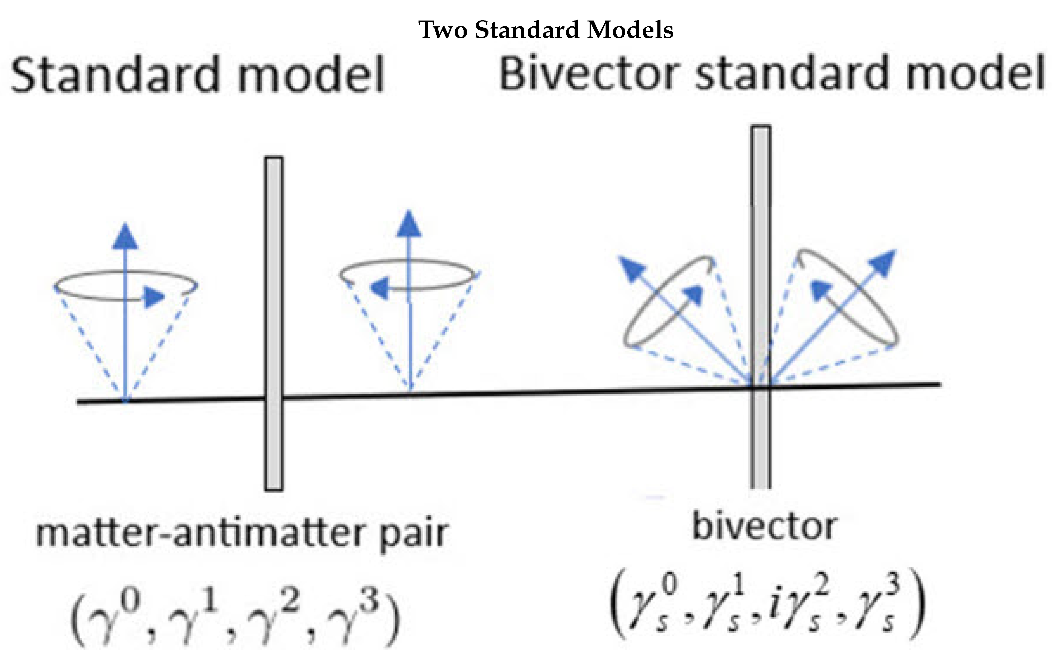
Figure 2.
Three views of a spinning object: Left: a point particle with spin (LFF), Middle: a disc with vector motion (LFF), and Right: a classical bivector with internal motion (BFF). In the LFF, the angular momentum is intrinsic, being the projection of the internal bivector motion that is in the BFF which is unobservable.
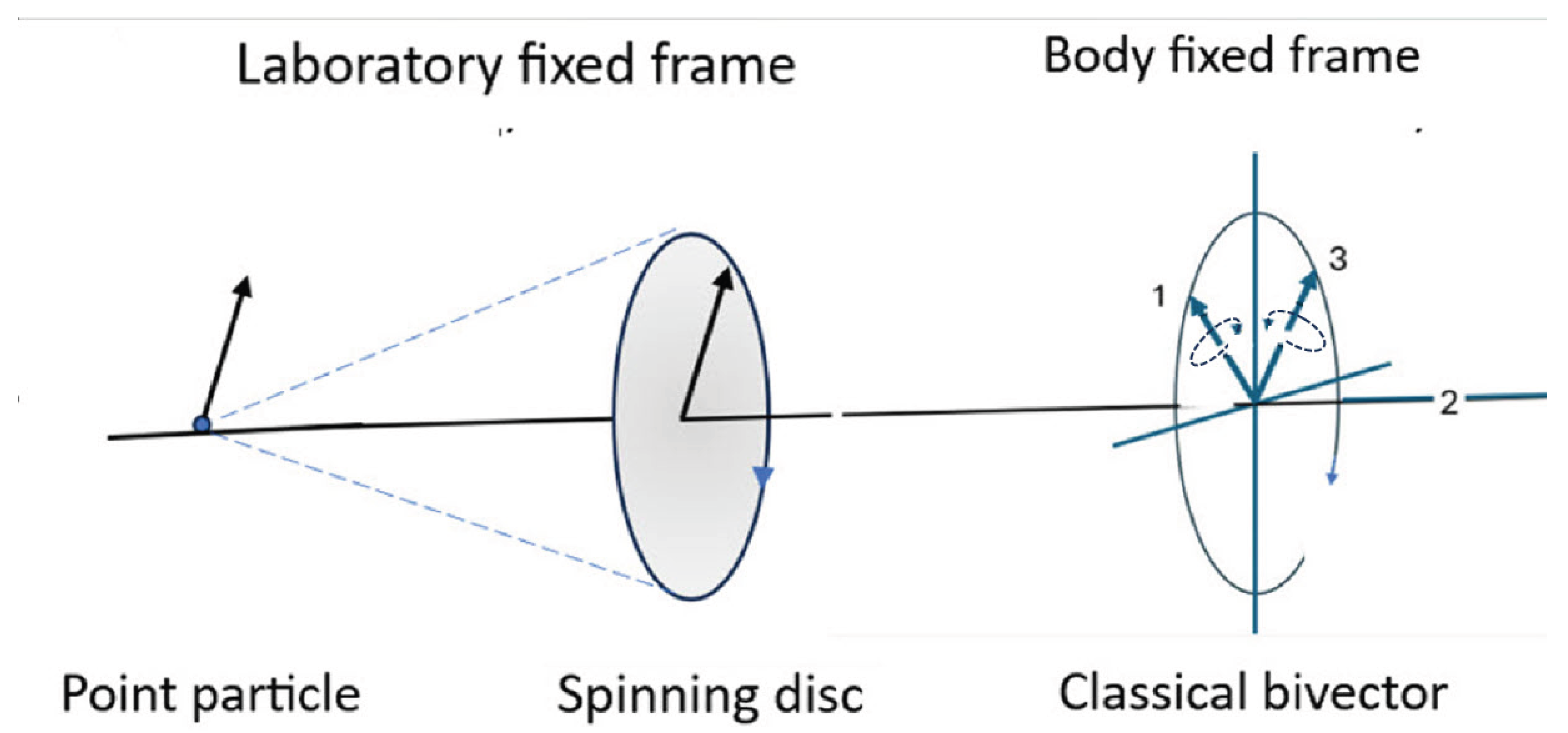
Figure 3.
Classical spin bifurcation. Right: A classical bivector with two orthogonal massive axes, 1 and 3, spinning about axis 2 (projecting out of the page). Center: The two mirror-image precession states, , represent Nature’s left and right hands. The angles between axes 1 and 3 and their angular momentum vectors are equal in both states and increase with precession frequency. A mirror plane bisects the 1–3 axes. At , the classical spin magnitude is , corresponding to a spin-1 boson. Right: The cone is decomposed into components and , orthogonal and parallel to the precession axis. Bottom: Left: Quantum state of even parity showing the loss of reflection within the double helix of mass along the bisector, 31. Right: Permuting the 1 and 3 labels reverses the handedness of the frame. Summing the two frames cancels the torques; subtracting them cancels matter. Matter and force are separated.
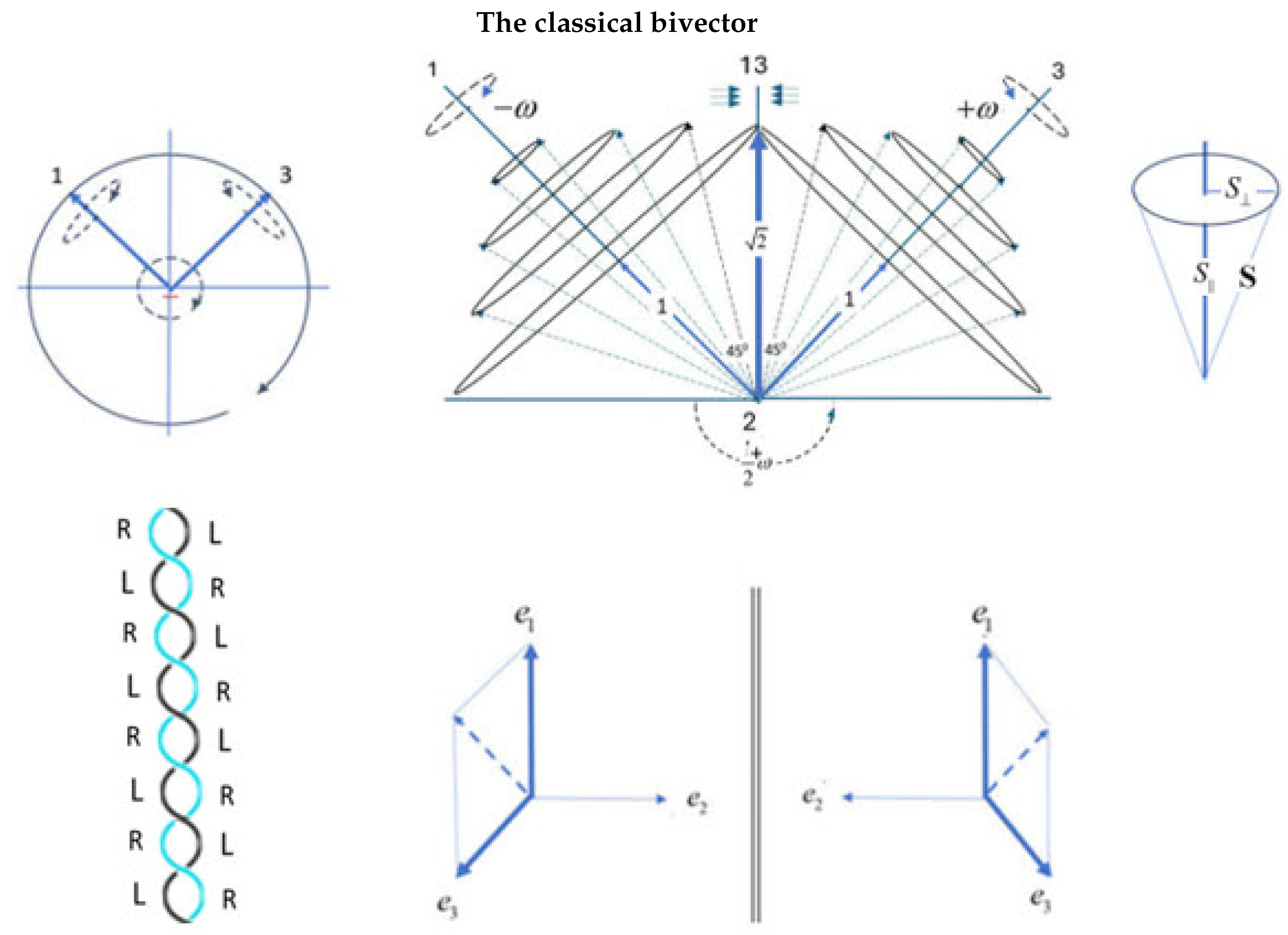
Figure 4.
Plotting EPR correlation versus the angle difference . The points give the results of the simulation. The CHSH values are listed and the full correlation is the sum of polarization, (the triangle) and the coherence, (the mustache). Note the hardly discernible residual polarization correlation along the horizontal axis, which shows the contribution extracted from the polarization, .
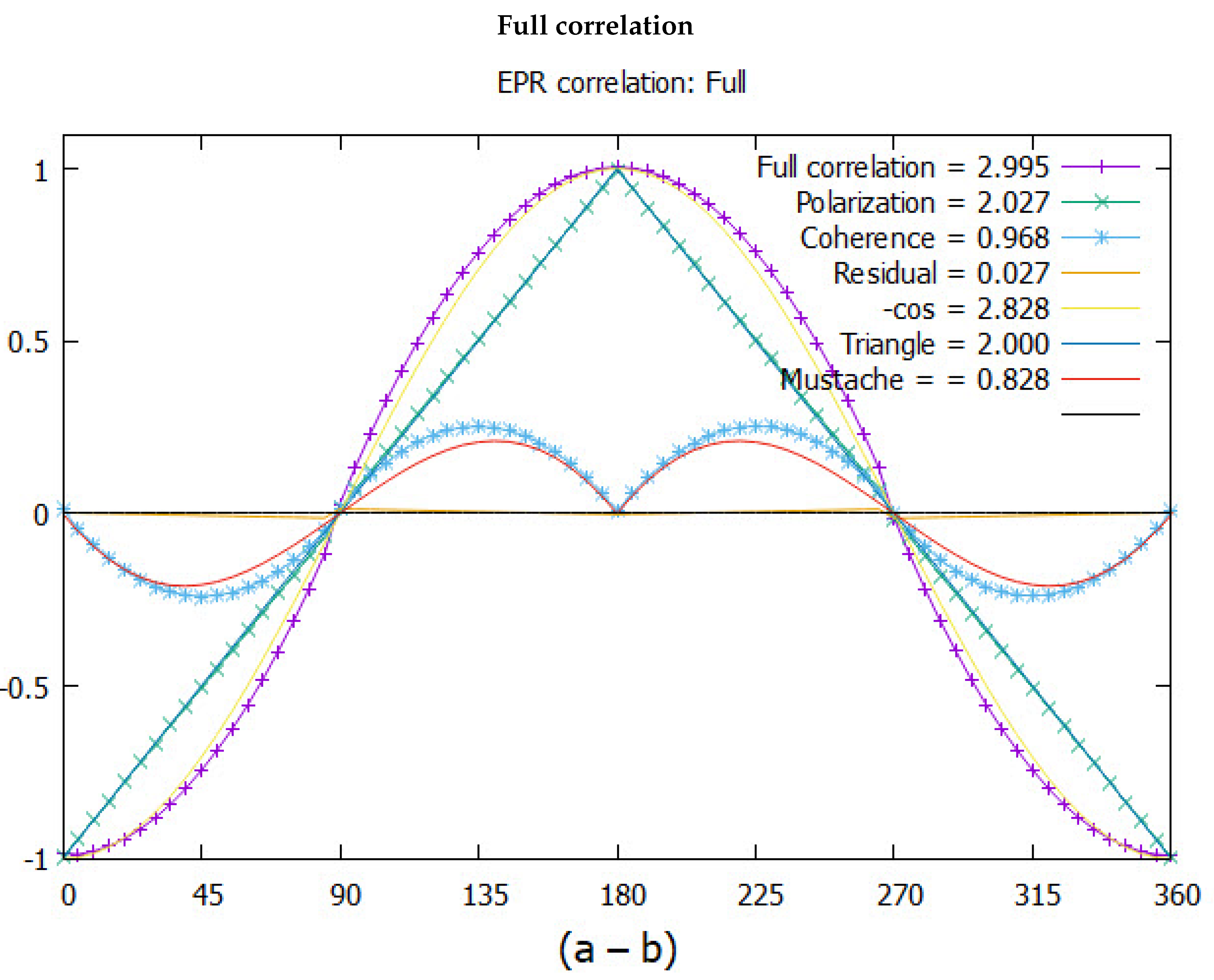
Figure 5.
Three manifestations of bosons: When the incoming boson and the target have opposite chirality, they meld into matter of even parity. When their chiralities are equal, they combine to create a greater torque of odd parity. These require the polarizing field be outside the 13 interaction plane. If the polarizing field lands within the interaction plane, 31, then a massive quantum impinges on the surface with no chirality. The long arrows denote two positions of the polarizing field vector: one in the interaction plane and the other outside of it.
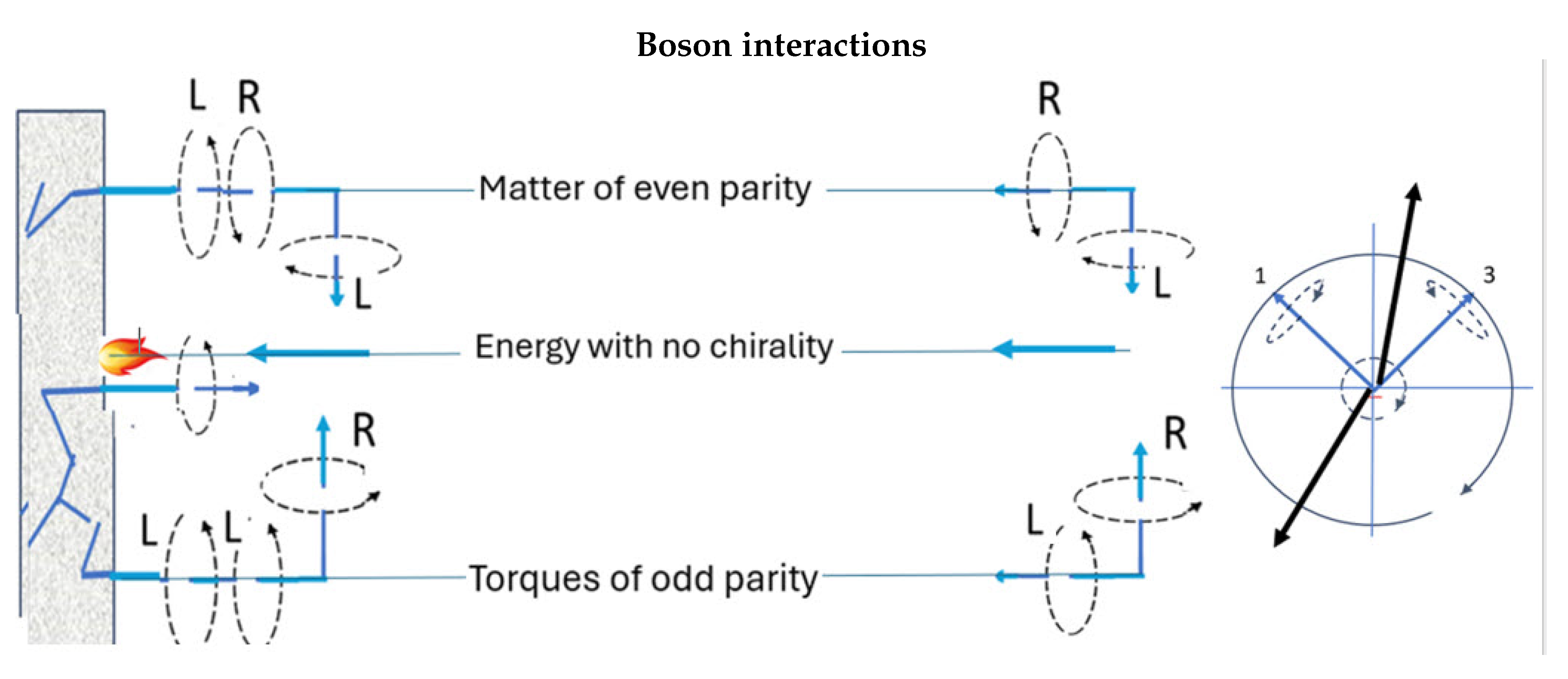
Figure 6.
Left: Spinor-based SU(2) construction of higher spins. Right: Vector-based construction using SO(3) symmetric traceless tensors
Figure 6.
Left: Spinor-based SU(2) construction of higher spins. Right: Vector-based construction using SO(3) symmetric traceless tensors
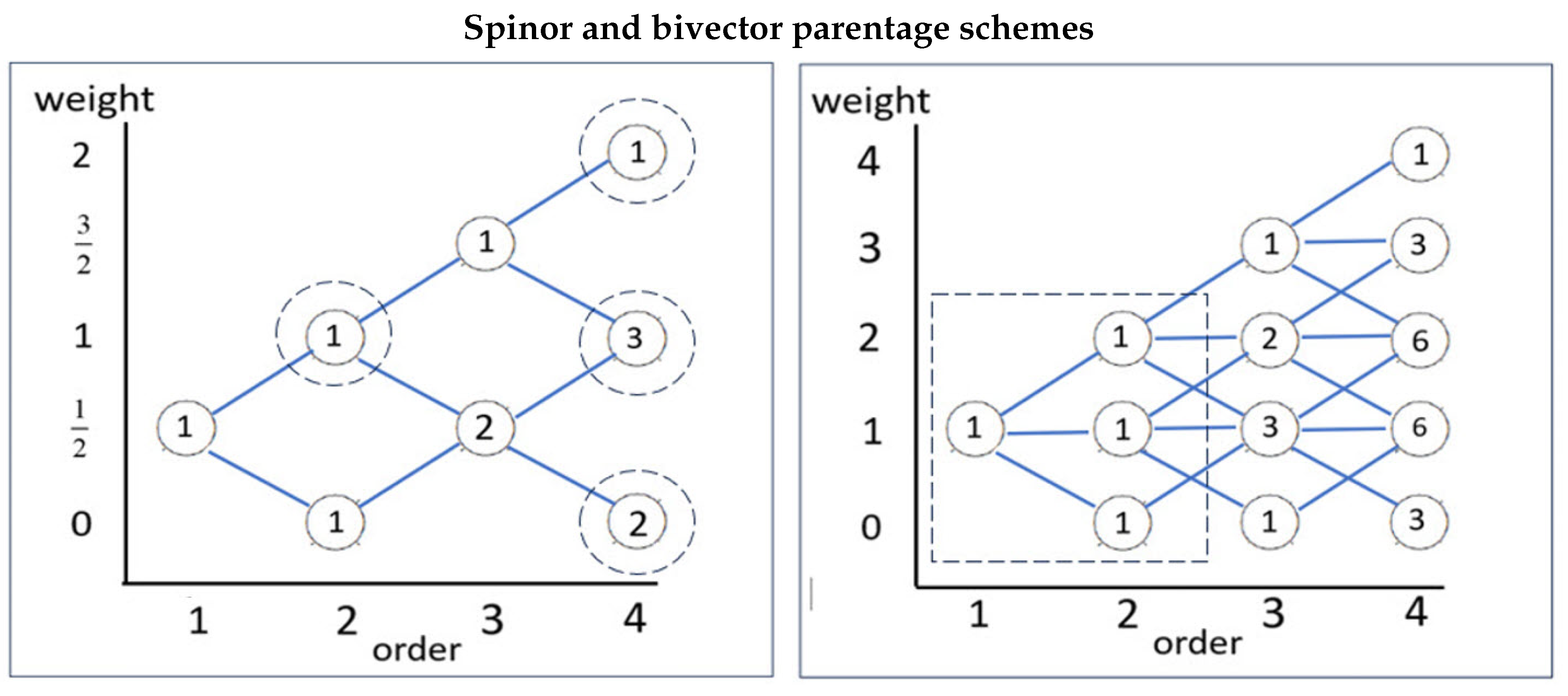
Figure 7.
Geometric structures by combining bivectors.
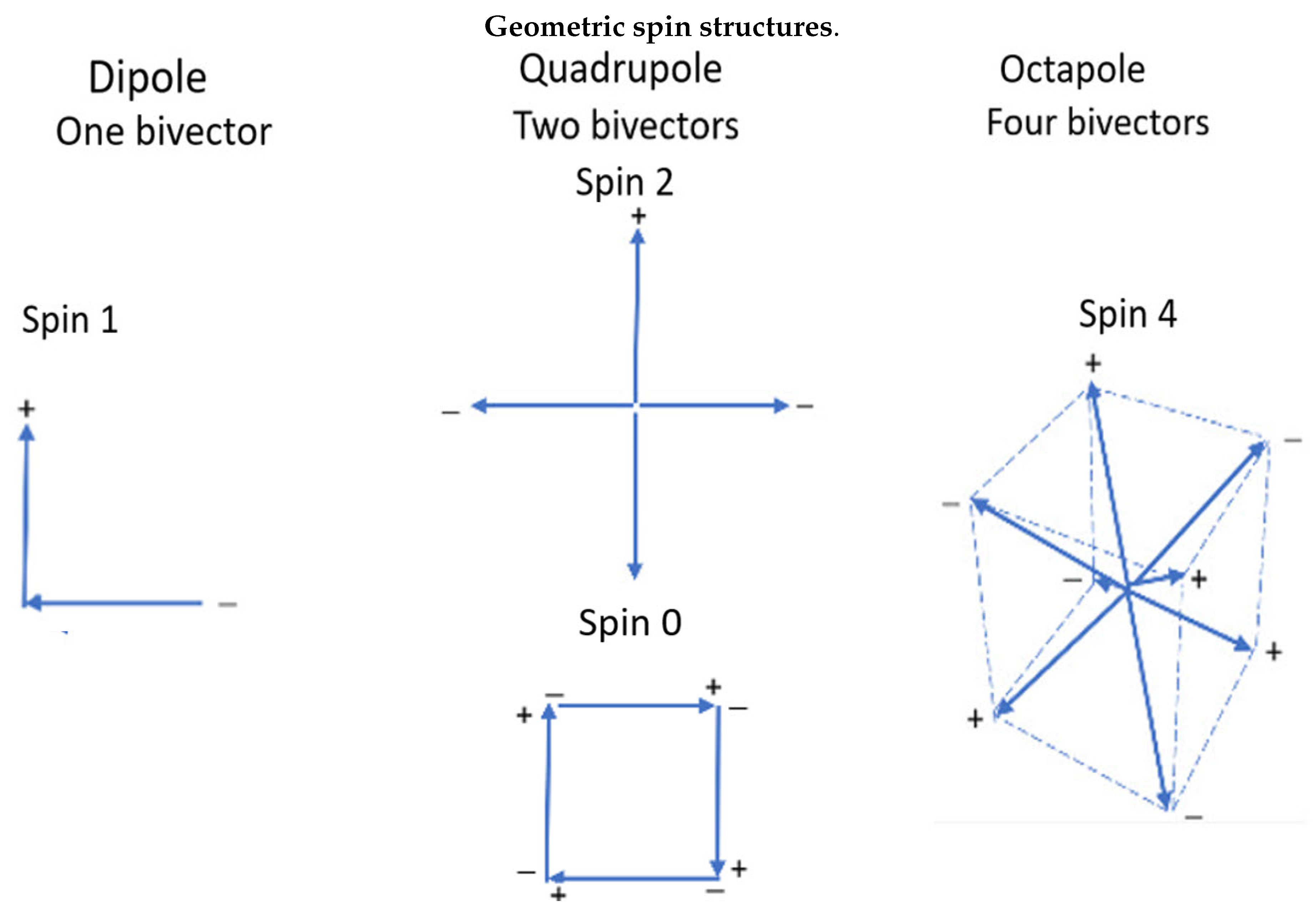
Disclaimer/Publisher’s Note: The statements, opinions and data contained in all publications are solely those of the individual author(s) and contributor(s) and not of MDPI and/or the editor(s). MDPI and/or the editor(s) disclaim responsibility for any injury to people or property resulting from any ideas, methods, instructions or products referred to in the content. |
© 2025 by the authors. Licensee MDPI, Basel, Switzerland. This article is an open access article distributed under the terms and conditions of the Creative Commons Attribution (CC BY) license (http://creativecommons.org/licenses/by/4.0/).
Copyright: This open access article is published under a Creative Commons CC BY 4.0 license, which permit the free download, distribution, and reuse, provided that the author and preprint are cited in any reuse.


