
Submitted:
10 August 2025
Posted:
11 August 2025
You are already at the latest version
Abstract
Using a bivector model of quantum spin, and only Classical Mechanics and Special Relativity, we find the correspondence between the classical and quantum domains. Spinning to relativistic velocities reveals a symmetry change where classical reflection becomes quantum parity.
Keywords:
quaternion spin
; dirac field
; quantum coherence
; wave-particle duality
; neutrinos
; parity
; anyons
; Twistor theory
; quantum theory
1. Introduction
Complementary pairs: energy-time; momentum-position; angular momentum-angle have classical correspondence as Planck’s constant becomes negligible. Spin is different. It is postulated as a purely quantum property of intrinsic angular momentum with no classical correspondence. In this paper, we show that correspondence exists. By using a classical model of spin, space bifurcates into the quantum domain of parity at large but not relativistic velocities of precessing cone rim, ..
We first discuss a classical bivector using classical mechanics, showing that all the properties of quantum spin are faithfully obtained. We find that as a bivector spins faster, its two angular momenta combine into a double helix of mass inside their mirror plane. There reflection is lost and the even state of parity is defined. This is the quantum state, where classical becomes quantum, giving the classical-quantum correspondence for spin.
This work was motivated by the EPR paradox, [1,2,3,4,5,6,7], by showing the violation of Bell’s Inequalities, [8], is due to quantum coherence from a bivector. Our modified definition of spin angular momentum,
includes the geometric helicity which is a bivector defined by,
As a result, rather than spin polarization, , we have a unit quaternion, . Here describes the polarizing field. This formulation led to modeling Equation (1) as a classical bivector, and the results strongly supports this structure for Q-spin.
2. Classical Spin-1 Boson
The bivector structure shown in the left panel of Figure 1 depicts a bivector with external vector precession. The two massive orthogonal axes of the bivector are labeled 1 and 3. In response to the vector motion around the massless axis 2, these two axes counter-precess with opposite angular velocities, . Take the moment of inertia for the external vector as , and that for the internal bivector as . The bivector axes counter precess at twice the frequency of the torque axis, 2, and therefore the rotational energies, , for the disc and the two axes, are distributed between the vector and bivector in the ratio,
a ratio maintained for any precessional frequency of a rigid bivector. As the massless 2 axis turns, it generates a disc and drives the bivector. When there are no external torques the system is conservative, so Euler’s equations use the substantive derivative, [9],
where is the angular momentum of the rigid body, and is the angular velocity. With the 2-axis massless, there are two independent equations, one for each axis,
. Conservation of energy and angular momentum leads to cones around each axis which precess in tandem, and maintain their mirror reflection. Their interaction plane, 13, is where the two cones are closest and furthest in their orbits, giving,
These are shown at various angles , defined as that between an axis, and the vector, , Figure 1. The units are radians per second, and G is a gauge to be determined by the system. The period of precessions is . These components are normalized: parallel to the axes is ; and perpendicular to the axis is , Figure 1.
The counter precessing cones of angular momentum, Figure 1, lead to the definition of classical spin as a bivector being the wedge product of the two angular momenta associated with each axis, [10],
thereby defining their interaction plane, 13. Using Equation (6), the scalar and the wedge products are,
Here we introduce , which is the angle between the two angular momentum vectors, and related by . Normalized gives a unit quaternion structure of a scalar and bivector which we express as the geometric product, [10], of the two angular momenta,
Classical spin is a bivector, Equation (7), and the geometric product, Equation (9), describes its dynamics as a classical rotor.
The unit vector is normal to the 31 plane and gives rotation around the 2 axis which is manifest in the Laboratory Fixed Frame, LFF, in Minkowski space, . There it is a spinning disc. This quaternion also gives a measure of scalar and bivector contributions at different angles. The scalar part gives a measure of its mass, and the bivector part gives coherent rotational kinetic energy from the two counter precessing axes. At , the scalar part is maximized to 1, and the two axes 1, 3, meld which cancels their precessions, leaving scalar mass. Equation (3) shows that the ratio of the rotational kinetic energies is fixed. As the internal frequency goes to zero, so the external precession slows and stops. In isotropy, all kinetic energy is converted to mass, which is the only property it displays. It is still a bivector. We call this the Body Fixed Frame, BFF, denoted by ), the rest frame, and the mass the rest mass. We identify this maximally confined structure to have the classical electron radius . We refer to this as an inert electron.
3. The Double Helix of Mass
When , the two angular momentum intertwine along their mirror plane, and form a double helix, Figure 1. This classical angular momentum has no physical axis and is a purely resonant state: the eye of a tornado along 13. The analogy is apt but with an extra twist. The eye of a vector tornado is a region of calm and lower energy, yet surrounded by a vortex of high precessional energy. In contrast, the bivector tornado is due the two axes melding into an eye of left and right chiralities intertwined in harmony, Figure 1. There is no vortex, only a scalar directed along the bisector with calm everywhere else. It is the double helix of the electron. Therein Nature stores its defining properties. At , we assign this state the magnetic classical number . The two blades, Equation (7), , have folded together. Figure 1 shows how reflection is lost and all opposite blade properties cancel. This depicts the quantum state of the electron which exists at .
When an electron in state encounters a polarizing field, its properties of spin (chirality), helicity, charge and mass emerge as we observe. The two blades are forced into a polarizing state of , that is indistinguishable from a fermion.
The quaternion, , is also a phase which changes sign when 1 and 3 labels are swapped. This symmetry operation shows the 1 and 3 labels are indistinguishable, allowing for both the clockwise and counter clockwise helicity around the 2 axis.
4. A Classical Boson of Spin-1
This resonant and scalar state is formed from the coherent coupling of the two perpendicular components, , one from axis-3 and one from axis-1. As seen from Figure 1, the component from axis-1, , projects onto the 23 plane, while the axis-3 component projects onto the 12 plane. Any cone will give a spin-1, but the maximum value occurs when at . We normalize these cone projections and the angle between the projected component and the bisector, 31, is . A spin is formed from these two components which resonates giving a state of length . Using the quantum definition for the angle, , between a spin axis and its cone, we get
which is identified as a purely classical spin 1. Moreover, this particle is rapidly spinning, averaging out all anisotropies, and obeying Bose-Einstein statistics. We are justified in calling the classical spin a boson. Since the spin-1 is a result of the coupling of the two blades, we assign a spin of to , and .
5. Special Relativity
Using the angular momentum of an electron, , its mass, and a radius defined by the de Broglie wavelength in atomic systems of m, we found a rim velocity of m/s, or about 0.03c, is attained. This allows us to determine the gauge, G, for an electron. At let ,
Relativistic effects, [11], are determined by the relativistic angular frequency, , which is given by,
where is the Lorentz factor. The divergence of reflects relativistic time dilation effects, not an actual physical increase in the intrinsic angular velocity . At higher precessional frequencies, to compensate for time dilation, the observed precessional frequency decreases. The condition must be satisfied. As and , the system ceases to spin, and energy is converted to mass. Here is the effective coherence length or wavelength associated with the relativistic angular frequency. However, this usual explanation of the relativistic limit can never be approached by an electron because the quantum domain occurs first.
5.1. The Quantum and Relativistic Limits
Due to the intertwining of the two chiralities, the cones cannot pass through one another, and instead become confined as mass. The quantum limit, therefore, occurs at . At this limit, the energy is,
with and,
where is the internal rest mass. At , the electron is far from its relativistic limit. At this point, however, all rotational kinetic energy is fully confined into its double helix in Figure 1. The quantum domain exists only at . After the two chiralities have melded, the addition of more internal energy is not possible. Once the system reaches this quantum limit, additional energy cannot further increase the rest mass. Instead, additional energy propels the entire structure through space, shifting the dynamics from internal confinement in the BFF, to external forward propagation in the LFF. The relativistic limit, can never be approached internally, thereby capping the rest mass.
6. Parity from Reflection
The symmetry of our domain, the LFF, is different from the bivector symmetry of the BFF. This transition at , defines when reflection becomes parity. To see this significant symmetry transition, note our RHF domain has three spatial dimensions of definite chirality. We can never get to the LHF and see only a mirror reflection of our RHF. The matter that is used to make a machine, and the torques that make the wheels turn, are both in our RHF domain. The bivector, in contrast, has one axis in a LHF, and the other in the opposite RHF. They are mirror or reflective states, , in opposite handed frames, Figure 1. They form a chiral pair, a left and right hand of Nature. In complete contrast to us, the bivector does not see its reflection in the mirror plane, but its real opposite chiral hand.
Reflection evolves to positive parity at , when the two angular momenta lock into a double helix of mass inside their reflection plane. Reflection is lost, as shown in Figure 1, lower right. Up until the double helix of mass is formed, the left and right frames are separate and reflection preserved, but as shown, left and right reflections intertwine along the bisector which defines the quantum domain. Therefore that figure shows that the two reflections add, and they can also be substracted,
Since the system is a two dimensional plane, 31, a permutation operator, , interchanges left handed planes and right handed planes, so giving,
Therefore, a LHF and a RHF, shown in the bottom panel of Figure 1, combine into states of definite parity with the permutation, , being the parity operator,
Adding gives even parity and cancels the torque axis 2; subtracting gives odd parity and cancels the massive axes, 1 and 3, thereby separating matter from force. Thus, the emergence of quantum parity from classical reflection is a necessary consequence of the bivector structure.
7. The Classical-Quantum Correspondence
The classical domain is described by a continuous mixture of vector and bivector motion, forming a single classical convex set. As the angle decreases, the symmetry shifts from classical reflection to quantum parity. As , the classical system transitions to two distinct convex sets, each with definite parity. This marks the bifurcation point where classical dynamics becomes quantum. In this process, force separates from matter, the former in the LFF, and the latter in the BFF. Their classical complementary becomes quantum. In this transition, the classical bivector remains intact as a bivector. It is not the bivector that changes, but the symmetry of the environment inside the BFF that causes a phase transition from energy to mass.
As the angle varies, vector and bivector motion are geometrically mixed forming a field over a classical convex set, [12],
where,
To be clear: the vector motion about the 2 axis is expressed by in the LFF, and the complementary internal bivector motion is expressed by in the BFF.
As varies, the system undergoes a continuous transition in its parity structure from external to internal . At the system is dominated by external torque in the LFF which turns the 2 axis either way with chirality of left or right. The external motion is described by a unit quaternion, [2], that spins the axis. The symmetry is reflection until the cones form a double helix whence reflection is lost. These two parity states coexist in in different domains: force (LFF) and the responding mass (BFF).
At the critical , the system reaches maximum mass confinement, and all motion stops. The external torque, if it persists, no longer drives the internal dynamic, but causes increase in forward propagation. The system is at its rest frame with rest mass in a state of positive parity. The double helix can accept no more energy, external spinning halts, and reflection symmetry is extinguished. This pure parity state: dominates, and the LFF registers no torque, and so has no parity. This is the quantum domain of the electron and it is here that its properties of spin, mass and charge emerge when a field is encountered.
Thus, parity is present and co-exists simultaneously with complementary roles. The geometric product, Equation (9), tracks this evolution, by giving the balance between internal labile energy and mass. We express this as a symmetry transition from reflection to parity, giving two convex sets each with definite parity. Before this, the only symmetry is reflection, like we experience. However, at , both L and R reflections are available, and the symmetry of the system changes to parity,
where ⊕ is the Minkowski sum, [13], which combines elements from different convex sets. The quantum vector field with odd parity is separated from the bivector field with even parity. These give the quantum components that define quaternion, or Q-spin, [2],
There is no dependence in the quantum domain since the two cones are locked along their bisector. The bivector form of the Dirac equation also undergoes bifurcation, [2] where the Clifford algebra changes from to .
Classical-quantum correspondence, based on their commutation relations, is usually expressed by
This now extends to spin angular momentum, giving a complete quantum-classical correspondence. We replace the classical Geometric Product, Equation (9), with their corresponding quantum operators, a Pauli vector and a Pauli bivector, giving the classical correspondence of quantum spin,
We note, however, a fundamental difference in that the variables, become classical as . Moreover, those variables are continuous, whereas parity is a discrete symmetry. Spin does not become classical as . Only when do quantum effects manifest. We define Planck’s constant as the internal angular momentum of an electron at . Planck’s constant is not postulated but arises as the angular momentum associated the state of pure parity of unity.
8. Deterministic Chirality
The magnitude of the classical spin-1 is a direct consequence of the orthogonality between the bivector axes, 1, 3. The two measured outcomes of spin is a result of the geometric structure as one blade or the other aligns with the field. The classical bivector spin-1 exists for all values of , but maximizes when the wedge product, has a magnitude of . The maximum construction is shown in the middle panel of Figure 1.
Determinism follows from the relationship between the chirality of the 2-axis, and the chirality of the interacting blade. This is shown in Figure 2, where the leading blade is expressed as follows. Clockwise precession, L, of the 2 axis ensures the leading blade is 3, with ccw, R, chirality. It is this blade which will first encounter the field vector, . Reversing the 2 axis to ccw, R, ensures the leading blade, now 1, has cw, L, chirality, see bottom of Figure 2. As the boson approaches the target surface, it becomes polarized and aligns into Larmor precession about a field axis. This is shown, upper panel where the boson has R chirality, and melds into matter. If the chirality of the 2-axis is reversed, lower panel, both have the same L chirality, and generate a torque. This way, the external chirality (helicity) deterministically picks the chirality of the leading blade. The 2-axis is spun by the a unit quaternion which has definite chirality. However, the helicity so generated is not a Lorentz invariant so the sense of the helicity depends on the rest frame. Therefore, the chirality of the spin should be determined at the source in the LFF, and not from free flight observation.
In this paper we defer discussion of how the propeties of spin, mass and charge emerge from the state. The dynamics are intuitive with one bivector axis aligning with Larmor precession, and the other randomizing. The boson can also deliver a quantum of mass that impinges on the target. If the field lies within the interaction plane, 31, Figure 2, then the blades remain folded, leaving a spin-1 being a massive arrow.
When the field lies outside the interaction plane, then the target and boson either form a parity state of +1 of mass, top panel, or a parity state of -1 of torque, lower panel, thereby building structure. Adding mass is an asymmetrical process due to melding opposite chiralities into a double helix, thereby obeying Fermi-Dirac statistics, and reminiscent of the chiral mechanisms that dominate biochemistry. Adding torque is a symmetrical process giving a state of odd parity.
It is also possible for the source to determine the boson’s helical phase relative to the target, thereby specifying where the boson will meet the field. In processes where particles move over relatively short distances, their landing site on the target plane can be deterministic. This requires the boson to be released at a specific distance from the target, thereby determining where the boson is relative to the field by , where is the initial phase of the helicity at the source, and the integer n is the number of periods between the source and the target.
If the bosons arrive randomly at the target, then one quarter of the time they will hammer the surface with arrows of quanta, and three-quarters of the time fermionic blades will couple with the target to build matter.
We conclude that Nature’s choices are deterministic. Mistakes cannot be tolerated in the quantum domain: it is either left or right. Some processes in Nature are chiral selective, with a preponderance of one over the other. We believe the property of chirality is an immutable duality, and a random initial chiral choice would seal the future.
9. Quantization Versus Chirality
We regard structure as providing the geometric framework in which internal motions arise, giving physical properties that can be measured and visualized. The solution in a polarizing field leads to a precessional cone of angular momentum at the Larmor frequency around the aligned axis. We have arrived at a real structure with internal motion. It is at this point that quantization is applied.
A useful comparison is the bonding structures of molecules which are rigid under the Born-Oppenheimer approximation, [14]. Within this structure, various quantized dynamics can be hosted. The philosophy follows that structure and function are related. At high energy, the classical structure also quantizes and the Born-Oppenheimer approximation breaks down. However, this illustrates the relationship between structure and function, and is consistent with the electron structure hosting energy.
First, recall we defined Planck’s constant as the angular momentum of the spin-1 when , from which we deduce each axis has angular momentum of . To reflect this, we retain the physical condition that an integral number, m, of wavelengths fit around a cone with . We modify the de Broglie relation to have angular momentum of ,
and the spin angular momentum becomes,
We assume the cone quantization, with radius r to give,
which are the two observed states depending on which axis is physically aligned. We identify this angular momentum as spin, , with two physical axes with opposite chirality. Therefore in Equation (27) is and spin quantum numbers are , which coincide with the blade assignments. This necessarily avoids half-integral quantum numbers which are representations of fermions, not bosons. Nonetheless, it is convenient to treat fermion blades as having half-integer spin with ℏ than integer spin with . This maintains integral quantization while assigning the correct angular momentum to the blade. This shows that spin of up or down, measured in Stern-Gerlach experiments, is the physical alignment of a boson blade. The Pauli matrices do not describe abstract spin state of a two dimensional Hilbert space, but rather the classical chiralities of those blades.
This also presents the possibility that the various generations, or flavours, of fermions are excited states of the quantized cones, and not separate particles in the SM. However, we were unable to account for the mass differences of the leptons flavours using energy increase and special relativity alone, [15,16,17,18].
10. Conclusions
Previously we have shown, [2], that a bivector provides an identical linearization of the Klein-Gordan equation to Dirac’s linearization using a matter-antimatter pair. The two give radically different views of the electron: one defining spin as an abstract vector in a two dimensional Hilbert space; and a second that treats spin as an ontic structure in our spacetime with a classical origin.
The bivector spin model does not describe states as vectors in an abstract space but as real geometric objects like we experience, being specifically, rotating planes or blades in physical space. A bivector is a structured entity, not a linear combination of states. When a bivector spin is defined, Equation (7), that spin state is completely determined and visualized by an oriented bivector plane with a left and right hand.
An electron is the likely the smallest engine in Nature, delivering mass, energy and torques to a target to deterministically build matter. When engineers and mechanics build engines, they are exact in their details. Tolerances, gear ratios, torques, and ordering of energy are all essential and defined with precision. This is the same way the bivector is structured. Just as engineers project from their machine to extract values and data, so Nature does the same.
In future publications, [5,6], We discuss spin in more detail, and how its properties emerge from its double helix in a polarizing field. We also suggest that the bivector linearization of the KG equation leads to a Bivector Standard Model, BiSM, where bosons are fundamental. These might replace the current SM based upon fermions as fundamental. The changes occur at the foundational level: particle physics, quantum information, neutrino science, CPT symmetries, and cosmology, which follow from the SM. The discovery of a second linearization inspires comparison. Since both cannot simultaneously describe the same underlying structure, it is important to examine which formulation more accurately reflects physical reality.
References
- This paper is replaced by: Sanctuary, Bryan The Classical Origin of Spin: Vectors versus Bivectors. [CrossRef]
- Sanctuary, Bryan. Quaternion Spin. Mathematics 2024, 12, 1962. [CrossRef]
- Sanctuary, Bryan. Spin Helicity and the Disproof of Bell’s Theorem. Quantum Rep. 2024, 6, 436–441.
- Sanctuary, Bryan, Non-local EPR Correlations using Quaternion Spin. Quantum Rep. 2024, 6(3), 409–425. [CrossRef]
- Sanctuary, Bryan, "Quaternion spin: structure and properties, Submitted, 2025.
- Sanctuary, Bryan, "Bell’s theorem", 2025.
- Sanctuary, Bryan, "Quaternion spin: parity and beta decay", 2025.
- Bell, John S. "On the Einstein Podolsky Rosen paradox." Physics Physique Fizika 1.3 (1964): 195.
- Goldstein, Herbert, "Classical Mechanics", Addison Wesley Publishing Company, 1980.
- Doran, C. , Lasenby, J., (2003). Geometric algebra for physicists. Cambridge University Press.
- Carroll, S. M. (2019). Spacetime and geometry. Cambridge University Press.
- Leonard, I. E. , and Lewis, J. E. (2015). Geometry of convex sets. John Wiley and Sons.
- Hadwiger, H. (1950). Minkowskische addition und subtraktion beliebiger punktmengen und die theoreme von erhard schmidt. Mathematische Zeitschrift, 53(3), 210-218. [CrossRef]
- Born, M. , & Oppenheimer, R. (2000). On the quantum theory of molecules. In Quantum Chemistry: Classic Scientific Papers (pp. 1-24).
- Donoghue, J. F. , Golowich, E., & Holstein, B. R. (2014). Dynamics of the standard model (p. 573). Cambridge university press.
- Mohapatra, R. N. , & Pal, P. B. (2004). Massive neutrinos in physics and astrophysics (Vol. 72). World scientific.
- Altarelli, G. (2011). The mystery of neutrino mixings. arXiv preprint arXiv:1111.6421.
- Peskin, M.; Schroeder, D.V. An Introduction To Quantum Field Theory; Frontiers in Physics: Boulder, CO, USA, 1995. [Google Scholar] [CrossRef]
Figure 1.
Classical spin bifurcation. Right: A classical bivector with two orthogonal massive axes, 1 and 3, spinning about axis 2 (projecting out of the page). Center: The two mirror-image precession states, , represent Nature’s left and right hands. The angles between axes 1 and 3 and their angular momentum vectors are equal in both states and increase with precession frequency. A mirror plane bisects the 1–3 axes. At , the classical spin magnitude is , corresponding to a spin-1 boson. Right: The cone is decomposed into components () and (), orthogonal and parallel to the precession axis. Bottom: Left: Quantum state of even parity showing the loss of reflection within the double helix of mass along the bisector, 31. Right: Permuting the 1 and 3 labels reverses the handedness of the frame. Summing the two frames cancels the torques; subtracting them cancels matter. Matter and force are separated.
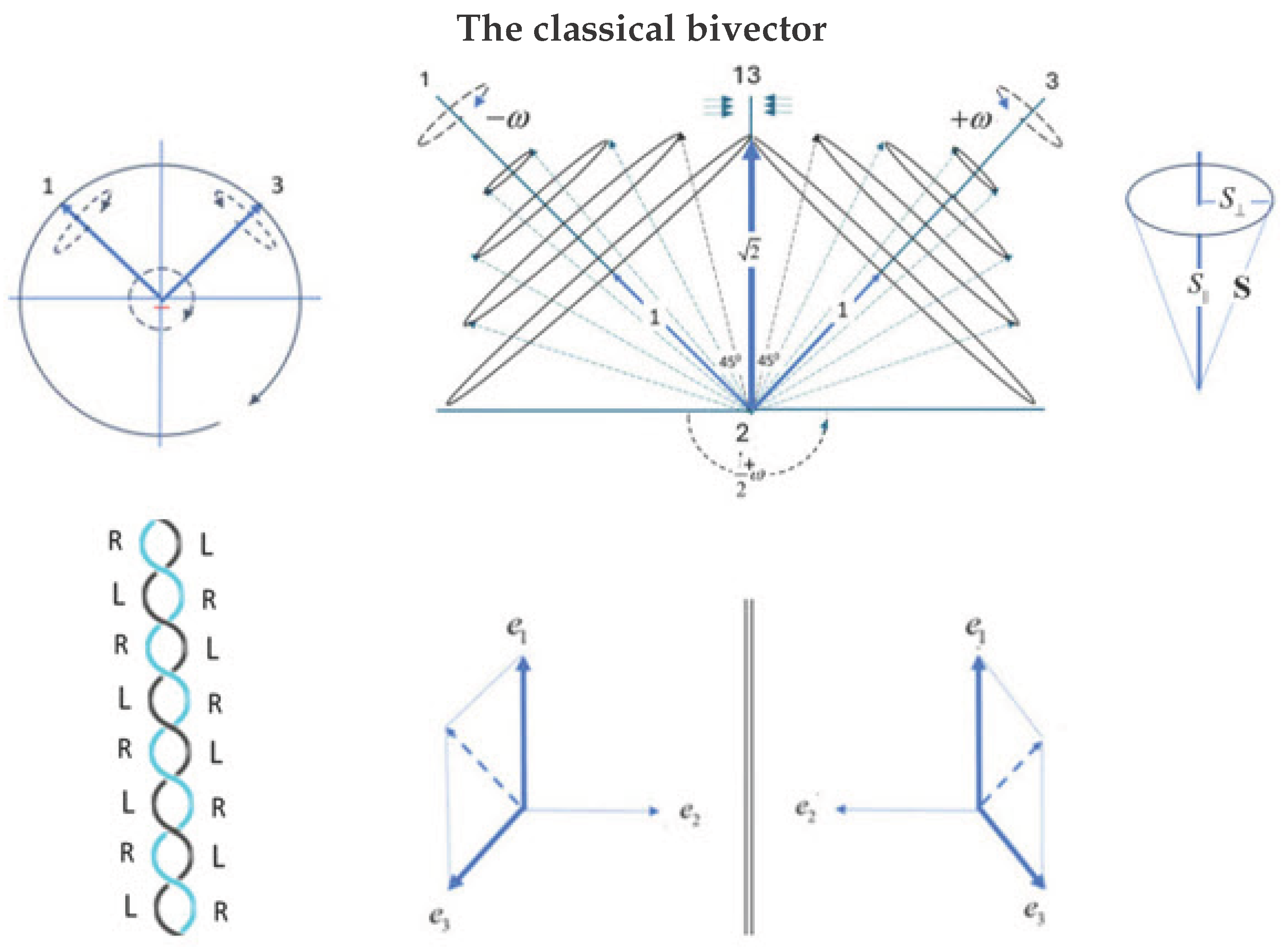
Figure 2.
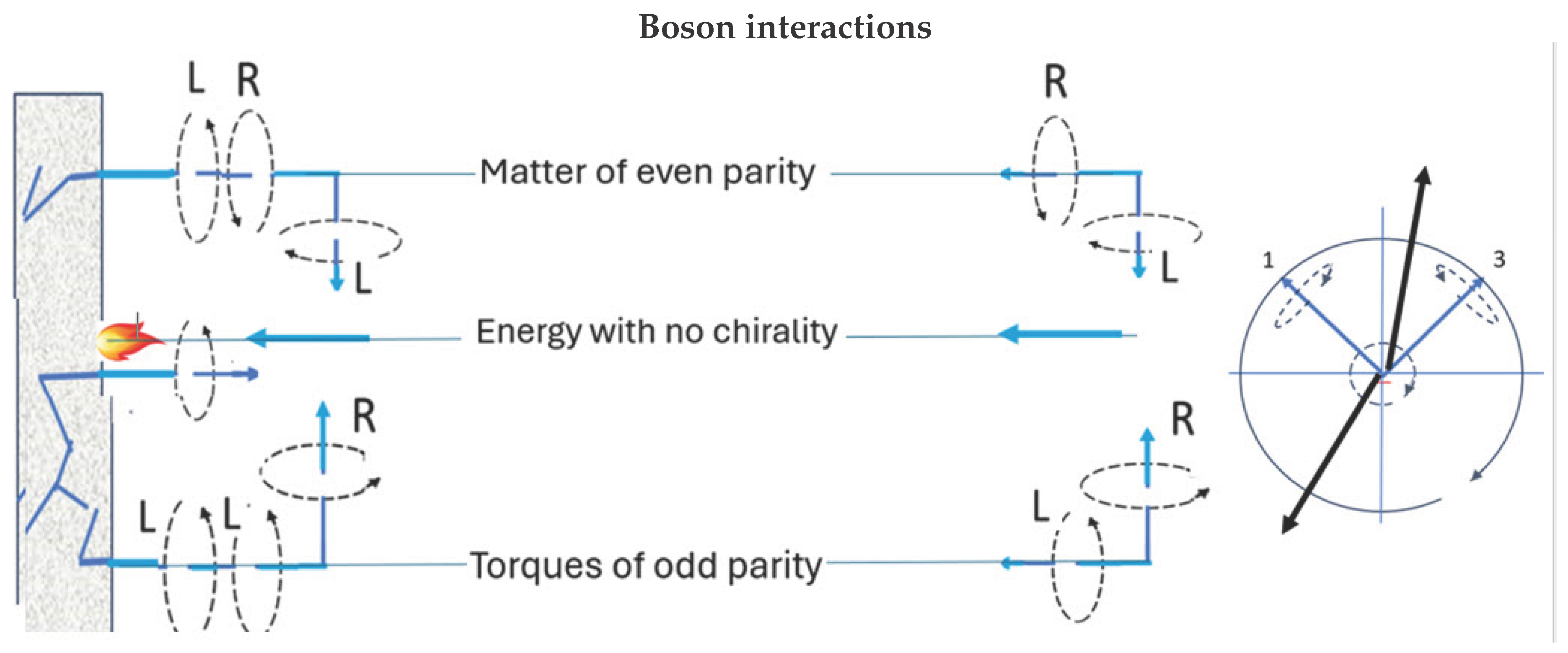
Three manifestations of bosons: When the incoming boson and the target have opposite chirality, they meld into matter of even parity. When their chiralities are equal, they combine to create a greater torque of odd parity. These require the polarizing field be outside the 13 interaction plane.
If the polarizing field lands within the interaction plane, 31, then a massive quantum impinges on the surface with no chirality. The long arrows denote two positions of the polarizing field vector: one in the interaction plane and the other outside of it.
Figure 2.
Three manifestations of bosons: When the incoming boson and the target have opposite chirality, they meld into matter of even parity. When their chiralities are equal, they combine to create a greater torque of odd parity. These require the polarizing field be outside the 13 interaction plane.
If the polarizing field lands within the interaction plane, 31, then a massive quantum impinges on the surface with no chirality. The long arrows denote two positions of the polarizing field vector: one in the interaction plane and the other outside of it.
Disclaimer/Publisher’s Note: The statements, opinions and data contained in all publications are solely those of the individual author(s) and contributor(s) and not of MDPI and/or the editor(s). MDPI and/or the editor(s) disclaim responsibility for any injury to people or property resulting from any ideas, methods, instructions or products referred to in the content. |
© 2025 by the authors. Licensee MDPI, Basel, Switzerland. This article is an open access article distributed under the terms and conditions of the Creative Commons Attribution (CC BY) license (http://creativecommons.org/licenses/by/4.0/).
Copyright: This open access article is published under a Creative Commons CC BY 4.0 license, which permit the free download, distribution, and reuse, provided that the author and preprint are cited in any reuse.


