1. Introduction
According to the general principles of (local) quantum field theory (QFT) [
1], observables in a spacelike region (i.e. in Euclidean space) can have singularities only for negative values of their argument
. However, for large
values, these observables are usually represented as power expansions in the running coupling constant (couplant)
, which has a ghostly singularity, the so-called Landau pole, at
. Therefore, to restore the analyticity of the considered expansions, this pole in the strong couplant should be removed.
The strong couplant
obeys the renormalization group equation
with some boundary condition and the QCD
-function:
where
for
f active quark flavors. Really now the first fifth coefficients, i.e.
with
, are exactly known [
2,
3,
4]. In our present consideration we will need only
.
Note that in Eq. (
2) we have added the first coefficient of the QCD
-function to the
definition, as is usually done in the case of analytic couplants (see, e.g., Refs. [
5,
6,
7,
8,
9]).
So, at the leading order (LO), at the next-to-leading order (NLO) and the next-to-next-to-leading order (NNLO), where
,
and
, respectively, we have from Eq. (
1)
i.e.
contain poles and other singularities at
.
In a timelike region (
) (i.e., in Minkowski space), the definition of a running couplant turns out to be quite difficult. The reason for the problem is that, strictly speaking, the expansion of perturbation theory (PT) in QCD cannot be defined directly in this region. Since the early days of QCD, much effort has been made to determine the appropriate Minkowski coupling parameter needed to describe important timelike processes such as,
-annihilation into hadrons, quarkonia and
-lepton decays into hadrons. Most of the attempts (see, for example, [
10]) have been based on the analytical continuation of strong couplant from the deep Euclidean region, where perturbative QCD calculations can be performed, to the Minkowski space, where physical measurements are made. In other developments, analytical expressions for a LO couplant were obtained [
11] directly in Minkowski space, using an integral transformation from the spacelike to the timelike mode from the Adler D-function.
In Refs. [
5,
6] an efficient approach was developed to eliminate the Landau singularity without introducing extraneous infrared controllers, such as the gluon effective mass (see, e.g., [
12]).
1 This method is based on a dispersion relation that relates the new analytic couplant
to the spectral function
obtained in the PT framework. In LO this gives
The [
5,
6] approach follows the corresponding results [
14] obtained in the framework of Quantum Electrodynamics. Similarly, the analytical images of a running coupling in the Minkowski space are defined using another linear operation
So, we repeat once again: the spectral function in the dispersion relations (
5) and (
6) is taken directly from PT, and the analytical couplants
and
are restored using the corresponding dispersion relations. This approach is usually called the
Minimal Approach (MA) (see, e.g., [
15]) or the
Analytical Perturbation Theory (APT) [
5,
6].
2
Thus, MA QCD is a very convenient approach that combines the analytical properties of QFT quantities and the results obtained in the framework of perturbative QCD, leading to the appearance of the MA couplants and , which are close to the usual strong couplant in the limit of large values and completely different from for small values, i.e. for .
A further APT development is the so-called fractional APT (FAPT) [
7,
8,
9], which extends the construction principles described above to PT series, starting from non-integer powers of the couplant. In the framework of QFT, such series arise for quantities that have non-zero anomalous dimensions. Compact expressions for quantities within the FAPT framework were obtained mainly in LO, but this approach was also used in higher orders, mainly by re-expanding the corresponding couplants in powers of the LO couplant, as well as using some approximations.
In this review, we show the main properties of MA couplants in the FAPT framework, obtained in Refs. [
18,
19] using the so-called
-expansion. Note that for an ordinary couplant, this expansion is applicable only for large
values, i.e. for
. However, as shown in [
18,
19], the situation is quite different in the case of analytic couplants, and this
-expansion is applicable for all values of the argument. This is due to the fact that the non-leading expansion corrections vanish not only at
, but also at
,
3 which leads only to nonzero (small) corrections in the region
.
Below we consider the representations for the MA couplants and their (fractional) derivatives obtained in [
18,
19] (see also [
20]) and valid in principle in any PT order. However, in order to avoid cumbersome formulas, but at the same time to show the main features of the approach obtained in [
18,
19], we confine ourselves to considering only the first three PT orders.
Moreover, in this review, we show FAPT applications for the Higgs-boson decay into a bottom-antibottom pair and the description of the polarized Bjorken sum rule (BSR). The results shown here have been recently obtained in Refs. [
19] and Refs. [
21,
22], respetively. In contrast to the formulas, the results for the Higgs boson decay and the polarized Bjorken sum rule will be shown in the first five PT orders, as was obtained in [
19,
21,
22].
The paper is organized as follows. In
Section 2 we firstly review the basic properties of the usual strong couplant and its
-expansion.
Section 3 contains fractional derivatives (i.e.
-derivatives) of the usual strong couplant, which
-expansions can be represented as some operators acting on the
-derivatives of the LO strong couplant. In Sections 4 and 5 we present the results for the MA couplands.
Section 6 contains formulas conveninet for
. In Sections 7 and 8 we present the integrals repsenentations for the MA couplands. Sections 9 and 10 contain applications of this approach to the Higgs-boson decay into a bottom-antibottom pair and the Bjorken sum rule, respectively. In conclusion, some final discussions are given. In addition, we have several Appendices, which contain most complicated expressions.
3. Fractional Derivatives
Following [
30,
31], we introduce the derivatives (in the
-order of of PT)
which are very convenient in the case of the analytical QCD (see, e.g., [
32]).
The series of derivatives can successfully replace the corresponding series of -degrees. Indeed, each the derivative reduces the degree, but is accompanied by an additional -function . Thus, each application of a derivative yields an additional , and thus indeed possible to use series of derivatives instead of series of -powers.
In LO, the series of derivatives
are exactly the same as
. Beyond LO, the relationship between
and
was established in [
31,
33] and extended to fractional cases, where
is a non-integer
, in Ref. [
34].
Now consider the
-expansion of
. We can raise the
-power of the results (
7) and (
9) and then restore
using the relations between
and
obtained in [
34] (see Appendix A) This operation is carried out in more details in Appendix B to [
18] (see also Appendix A to [
20]). Here we present only the final results, which have the form
7:
where
and
are combinations of the Euler
-functions and their derivatives.
The representation (
13) of the
corrections as
-operators is very important
8 and allows us to similarly present high-order results for the (
-expansion) of analytic couplants.
9. Decay
In Ref. [
18] we used the polarized Bjorken sum rule [
62] as an example for the application of the MA couplant
, which is a popular object of study in the framework of analytic QCD (see [
38,
40,
60,
61]). Here we consider the decay of the Higgs boson into a bottom-antibottom pair, which is also a popular application of the MA couplant
(see, e.g., [
8] and reviews in Ref. [
16]).
The Higgs-boson decay into a bottom-antibottom pair can be expressed in QCD by means of the correlator
of two quark scalar (S) currents in terms of the discontinuity of its imaginary part, i.e.,
, so that the width reads
Direct multi-loop calculations were performed in the Euclidean (spacelike) domain for the corresponding Adler function
(see Refs. [
41,
42,
43,
44]). Hence, we write (
and
because the additional factor
)
where for
the coefficients
are
Taking the imagine part, one has
and for
[
43,
45]
Here
has the form (see Appendix C):
where
and
are done in Eq. (
A32). For
we have
The normalization constant
cab be obtained as (see, e.g., [
16])
since
GeV.
We can express all results through derivatives
(see Appendix A):
where
where
are given in Appendix A.
For
and
, we have
Performing the same analysis for the Adler function we have
where
We express all results through derivatives
:
where
For
and
, we have
As it was discussed earlier in [
8] in FAPT there are the following representation for
The results for
are shown in
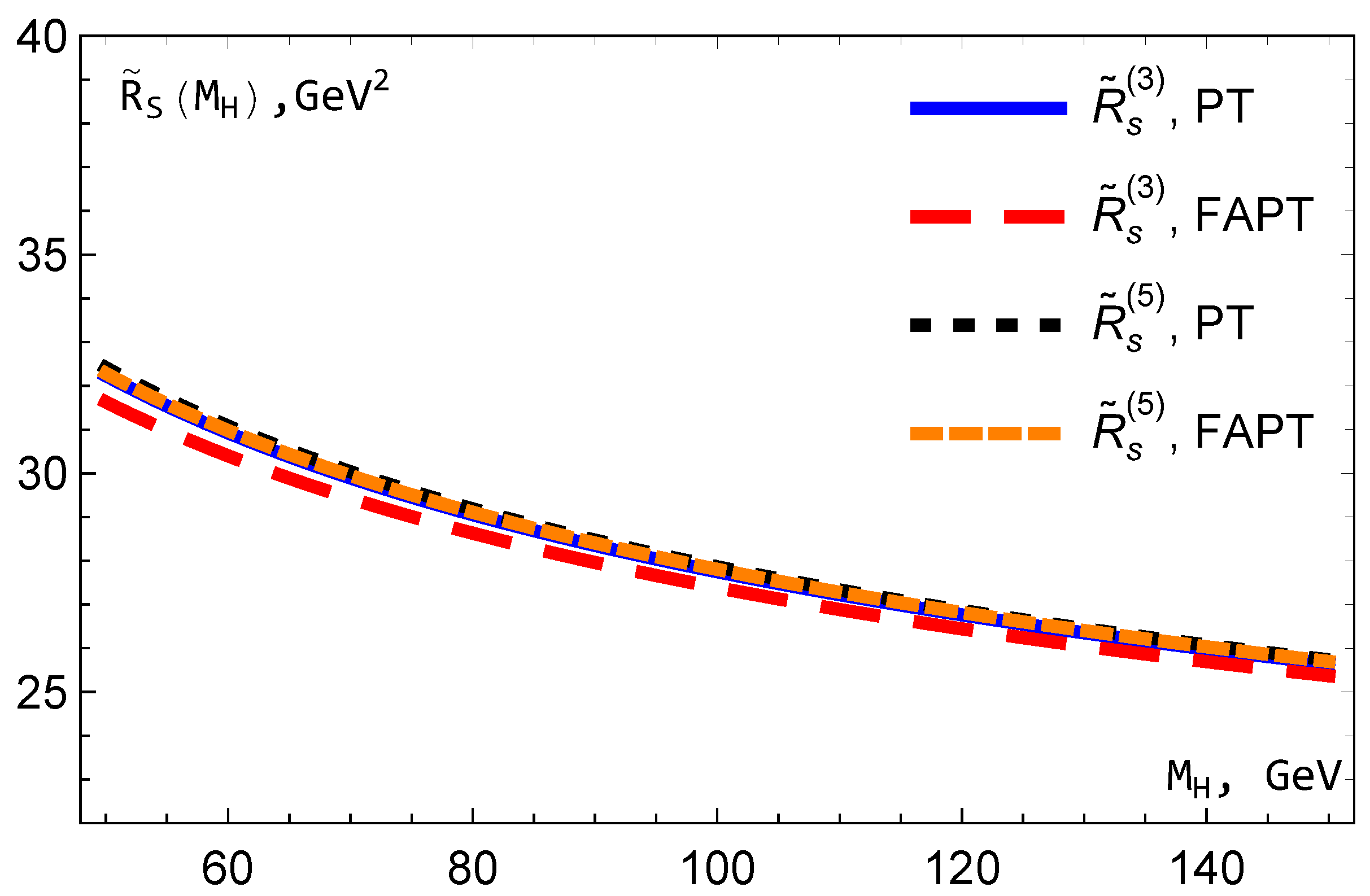
Figure 14. We see that the FAPT results (
99) are lower than those (
90) based on the conventional PT. This is in full agreement with arguments given in [
16]. But the difference becomes less notable as the PT order increases. Indeed, for N
3LO the difference is very small, which proves the assumption about the possibility of using
expression for
with
, which was done in Ref. [
8].
The results for
in the N
mLO approximation using
from Eqs. (
87) and (
90) are exactly same and have the following form:
The corresponding results for
with
form Eq. (
99) are very similar to ones in (
100). They are:
So, we see a good agreement between the results obtained in FAPT and in the framework of the usual PT.
It is clearly seen that the results of FAPT are very also close to the results [
46] obtained in the framework of the now very popular Principle of Maximum Conformality [
47] (for the recent review, see [
48]). Indeed, our results are within the band obtained by varying the renormalization scale.
The Standard Model expectation is [
49]
The ratios of the measured events yield to the Standard Model expectations are
[
50] in ATLAS Collaboration and
[
51] in SMC Collaboration (see also [
52]).
Thus, our results obtained in both approaches, in the standard perturbation theory and in analytical QCD, are in good agreement both with the Standard Model expectations [
49] and with the experimental data [
50,
51].
10. Bjorken Sum Rule
The polarized BSR [
53] (see also [
54,
55]) is defined as the difference between the proton and neutron polarized SFs, integrated over the entire interval
x
Theoretically, the quantity can be written in the OPE form (see Ref. [
56,
57])
where
=1.2762 ± 0.0005 [
24] is the nucleon axial charge,
is the leading-twist (or twist-two) contribution, and
are the higher-twist (HT) contributions.
9
Since we plan to consider in particular very small
values here, the representation (
104) of the HT a number of infinite terms. To avoid that, it is preferable to use the so-called "massive" twist-four representation, which includes a part of the HT contributions of (
104) (see Refs. [
58,
59]):
10
where the values of
and
have been fitted in Refs. [
60,
61] in the different analytic QCD models.
In the case of MA QCD, from [
61] one can see that in (
105)
where the statistical (small) and systematic (large) uncertainties are presented.
Up to the
k-th PT order, the twist-two part has the form
where
,
and
are known from exact calculations (see, for example, [
62]). The exact
value is not known, but it was estimated in Ref. [
63].
Converting the couplant powers into its derivatives, we have
where
and
.
In MA QCD, the results (
105) become as follows (some analyses based on other approaches can be found in [
64,
65,
66])
where the perturbative part
takes the same form, however, with analytic couplant
(the corresponding expressions are taken from [
18])
We would like to note the coefficients
depend on the number
f of active quarks, which changes at thresholds
, where some additional quark comes to play at
. Here
is the
mass of
f quark. So, the coupling constant
is
f-dependent and the
f-dependence can be taken into the corresponding QCD parameter
. , i.e.
contribute to above Eqs. (
107), (
108) and (
111).
The relations between
and
are coming from the decoupling relations, i.e. the relations between
and
. In the
scheme, the decoupling relations are known up to four-loop order [
25] and they are usually used at
, where the relations are simplified (for a recent review, see e.g. [
67]).
Here we will not consider the f-dependence of and . Since we will mainly consider the region of low , we will use the results for , which we need to construct the analytic couplant for small values.
For the
k-th order of PT, we use the results (
11) for
taken from the recent Ref. [
27], which corresponds to the middle value of the world average
[
24]. We use also
, since in highest orders
values become very similar. Moreover, since the results for
and for
are taken from the range of
values where the difference between the analytic and usual couplants is small, we use the values (
11) also in the case of anaytic QCD.
For the case of 3 active quark flavors (
), which is accepted in this paper, we have
i.e., the coefficients in the series of derivatives are slightly smaller.
10.1. Results
The fitting results of experimental data (see [
68,
69,
70,
71,
72,
73,
74]) obtained only with statistical uncertainties are presented in
Table 1 and shown in
Figure 15 and
Figure 16. For the fits we use
-independent
and
and the two-twist part shown in Eqs. (
108), (
111) for regular PT and APT, respectively.
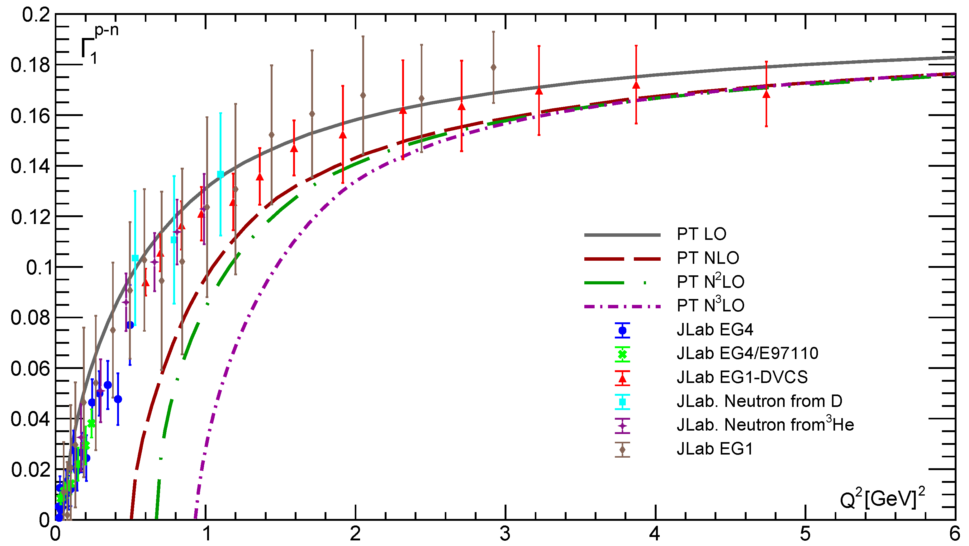
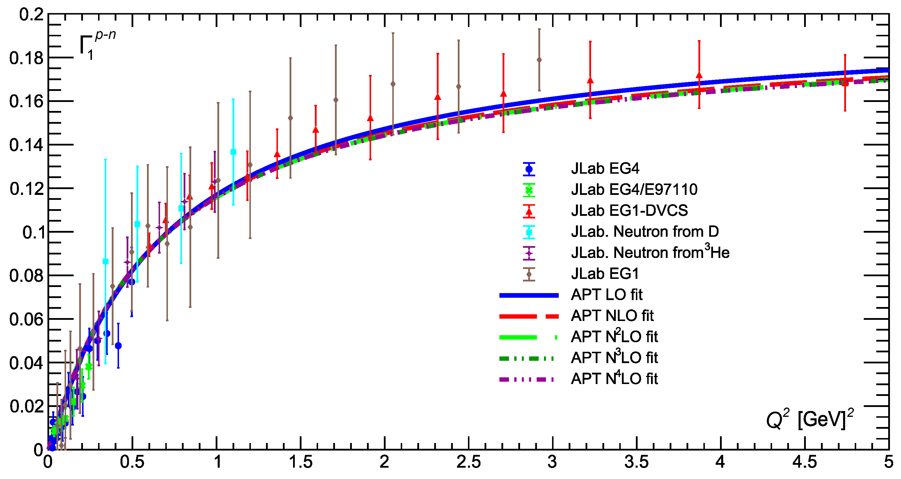
As it can be seen in
Figure 15, with the exception of LO, the results obtained using conventional couplant are very poor. Moreover, the discrepancy in this case increases with the order of PT (see also [
38,
39,
60,
61] for similar analyses). The LO results describe experimental points relatively well, since the value of
is quite small compared to other
, and disagreement with the data begins at lower values of
(see
Figure 4 below). Thus, using the “massive” twist-four form (
105) does not improve these results, since with
conventional couplants become singular, which leads to large and negative results for the twist-two part (
107). So, as the PT order increases, ordinary couplants become singular for ever larger
values, while BSR tends to negative values for ever larger
values.
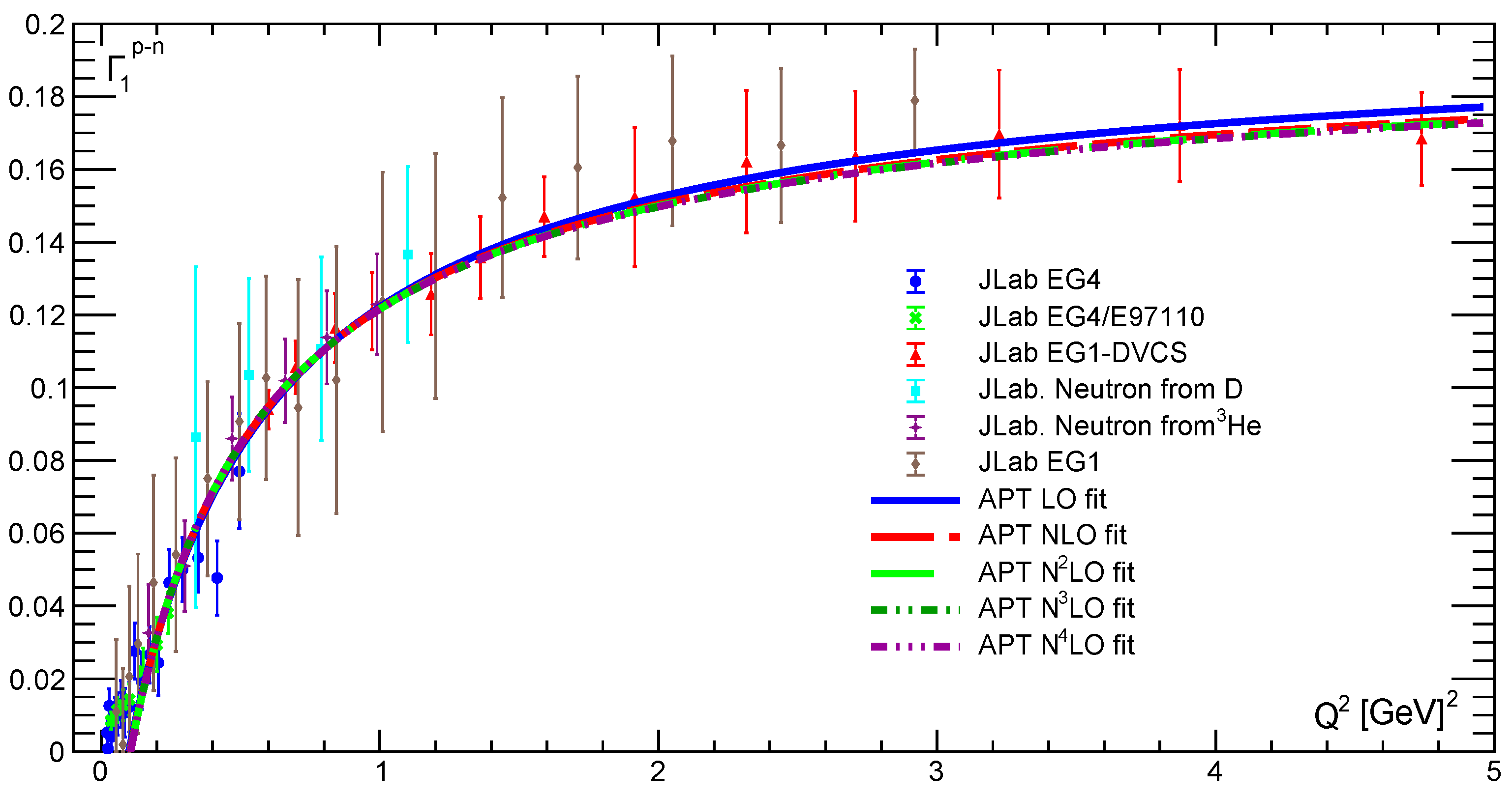
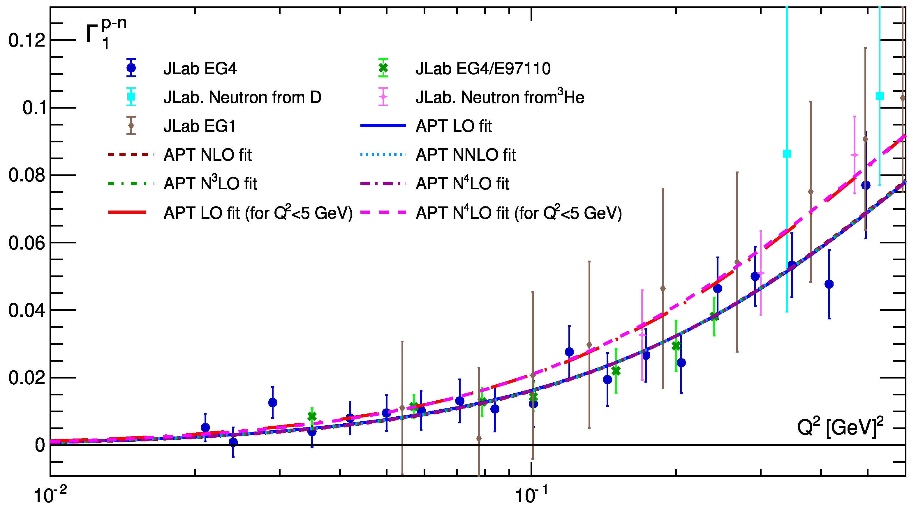
In contrast, our results obtained for different APT orders are practically equivalent: the corresponding curves become indistinguishable when
approaches 0 and slightly different everywhere else. As can be seen in
Figure 16, the fit quality is pretty high, which is demonstrated by the values of the corresponding
(see
Table 1).
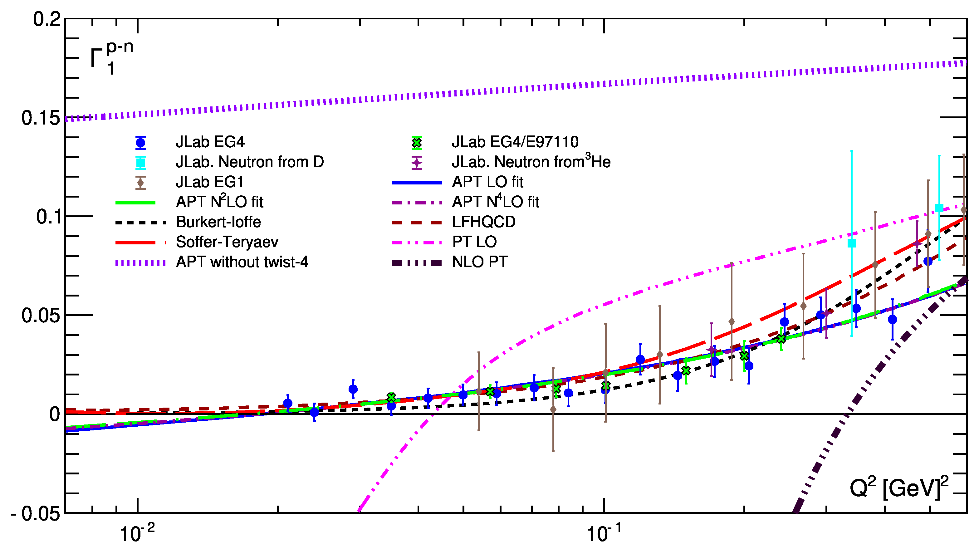
10.2. Low Values
The full picture, however, is more complex than shown in
Figure 16. The APT fitting curves become negative (see
Figure 17) when we move to very low values of
:
0.1 GeV
2. So, the good quality of the fits shown in
Table 1 was obtained due to good agreement with experimenatl data at
0.2 GeV
2. The picture improves significantly when we compare our result with experimental data for
0.6 GeV
2 (see
Figure 18 and Ref. [
21]).
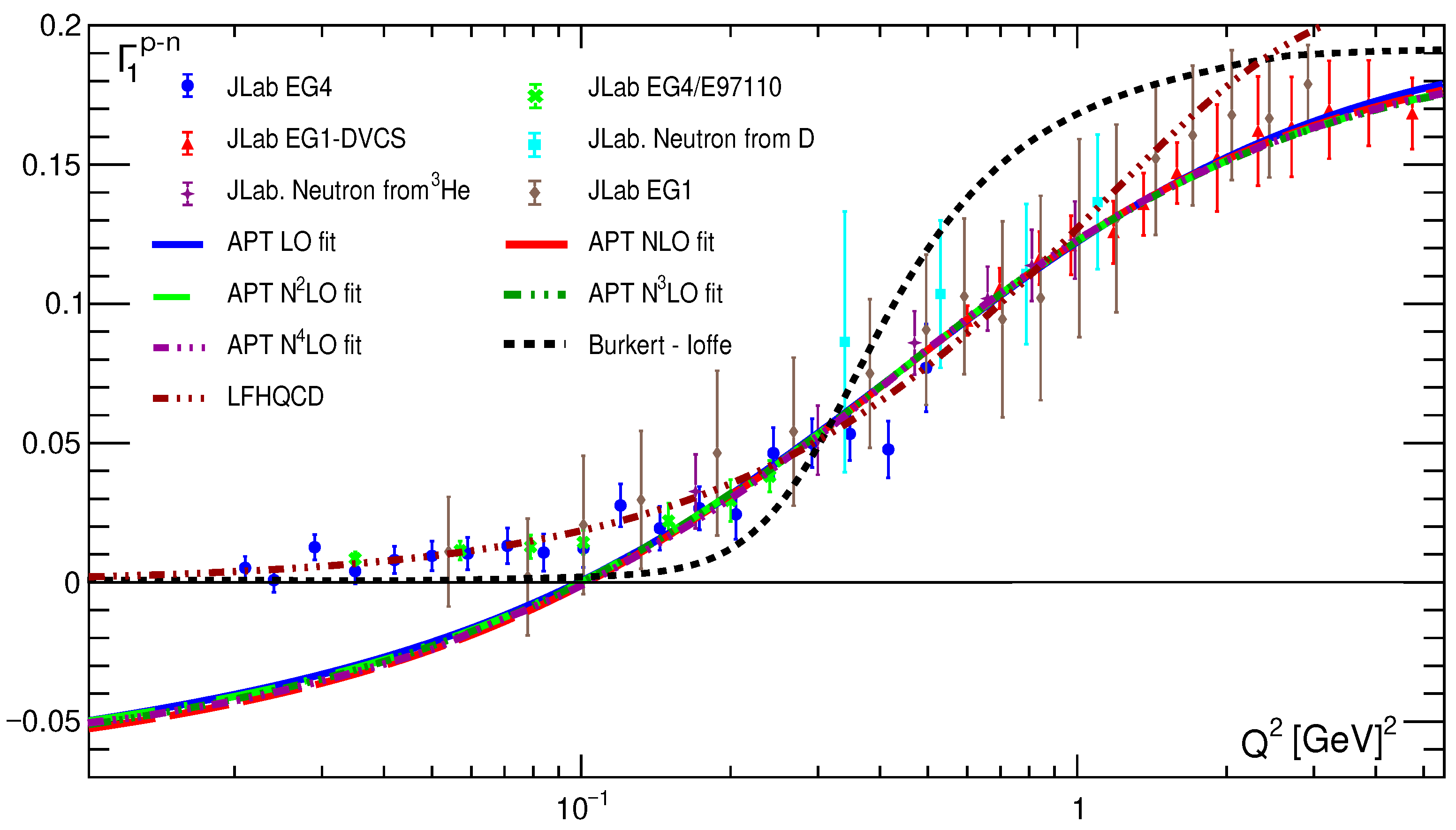
Figure 18 also shows contributions from conventional PT in the first two orders: the LO and NLO predictions have nothing in common with experimental data. As we mentioned above, higher orders lead to even worse agreement, and they are not shown. The purple curve emphasizes the key role of the twist-four contribution (see also [
39,
75]) and the discussions therein). Excluding this contribution, the value of
is about 0.16, which is very far from the experimental data.
At
GeV
2, we also see the good agreement with the phenomenological models: LFHQCD [
76] and the correct IR limit of Burkert–Ioffe model [
77].For larger values of
, our results are lower than the results of phenomenological models, and for
GeV
2 below the experimental data.
Nevertheless, even in this case where very good agreement with experimental data with 0.6 GeV2 is demonstrated, our results for take negative unphysical values when 0.02 GeV2. The reason for this phenomenon can be shown by considering photoproduction within APT, which is the topic of the next subsection.
10.3. Photoproduction
To understand the problem
, demonstrated above, we consider the photoproduction case. In the
k-th order of MA QCD
and, so, we have
The finitness of cross-section in the real photon limit leads to [
58]
For
, we have
shown in (
106) and in
Table 1.
So, as can be seen from
Table 1, the finiteness of the cross section in the real photon limit is violated in our approaches.
11 This violation leads to negative values of
. Note that this violation is less for experimental data sets with
GeV
2, where the obtained values for
are essentially less then those obtained in the case of experimental data with
GeV
2. Smaller values of
lead to negative values of
, when
GeV
2 (see
Figure 4).
10.4. Gerasimov-Drell-Hearn and Burkhardt-Cottingham Sum Rules
Now we plan to improve this analysis by involving the result (
110) at low
values and also taking into account the “massive” twist-six term, similar to the twist-four shown in Eq. (
105).
Moreover, we take into account also the GDH and BC sum rules, which lead to (see [
58,
59,
78,
79])
where
and
are proton and neutron magnetic moments, respectively, and
= 0.938 GeV is a nucleon mass. Note that the value of
G is small.
In agreement with the definition (
12), we have that
Then, for
we obtain at any
n value, that
but very slowly, that the derivative
Thus, after application the derivative
for
, every term in
becomes to be divergent at
. To produce finitness at
for the l.h.s. of (
117), we can assume the relation between twist-two and twist-four terms, that leads to the appearance of a new contribution
which can be done to be regular at
.
The form (
121) suggests the following idea about a modification of
in (
110):
where we added the “massive” twist-six term and introduced different masses in both higher-twist terms and into the modification factor
.
The finitness of cross-section in the real photon limit leads now to [
58]
and, thus, we have
From Eq. (
122) and condition (
117), we obtain
where
(see Eq. (
114)).
Using
(i.e.
), we have
Taking the results (
123) and (
126) together, we have at the end the following results:
Since the value of G is small, so and .
The fitting results of theoretical predictions based on Eq. (
122) with
and
done in (
127), are presented in
Table 2 and on
Figure 19 and
Figure 20.
As one can see in
Table 2, the obtained results for
are different if we take the full data set and the limited one with
0.6 GeV
2. However, the difference is significantly less than it was in
Table 1. Moreover, the results obtained in the fits using the full data set and shown in
Table 1 and
Table 2 are quite similar, too.
Figure 20 also shows that the results of fitting the full set of experimental data are in better agreement with the data at
GeV
2, as it should be, since these data are involved in the analyses of the full set of experimental data.
The results shown in
Table 1 and
Table 2 are not changes practically when heavy quark contributions [
80] were added in consideration (see [
81]).
11. Conclusions
In this paper we presented an overview of fractional analytic QCD and its application for Higgs-boson decay into a bottom-antibottom pair and for the polarized Bjorken sum rule.
We have considered
-expansions of
-derivatives of the strong couplant
expressed as combinations of operators
(
14) applied to the LO couplant
. Applying the same operators to the
-derivatives of the LO MA couplant
, we obtained four different representations for the
-derivatives of the MA couplants, i.e.
, in each
i-order of perturbation theory: one form contains a combination of Polylogariths; the other contains an expansion of the generalized Euler
-function, and the third is based on dispersion integrals containing the LO spectral function. We also obtained a fourth representation based on the dispersion integral containing the
i-order spectral function. All results are presented up to the 5th order of perturbation theory, where the corresponding coefficients of the QCD
-function are well known (see [
2,
3]).
The high-order corrections are negligible in the
and
asymptotics and are nonzero in the vicinity of the point
. Thus, in fact, they are really only small corrections to the LO MA couplant
. This proves the possibility of expansions of high-order couplants
via the LO couplants
, which was done in Ref. [
9], as well as the possibility of various approximations used in [
28,
38,
39,
40].
As can be clearly seen, all our results (
up to the 5th order of perturbation theory) have a compact form and do not contain complicated special functions, such as the Lambert
W-function [
82], which already appears at the two-loop order as an exact solution to the usual couplant and which was used to evaluate MA couplants in [
83].
Applying the same operators to the
-derivatives of the LO MA couplant
, we obtained two different representations (see Eqs. (
29) and (
71)) for the
-derivatives of the MA couplants, i.e.
introduced for timelike processes, in each
i-order of perturbation theory: one form contains a combinations of trigonometric functions, and the other is based on dispersion integrals containing the
i-order spectral function. All results are presented up to the 5th order of perturbation theory, where the corresponding coefficients of the QCD
-function are well known (see [
2,
3]).
As in the case of
[
18] applied in the Euclidean space, high-order corrections for
are negligible in the
and
limits and are nonzero in the vicinity of the point
. Thus, in fact, there are actually only small corrections to the LO MA couplant
. In particular, this proves the possibility of expansions of high-order couplants
via the LO couplants
, which was done in Ref. [
9].
As an example, we examined the Higgs boson decay into a
pair and obtained results are in good agreement with the Standard Model expectations [
49] and with the experimental data [
50,
51]. Moreover, our results also in good agreement with studies based on the Principle Maximum Conformality [
47].
As a second application, we considered the Bjorken sum rule
in the framework of MA and perturbative QCD and obtained results similar to those obtained in previous studies [
21,
38,
39,
60,
61] for the first 4 orders of PT. The results based on the conventional PT do not agree with the experimental data. For some
values, the PT results become negative, since the high-order corrections are large and enter the twist-two term with a minus sign. APT in the minimal version leads to a good agreement with experimental data when we used the “massive” version (
110) for the twist-four contributions.
Examining low
behaviour, we found that there is a disagreement between the results obtained in the fits and application of MA QCD to photoproduction. The results of fits extented to low
lead to the negative values for Bjorken sum rule
:
that contrary to the finitness of cross-section in the real photon limit, which leads to
. Note that fits of experimental data at low
values (we used
0.6 GeV
2) lead to less magnitudes of negative values for
(see
Table 1 and
Table 2).
To solve the problem we considered low
modifications of OPE formula for
. Considering carefully one of them, Eq. (
122), we find good agreement with full sets of experimental data for Bjorken sum rule
and also with its
limit, i.e. with photoproduction. We see also good agreement with phenomenological modeles [
77,
78,
79], especially with LFHQCD [
76].
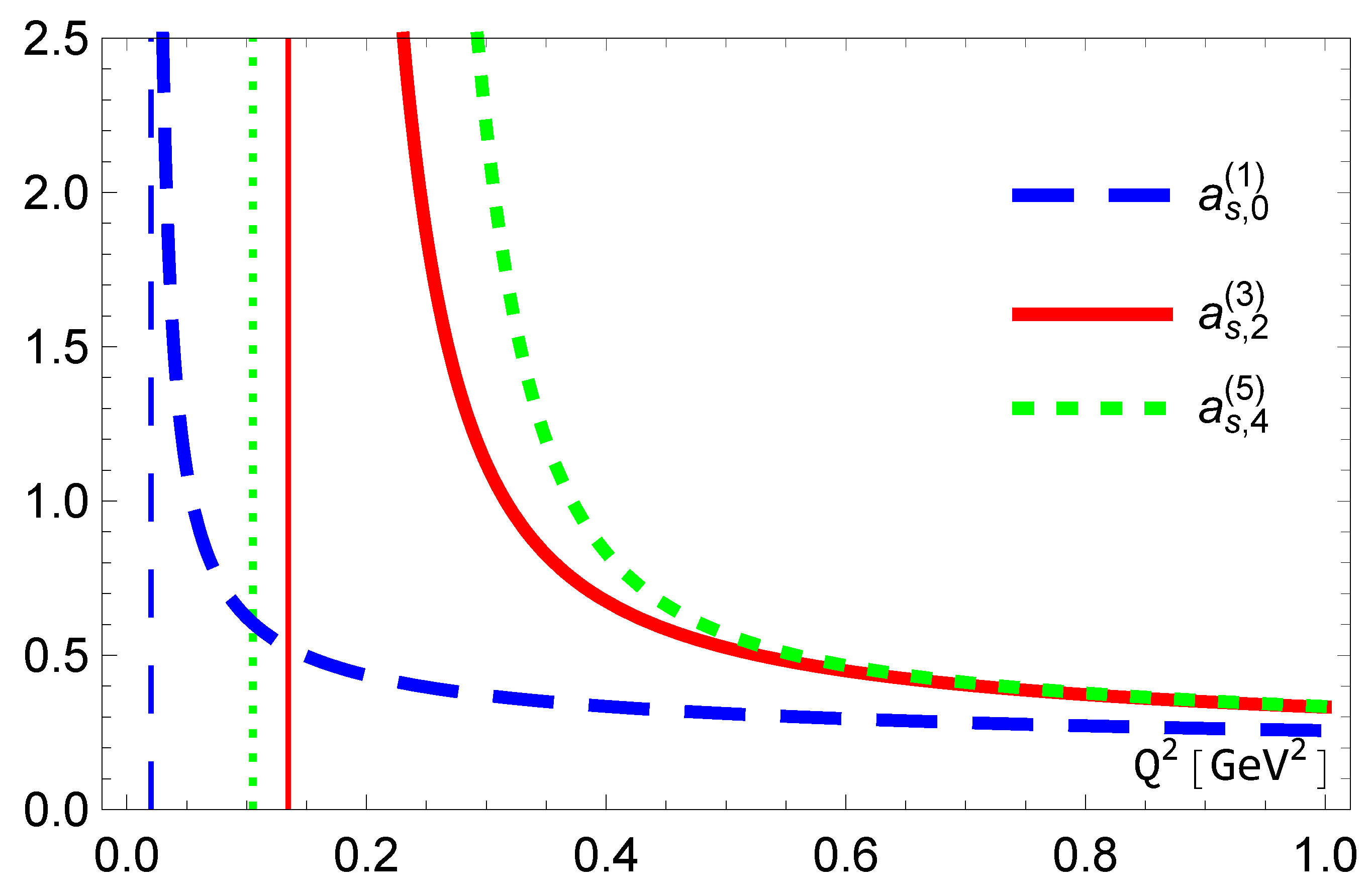
Figure 1.
The results for
and
(vertical lines) with
. Here and in the following figures, the
values shown in (
11) are used.
Figure 1.
The results for
and
(vertical lines) with
. Here and in the following figures, the
values shown in (
11) are used.
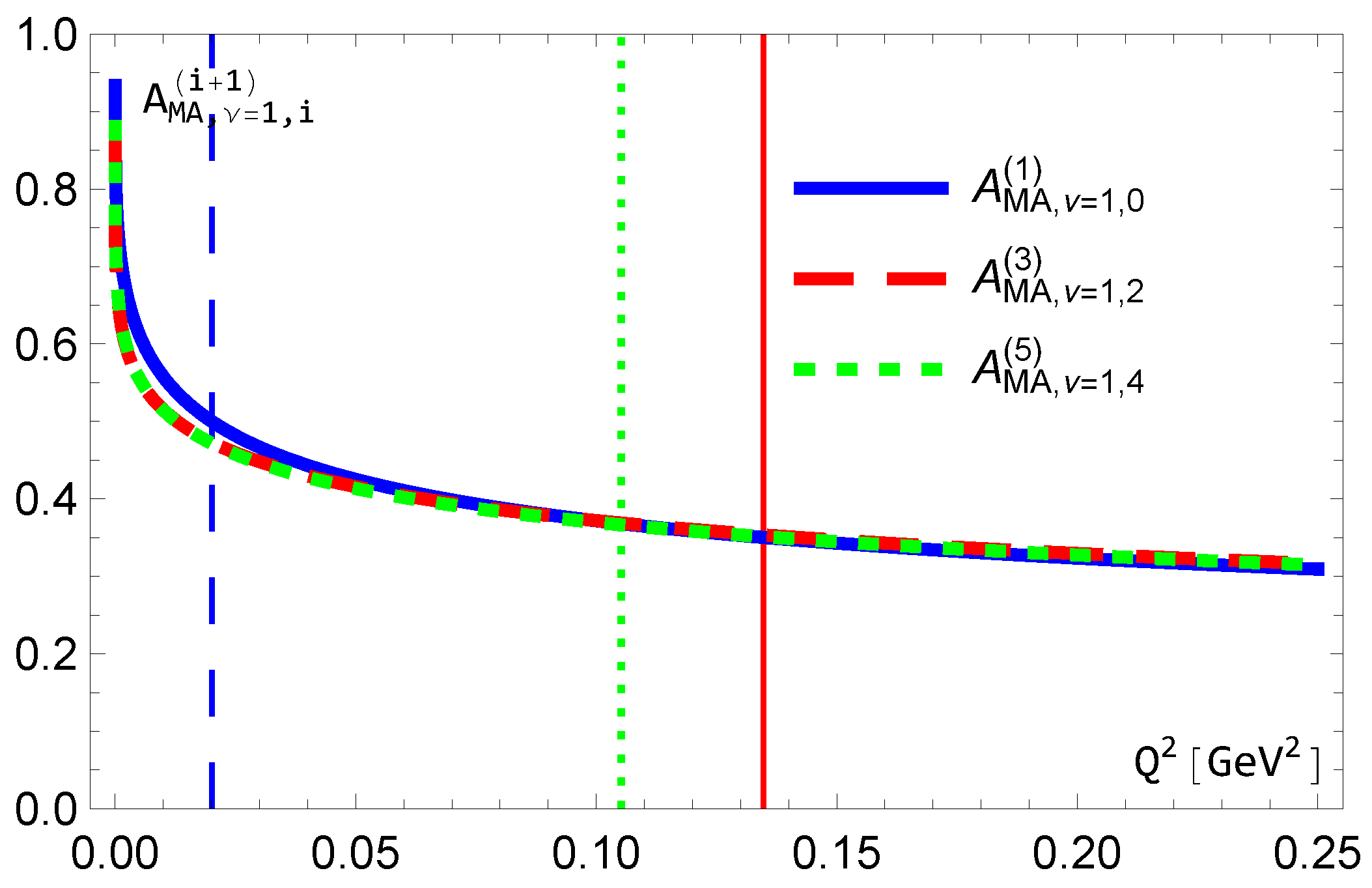
Figure 2.
The results for and (vertical lines) with .
Figure 2.
The results for and (vertical lines) with .
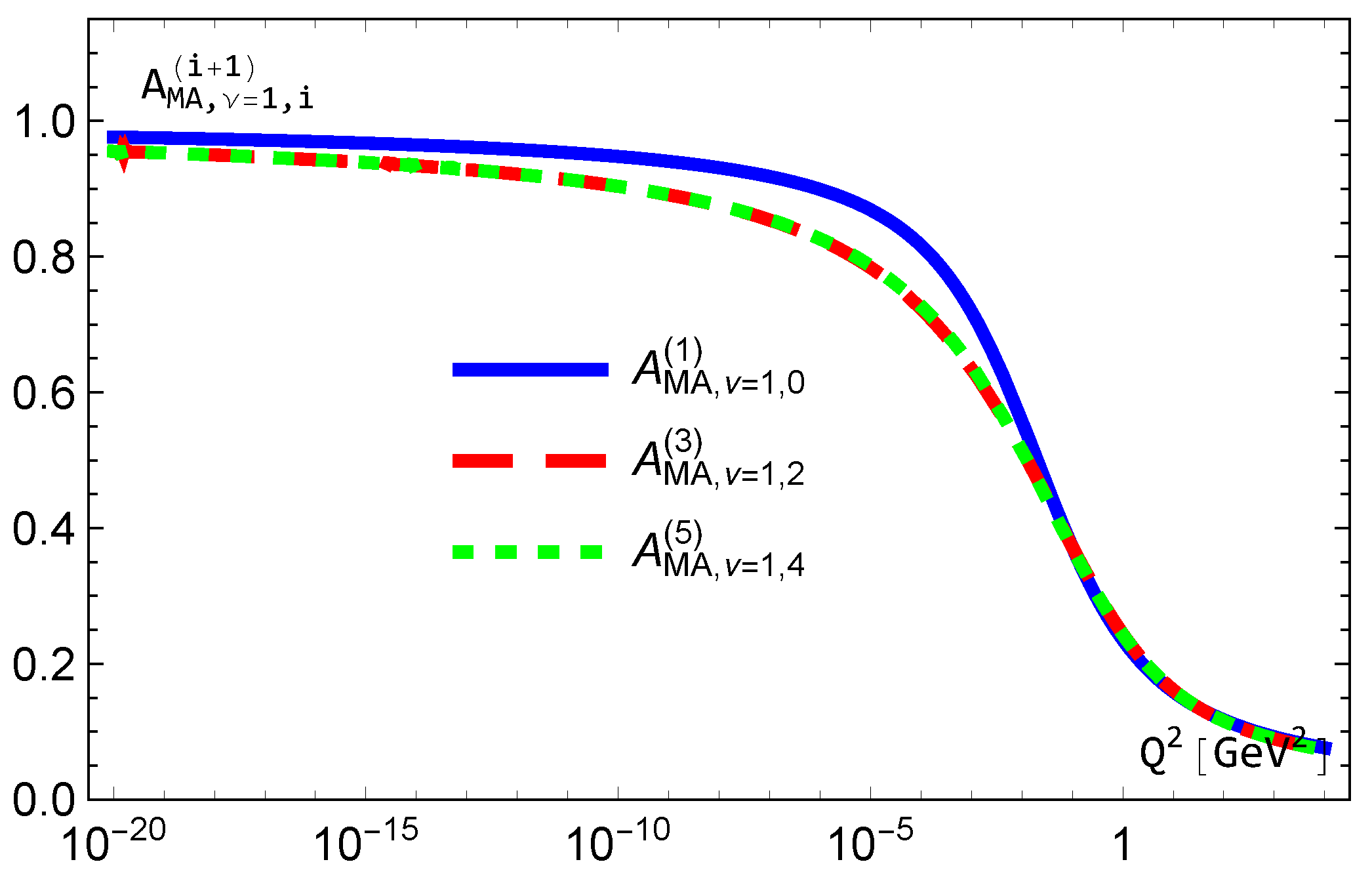
Figure 3.
The results for () but with the logarithmic scale.
Figure 3.
The results for () but with the logarithmic scale.
Figure 4.
The results for , and .
Figure 4.
The results for , and .
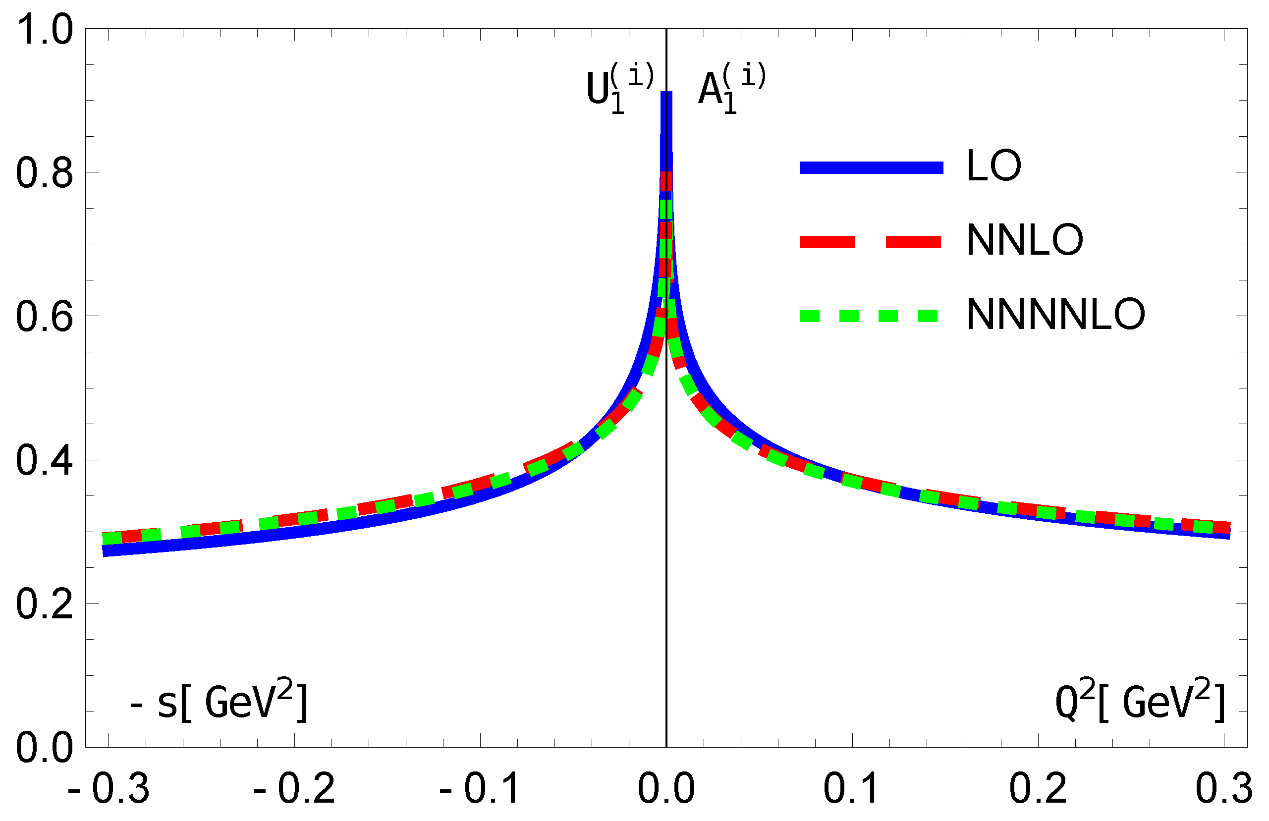
Figure 5.
The results for with .
Figure 5.
The results for with .
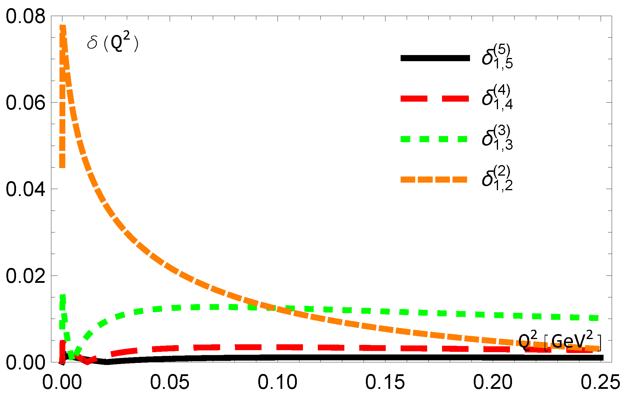
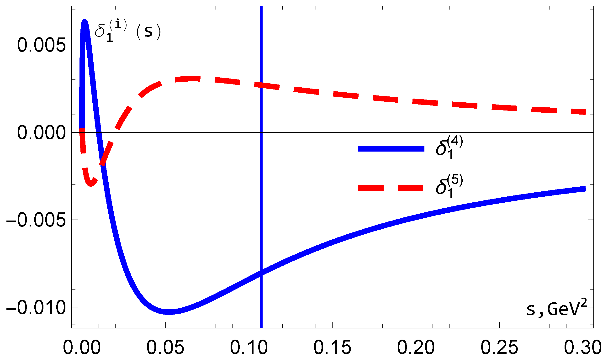
Figure 6.
1,3 and 5 orders of .The vertical lines indicate
Figure 6.
1,3 and 5 orders of .The vertical lines indicate
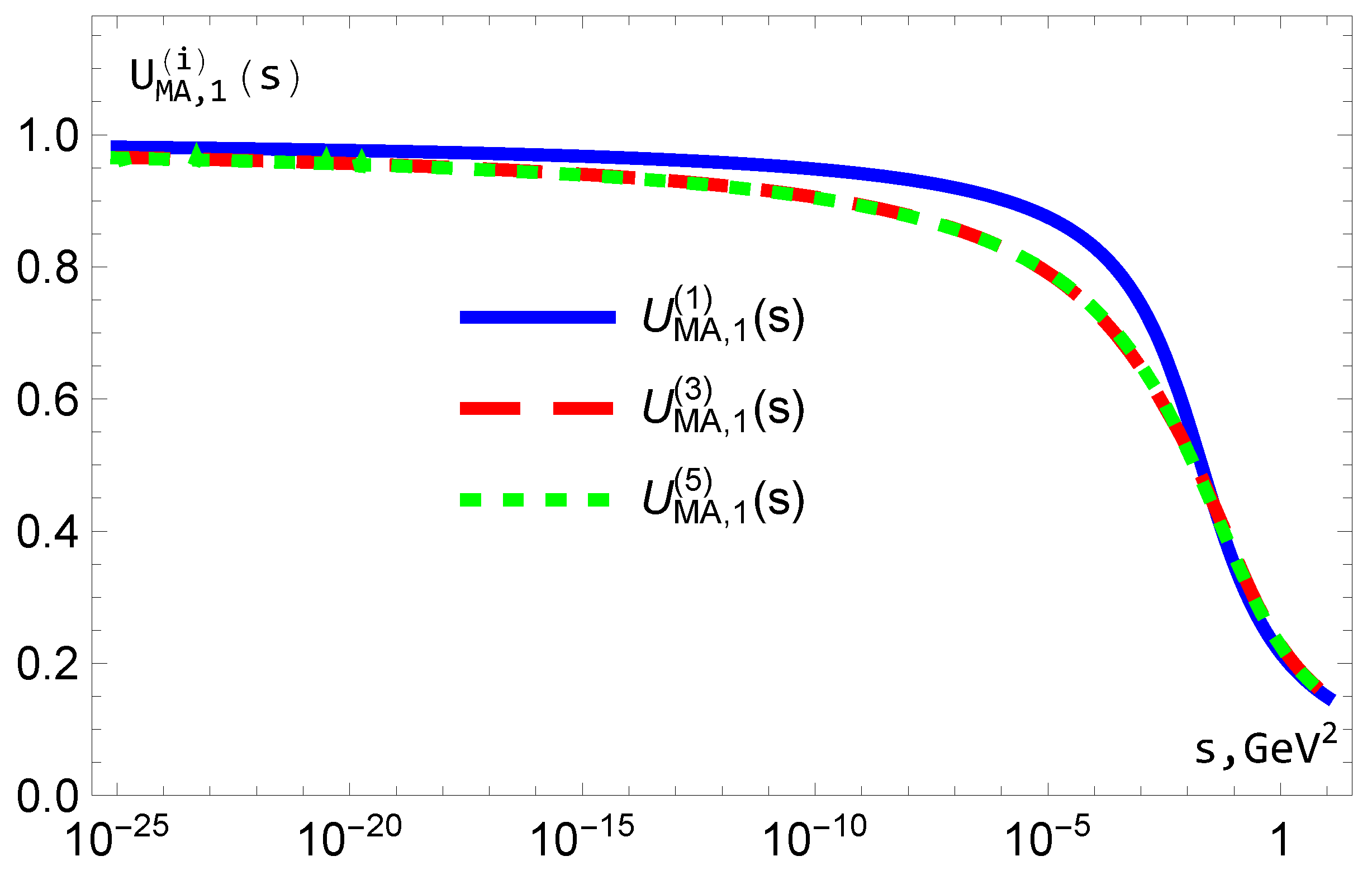
Figure 7.
1,3 and 5 orders of with logarithmic scale of s
Figure 7.
1,3 and 5 orders of with logarithmic scale of s
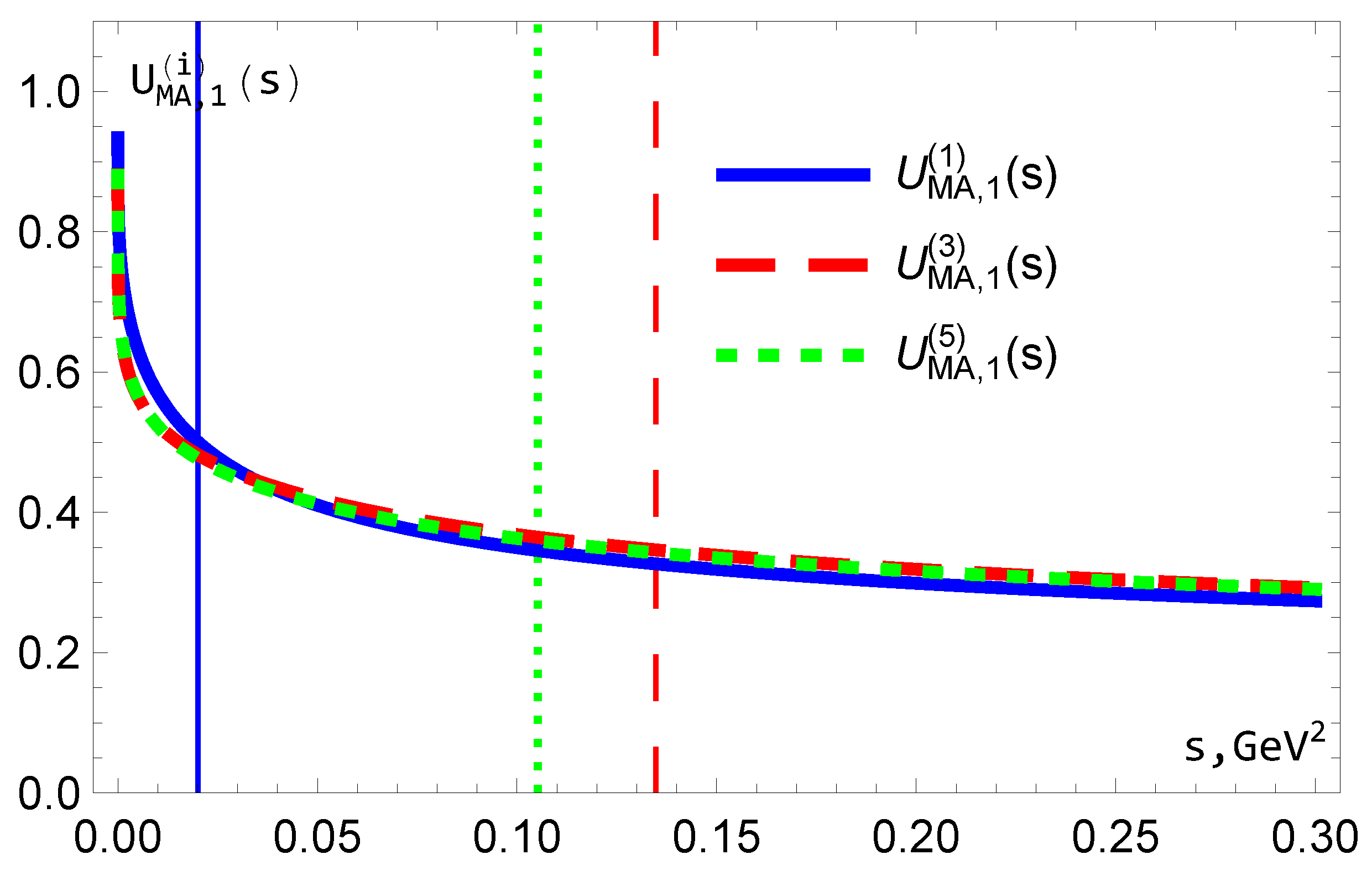
Figure 8.
with .The vertical lines indicate
Figure 8.
with .The vertical lines indicate
Figure 9.
with . The vertical line indicates
Figure 9.
with . The vertical line indicates
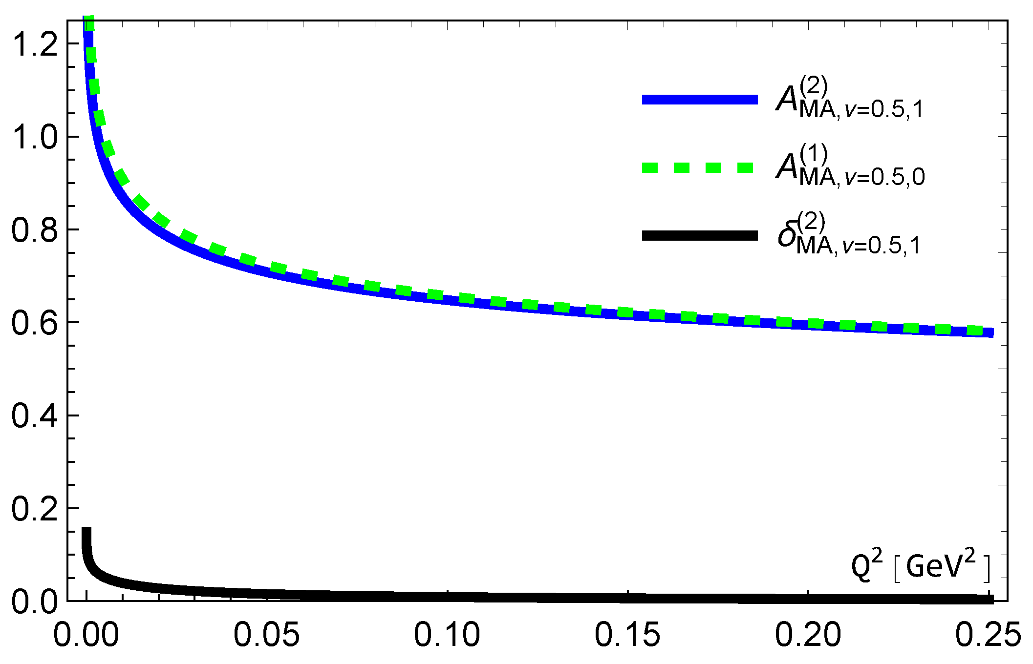
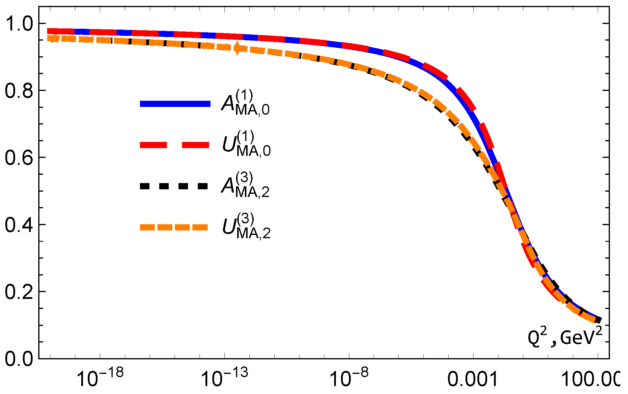
Figure 10.
The results for and with .
Figure 10.
The results for and with .
Figure 11.
1,3 and 5 orders of and
Figure 11.
1,3 and 5 orders of and
Figure 12.
1 and 2 orders of , and in Euclidean and Minkowki spaces.
Figure 12.
1 and 2 orders of , and in Euclidean and Minkowki spaces.
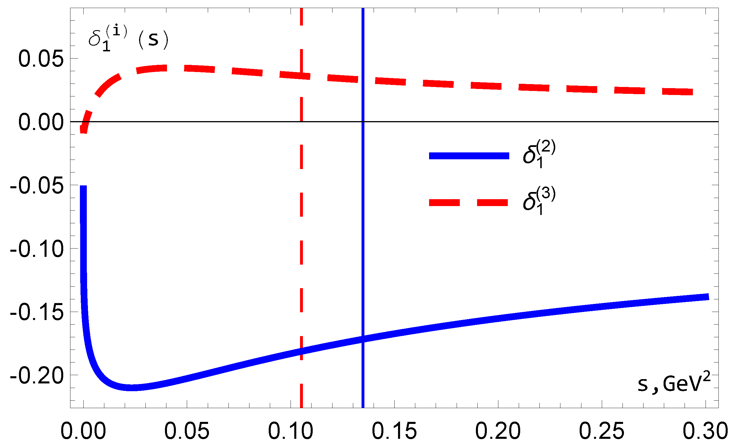
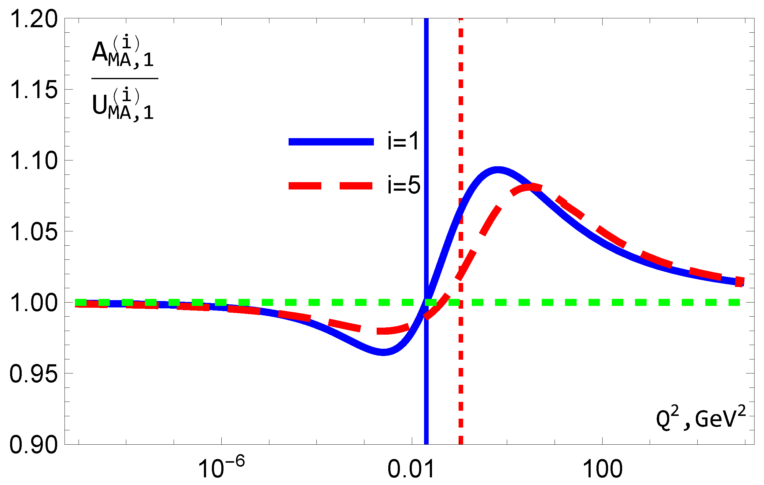
Figure 13.
The relation for . The vertical lines indicate .
Figure 13.
The relation for . The vertical lines indicate .
Figure 14.
The results for with and 4 in the framework of the usual PT and FAPT.
Figure 14.
The results for with and 4 in the framework of the usual PT and FAPT.
Figure 15.
The results for in the first four orders of PT.
Figure 15.
The results for in the first four orders of PT.
Figure 16.
The results for in the first four orders of APT.
Figure 16.
The results for in the first four orders of APT.
Figure 17.
Same as in
Figure 16 but for
0.6 GeV
2.
Figure 17.
Same as in
Figure 16 but for
0.6 GeV
2.
Figure 18.
The results for in the first four orders of APT from fits of experimental data with 0.6 GeV2
Figure 18.
The results for in the first four orders of APT from fits of experimental data with 0.6 GeV2
Figure 19.
The results for
(
122) in the first four orders of APT.
Figure 19.
The results for
(
122) in the first four orders of APT.
Figure 20.
As in
Figure 19 but for
0.6 GeV
2
Figure 20.
As in
Figure 19 but for
0.6 GeV
2
Table 1.
The values of the fit parameters in (
110).
Table 1.
The values of the fit parameters in (
110).
| |
[GeV2] for GeV2
|
for GeV2
|
for GeV2
|
| |
(for GeV2) |
(for GeV2) |
(for GeV2) |
| LO |
0.472 ± 0.035 |
-0.212 ± 0.006 |
0.667 |
| |
(1.631 ± 0.301) |
(-0.166 ± 0.001) |
(0.789) |
| NLO |
0.414 ± 0.035 |
-0.206 ± 0.008 |
0.728 |
| |
(1.545 ± 0.287) |
(-0.155 ± 0.001) |
(0.757) |
| N2LO |
0.397 ± 0.034 |
-0.208± 0.008 |
0.746 |
| |
(1.417 ± 0.241) |
(-0.156 ± 0.002) |
(0.728) |
| N3LO |
0.394 ± 0.034 |
-0.209 ± 0.008 |
0.754 |
| |
(1.429 ± 0.248) |
(-0.157 ± 0.002) |
(0.747) |
| N4LO |
0.397 ± 0.035 |
-0.208 ± 0.007 |
0.753 |
| |
(1.462 ± 0.259) |
(-0.157 ± 0.001) |
(0.754) |
Table 2.
The values of the fit parameters.
Table 2.
The values of the fit parameters.
| |
[GeV2] for GeV2
|
for GeV2
|
| |
(for GeV2) |
(for GeV2) |
| LO |
0.383 ± 0.014 (0.576 ± 0.046) |
0.572 (0.575) |
| NLO |
0.394 ± 0.013 (0.464 ± 0.039) |
0.586 (0.590) |
| N2LO |
0.328 ± 0.014 (0.459 ± 0.038) |
0.617 (0.584) |
| N3LO |
0.330 ± 0.014 (0.464 ± 0.039) |
0.629 (0.582) |
| N4LO |
0.331 ± 0.013 (0.465 ± 0.039) |
0.625 (0.584) |