
Submitted:
18 December 2024
Posted:
19 December 2024
You are already at the latest version
Abstract
We do not know how the earliest musical instruments -such as idiophones and aerophones- were played, but their acoustic properties can provide valuable clues. As a first step, we present here dissonance curves for a sound of a given spectrum. These curves show the relative dissonance that results for all intervals of a given instrument. This then leads to the association of spectra and scales, which are related because the dissonance curve has minima in the intervals that define the scale. A computational method for calculating dissonance curves is presented and several examples of its use in practical cases, both for Western and Eastern musical instruments, are given and interpreted. These results allow us to explain from a physical point of view the existence of well-known modern twelve note scales, as well as some uncommon but documented scales for various instruments in early musical history.
Keywords:
Musical acoustics
; musical instruments
; dissonance
; musical scale
; spectrum
1. Introduction
Idiophones for rhythm and aerophones for melody are probably what our ancestors played over 50,000 years ago [1]. The evolution of ancient musicality is unknown, but we can try to deduce how early musical instruments sounded by analyzing their acoustic properties and combining this with the importance of their tuning and temperament [2].
Archaeological sites have revealed many musical instruments made of stone, bone, wood or metal. All civilizations have developed such instruments simultaneously and although Western and Eastern music partly developed independently, we can find common ground in both musical areas by comparing ancient instruments developed in both geographical ends.
Documented styles and scales of early idiophones such as the Javanese gambang or the Thai renat [3] in the East and the Gambian bala or the Basque txalaparta in the West [4,5] seem to be absolutely different. Although their respective cultures have evolved separately we may find similar instruments whose acoustic principles we can analyze.
Thai culture has been in contact with other civilizations for centuries, and Thai music and musical instruments have been influenced by China, Indonesia and India, among others. Some of the musical instruments used in Thai classical music are a type of xylophone (the renat ek and its low-pitched version, the renat thum), and melodic aerophones such as the pi and other melodic instruments such as the jakeh (a type of zither).
The txalaparta is an ancient idiophone, originally from the Basque Country (european region in the Western Pyrenees) whose peculiarities as a percussion instrument and its mysterious history have aroused great interest among musicologists and historians. The first historical reference to the txalaparta appears in 1882 in a book on cider production in the Basque Country ([6], p. 129), although there are earlier mentions of toberas (a metal variant of the txalaparta). The first of these is in a legal document from 1688 ([7], pp. 52-53). Melodic instruments such as the alboka (an ancient type of clarinet) were mentioned in 1443 in the Basque Country [8]. Very little is known about the practice of the txalaparta and alboka before the 20th century, but anthropologists, historians, musicians and other scholars have placed the instrument on a new path of growth, use and cultural renewal of great international interest.
Music is usually considered to be a purely social science, belonging only to the humanities, since it deals with knowledge considered to have been invented by and for mankind. The fact that certain musical scales exist is still an important study for musicologists, anthropologists or psychologists [9]. Other social scientists also study related musical properties, such as consonance or dissonance of sound, also approaching the study of human musicality [10] and the tuning of musical instruments as an aspect mainly related to human preference [11]. The study of cultural preference or musical psychoacoustics [12] is an area that still requires much research. Important advances in the perception of familiar or unfamiliar music [13] and human preferences for musical harmony [14] have been made by researchers in multidisciplinary fields.
The existence of certain musical scales and the associated tuning of musical instruments can be treated from the point of view of acoustics as a branch of applied physics. Our approach here is based on the basic acoustic properties of both modern idiophones as well as some ancient musical instruments, which can give us some insight into how they might have been played. The study is structured as follows: Section 2 introduces Materials and Methods, including a brief review of the classical identification of dissonance applied to musical sounds. Then, Section 2.1 presents a basic method for calculating dissonance in sounds of any spectrum, and we propose a computational technique for easy calculation of dissonance curves. In Section 3 Results of the method applied to both harmonic and non-harmonic instruments are given. In particular it is shown how the well-known modern twelve semitone scale, approximately equal tempered, is obtained directly. Also, by applying the dissonance curves to modern xylophones, valuable interpretations of their musical characteristics are derived. In Section 3.3 the proposed technique is applied to the non-harmonic renat and txalaparta and their related traditional Thai and Basque instruments, respectively. Interesting features of these ancient instruments as well as appropriate but uncommon scales for their use are found. In the final section the obtained results are discussed and the main conclusions of the study are summarized.
2. Materials and Methods
One of the most famous studies of the perception of consonance and dissonance in music was by H. Helmholtz [15], who proposed a model of dissonance based on the phenomenon of beats. When two pure tones of close frequencies sound simultaneously, the interference of the two tones produces beats. The beats become slower as the frequencies of the tones become more similar, and disappear when the frequencies coincide. Slow beats are typically perceived as smooth waves, but fast beats tend to be rough and unpleasant, with maximum roughness observed when the beats occur around 32 times per second. Considering that every sound can be broken down into sinusoidal partials, Helmholtz concluded that the dissonance perceived when listening to two tones simultaneously is caused by the rapid beating of the partials. Thus, according to Helmholtz, consonance is the absence of such dissonant beats.
Assuming that the roughness of all interacting partials of two tones add up, the dissonance of any interval can be calculated simply by considering all possible combinations of pairs of partials and summing their contributions. Helmholtz performed this type of calculation for harmonic sounds such as those produced by violins [16], and presented the results graphically in diagrams such as the one shown in Figure 1, taken directly from [15]. The horizontal axis represents the interval between the two tones. One remains at a constant frequency (labelled ), and the other one moves from to the upper octave (labelled ). The height of the curves (vertical axis) is proportional to the roughness produced by the partials whose frequency ratios are labelled on the plot, using the maximum roughness criterion for 32 Hz beats. The result is a plot that has minima (intervals where minimum roughness occurs) near many of the intervals of the major scale, suggesting a relationship between the phenomenon of beats and the musical notions of consonance and dissonance.
Helmholtz’s work was of enormous importance and opened up many avenues in psychoacoustic research, many of which are still being developed. One of the most famous refinements of Helmholtz’s work on consonance and dissonance is due to R. Plomp and W.J.M. Levelt [17], who carried out a series of experiments on the perception of consonance and dissonance sensations on volunteers with no musical knowledge, using two pure tones whose relative dissonance was judged by the listeners. These experiments with pure tones made it possible to refine Helmholtz’s 32 Hz criterion and to use more closely the concept of critical bandwidth, which is not independent of the frequency. Based on their results, Plomp and Levelt were able to calculate dissonance curves for non-pure harmonic tones.
According to the theoretical procedure described in [18], which in turn builds on the work of Plomp and Levelt [17], we present a computational method for calculating general dissonance curves. The method allows the calculation of dissonance curves for both harmonic and non-harmonic sounds. This makes it possible to relate a sound spectrum (of an instrument) to a musical scale (defined by intervals that have dissonance minima).
2.1. Calculation of Dissonance Curves
Next, we show the calculation method for obtaining dissonance curves. The first step in obtaining a closed form for calculating dissonance as a function of interval is to encapsulate Plomp and Levelt’s pure tone curve in a mathematical formula. The dissonance curve for two simultaneous pure tones obtained experimentally by Plomp and Levelt (Figure 2) can be conveniently parameterized by a model of the form:
where x represents the frequency difference between the two sinusoids, and and determine how quickly the curves rise and fall. Using a least squares fit, the respective values for and are obtained.
On the other hand, the Plomp-Levelt curves depend on the absolute frequency (and not only on the difference between the frequencies of the two tones), as shown in Figure 3. This family of curves can be expressed in a single functional as described in [18]:
where y are the frequencies () of the sinusoidal tones and and are the respective amplitudes. The parameter s has the form:
where is the maximum of (1). For the above values for and this results that . The parameters s in (3) allow the functional to interpolate between the different curves in Figure 3, by moving the dissonance curve along the frequency axis so that it starts at and that the maximum dissonance occurs at the corresponding frequency. Using the Plomp-Levelt curves, the parameters can be adjusted to the values of and .
In general, a sound F of fundamental frequency is a collection of n sine waves of frecuencies and amplitudes , so that the intrinsic dissonance of F can be calculated as the sum of the dissonances of all the pairs of partials:
Finally, if two tones of F sound simultaneously in an interval of ratio (i.e. F and sound, where contains the frequencies , with amplitudes ), then the dissonance of F in the interval will be the sum of the two intrinsic dissonances of the two tones, plus the sum of the dissonances of the pairs of partials taken one at each tone:
Thus, the dissonance curve generated by F is defined as the function in all intervals of interest .
3. Results
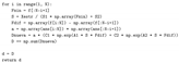
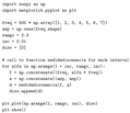
In the Appendix A we list the Python programs that have been developed and that will be used to generate the dissonance curves in this Results section. The main calculation is obtained through the code shown in Appendix A.1. This code takes a vector of frequencies and amplitudes as arguments and calculates the dissonance according to the method described above. The main program -shown in Appendix A.2- calls repeatedly the previous function for the parameters defining the corresponding sound spectrum we want to consider.
These compact codes allow very fast and efficient calculation of dissonance curves for arbitrary sounds, and will be used in the following to obtain the results. The dissonance curves can be calculated to describe the expected characteristics of general kind of musical instruments taking into account their corresponding spectra.
3.1. Dissonance Curves for Harmonic Sounds
Using the proposed computational model listed in the Appendix A, Figure 4 is calculated, which is the dissonance curve corresponding to a harmonic sound with a fundamental frequency of 500 Hz and six additional harmonics. The result is very illustrative. As it can be seen, the curve has minima where the frequencies are related by simple ratios. In addition, the consonant intervals of the octave (), the perfect fifth (), the major sixth (), the perfect fourth (), and the major and minor thirds ( and , respectively) stand out. Other intervals that can be approximately identified are the augmented sixth (about ), the augmented fourth (about ) and the major second (about ). Finally, the dissonant intervals of the minor second (approximately ), minor sixth () and seventh (approximately ) are also identified.
Overall, the dissonance curve for harmonic sounds allows the definition of the twelve semitone scale in common use, simply by identifying the intervals of the scale of minimum dissonance. In this sense, it can be said that the harmonic spectrum and the twelve semitone scale (typical of most modern Western musical instruments) are closely related.
3.2. Dissonance Curve for Xylophone Bars
Having applied the method of dissonance curves to harmonic sounds, we can now ask what consonances and dissonances are to be expected when non-harmonic spectrum instruments are used. In this sense, it is quite possible that intervals that are commonly considered to be consonant or dissonant will change their characteristics when played on non-harmonic instruments. It is also possible that, given the dissonance curve of a non-harmonic instrument being studied, a more appropriate associated scale can be defined, better than the usual one of twelve approximately equal tempered tones.
The following application result studies the experimental response spectrum of xylophone bars presented in [19]. According to these experimental data, the response of a ’Royal Percussion’ Studio-49 (Germany) xylophone bar tuned to an A4 is not harmonic and has a spectrum:
Using these data, and assuming that all partials have the same amplitude for simplicity, the dissonance curve shown in Figure 5 is calculated. The dissonance predicted by the curve is generally lower than that of the harmonic tones (compare Figure 5 and Figure 4). Perhaps the most notable differences between the two curves are the relative dissonance expected for the major sixth interval (interval 1.67) and the predicted consonance for the seventh interval (interval 1.89) in the xylophone bars, both of which are the opposite for the harmonic sounds.
Using the data from [19] again to weight the relative contribution of the partials, their relative amplitudes in the spectrum of the measured bars are approximately as follows:
3.3. Application to East and West Traditional Instruments
The ordinary Basque txalaparta consists of wooden planks laid horizontally on two supports and struck with wooden sticks by four hands. Due to the rural origins of the instrument, it is very common to use planks from local trees such as oak, chestnut or alder, and ash sticks, similar to the short handles of rural tools. The metal bar used in the old smithies of the Basque Country was a bronze tube weighing several kilos, with a slightly flattened conical shape, and as such it had all the prerequisites for good sonority of the toberas. According to all the evidence, this must have been the instrument that was originally played at weddings. This percussion instrument has been used together with aerophones such as the alboka capable of providing penta or heptatonic melodies.
A surprising aspect of traditional Thai music is that it is played in a scale that is very close to an equal tempered heptatonic scale, which means that its intervals never coincide (except in the octave) with those of the twelve semitone equal tempered scale. The renat, for example, is a xylophone tuned approximately to a single equal tempered heptatonic scale. The modes of vibration of the renat bars and the txalaparta planks are similar to those of an ideal bar, whose spectrum contains the following first four partials [20]:
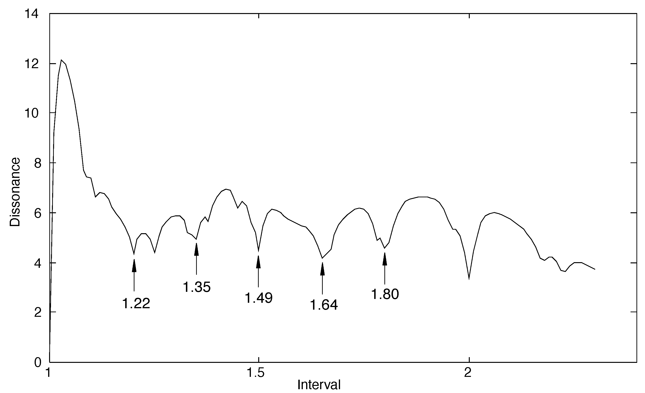
Combining this with a harmonic sound such as the pi, the jakeh or the alboka and taking six partials, it can be calculated the mixed dissonance curve that would be produced by playing melodic and percussion instruments together (Figure 7). As it can be seen in the plot, the curve has dissonance minima in the following intervals:
which largely coincides with the division of the octave into the rather uncommon seven equal tempered scale based on intervals :
so that the proposed acoustical model based on dissonance curves provides an explanation of the documented use of the unusual seven equal tempered musical scale in ancient music.
4. Discussion
Several remarkable findings have been presented in the previous Results section using the dissonance curves of harmonic or non-harmonic musical instruments. Instead of using the classical Pythagorean or modern twelve equal tempered musical scales [2], we have based our study on the basic acoustic properties and spectra of musical instruments to construct dissonance curves. The dissonance minima have allowed us to explain musical scales not as a pure human invention [1], but as an approach based on musical acoustics of musical instruments and the biological rationale for musical scales [9] and musical consonance [10]. The heptatonic scale and the spectrum of traditional Thai [3] and Basque instruments [5] are associated in the sense used in this study, which provides arguments to try to explain the use of this scale in the aforementioned traditional music.
By studying the dissonance curves of modern xylophones, we can see that they have evolved into symphonic idiophones, which can be used in conjunction with all kinds of instruments and scales, either with the modern twelve semitone equal tempered scale of Western music, or with the introduction of Eastern microtones. However, the ancient rhythmic idiophones, both Western and Eastern, by their very acoustic nature, allow us to explain how the rather uncommon but well documented [3] equal tempered heptatonic scale arises, which fits perfectly with their contemporary melodic aerophones, such as the Thai pi or the Basque alboka, respectively.
This study has introduced the idea of the dissonance curve of a given spectrum sound and has presented a computationally efficient method for calculating such curves. It has been shown how the twelve-tone (approximately equal tempered) musical scale is related to the (harmonic) spectrum of most musical instruments in the sense that its dissonance curve has minima in the intervals of the scale.
In addition, the method of dissonance curves has been used in several examples of instruments involving both harmonic and non-harmonic spectra. It has been shown how modern xylophones have evolved to reach true symphonic characteristics, that can coexist with any oriental or western musical instruments.
Finally, an application of the dissonance curve method to traditional Thai and Basque instruments has provided a simple explanation for the initially surprising fact that the equal heptatonic scale is widely used in Thai music, and that a traditional aerophone such as the alboka, capable of producing just simple pentatonic or heptatonic melodies, fits perfectly well with ancient percussion Basque idiophones such as the txalaparta.
Funding
This research was funded by the Basque Goverment grant number IT1533-22.
Conflicts of Interest
The authors declare no conflicts of interest.
Appendix A.
Appendix A.1. Program Code for Computation of Dissonance Curves
First, we present a function called medidadisonancia, which takes as arguments a vector of frequencies and amplitudes and calculates the dissonance according to the method described above:

Appendix A.2. Calling Code to Compute and Plot Dissonance Curves
The above function is called repeatedly from a main program in which the sound spectrum is defined. For example, the following program draws the dissonance curve for a harmonic sound with a fundamental frequency of 500 Hz and six harmonics, all of equal amplitude:
References
- Morley, I. The Prehistory of Music: Human Evolution, Archaeology, and the Origins of Musicality; Oxford University Press, 2013. [Google Scholar]
- Murray Barbour, J. Tuning and Temperament: A Historical Survey; Dover Publications Inc.: New York, 1951. [Google Scholar]
- Morton, D. The traditional music of Thailand; University of California Press: Berkeley, 1976. [Google Scholar]
- Jones, A. Africa and Indonesia: the evidence of xylophone and other musical and cultural factors; E.J. Brill: Leiden, 1971. [Google Scholar]
- Beltran, J.M. Txalaparta (in spanish and basque); Nerea: San Sebastian, Spain, 2013. [Google Scholar]
- Aguirre-Miramon, S. Cider production in the provinces of the Basque Country (in spanish); Hijos de I.R. Baroja: San Sebastian, Spain, 1882; p. 129. [Google Scholar]
- Lekuona, M. The toberas (in spanish). Revista de cultura vasca, Euskalerriaren Alde 1920, 194, 52–53. [Google Scholar]
- Donostia, J.A. Musical instruments of the Basque people (in spanish); Icharopena: Zarauz, Spain, 1952. [Google Scholar]
- Gill, K. Z.; Purves, D. A biological rationale for musical scales. PLoS ONE 2009, 4, e8144. [Google Scholar] [CrossRef] [PubMed]
- Bowling, D. L.; Purves, D. A biological rationale for musical consonance. Proc. Natl Acad. Sci 2015, 112, 11155–11160. [Google Scholar] [CrossRef] [PubMed]
- Friedman, R. S.; Kowalewski, D. A.; Vuvan, D. T.; Neill, W. T. Consonance preferences within an unconventional tuning system. Music Percept 2021, 38, 313–330. [Google Scholar] [CrossRef]
- Eerola, T.; Lahdelma, I. The anatomy of consonance/dissonance: evaluating acoustic and cultural predictors across multiple datasets with chords. Music Sci 2021, 4. [Google Scholar] [CrossRef]
- Smit, E. A.; Milne, A. J. The need for composite models of music perception: consonance in tuning systems (familiar or unfamiliar) cannot be explained by a single predictor. Music Percept 2021, 38, 335–336. [Google Scholar] [CrossRef]
- Stolzenburg, F. Harmony perception by periodicity detection. J. Math. Music 2015, 9, 215–238. [Google Scholar] [CrossRef]
- Helmholtz, H. On the sensations of tone; Dover Publications Inc.: New York, 1954. [Google Scholar]
- Etxebarria, V.; Riera, I. Measuring the frequency response of musical instruments with a PC-based system. Catgut Acoustical Society Journal 2002, 4, 26–30. [Google Scholar]
- Plomp, R.; Levelt, W.J.M. Tonal consonance and critical bandwidth. Journal of the Acoustical Society of America 1965, 38, 548–560. [Google Scholar] [CrossRef] [PubMed]
- Sethares, W.A. Local consonance and the relationship between timbre and scale. Journal of the Acoustical Society of America 1993, 94, 1218–1228. [Google Scholar] [CrossRef]
- Bretos, J.; Santamaria., C.; Alonso Moral, J. Frequencies, input admittances and bandwidths of the natural bending eigenmodes in xylophone bars. Journal of Sound and Vibration 1997, 203, 1–9. [Google Scholar] [CrossRef]
- Fletcher, N.H.; Rossing, T.D. The Physics of Musical Instruments, 2nd Edition ed; Springer: New York, 1998; pp. 628–629. [Google Scholar]
Figure 1.
Areas of roughness calculated and plotted by H. Helmholtz (1870) when two violin notes are played simultaneously, to explain the consonance and the dissonance of sounds produced by musical instruments with harmonic spectra. (Reproduced from the english translation [15] p. 193).
Figure 1.
Areas of roughness calculated and plotted by H. Helmholtz (1870) when two violin notes are played simultaneously, to explain the consonance and the dissonance of sounds produced by musical instruments with harmonic spectra. (Reproduced from the english translation [15] p. 193).
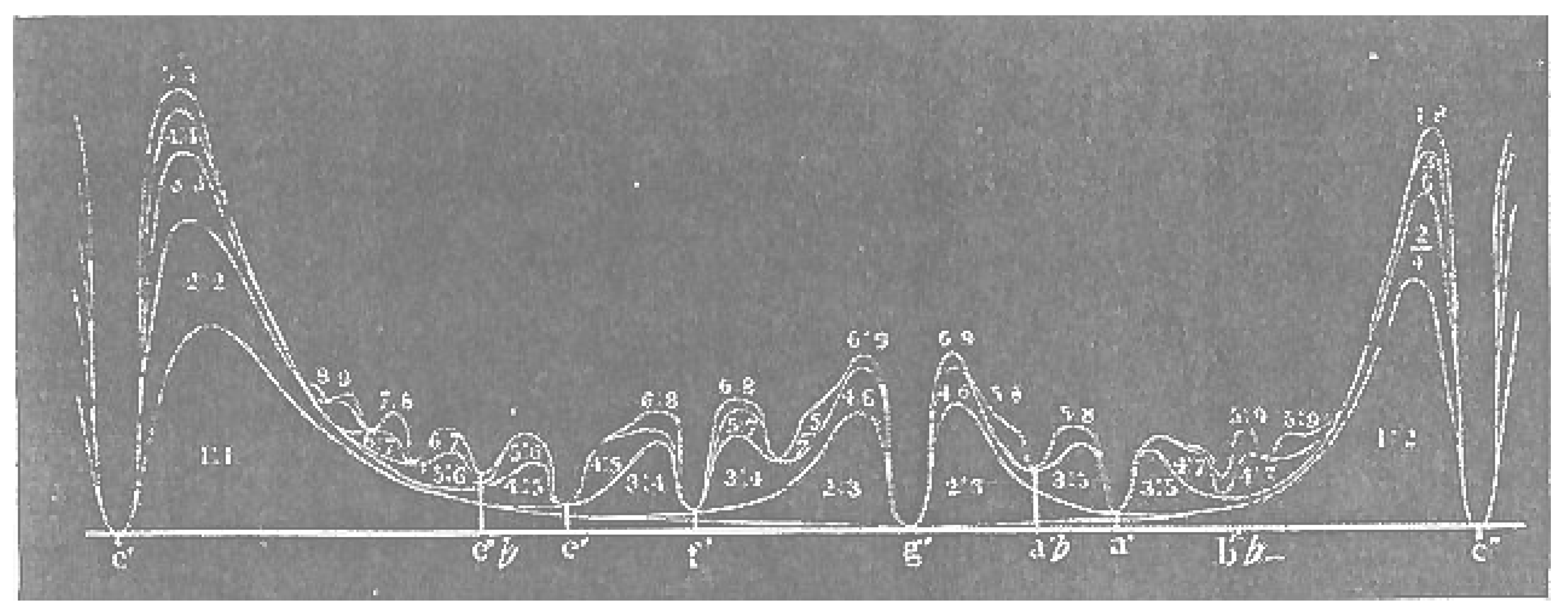
Figure 2.
Parametrization model for the dissonances observed by Plomp and Levelt [17] in a series of experiments of two simultaneous pure tones sounding at close frequencies, to refine the phenomenon of beats observed by Helmholtz and its corresponding effect in perception of dissonance and consonance.
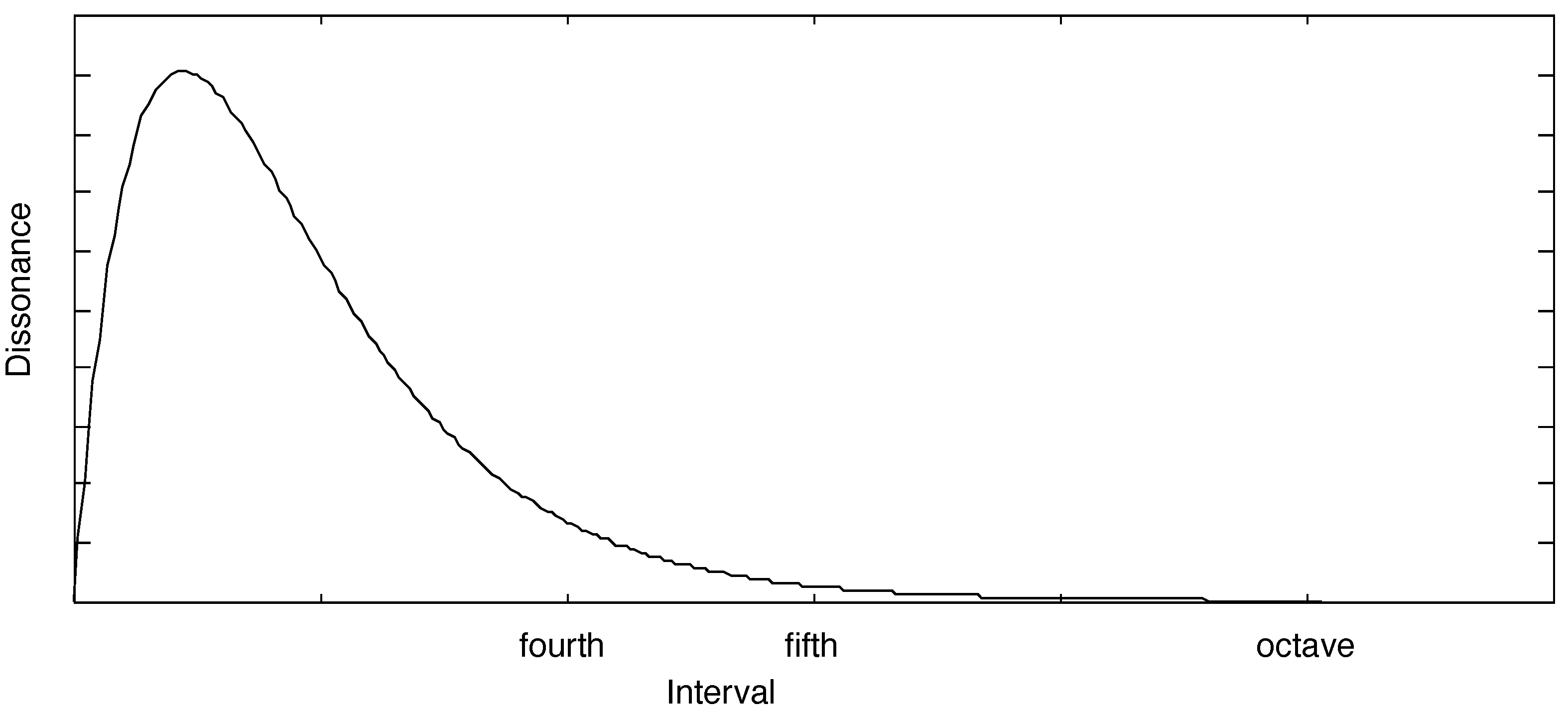
Figure 3.
Plomp-Levelt dissonance curves in experiments for different base frequencies [17]. It is observed that the dissonance depends not only on the difference between the frequencies of the two pure tones, but on the absolute frequency as well.
Figure 3.
Plomp-Levelt dissonance curves in experiments for different base frequencies [17]. It is observed that the dissonance depends not only on the difference between the frequencies of the two pure tones, but on the absolute frequency as well.
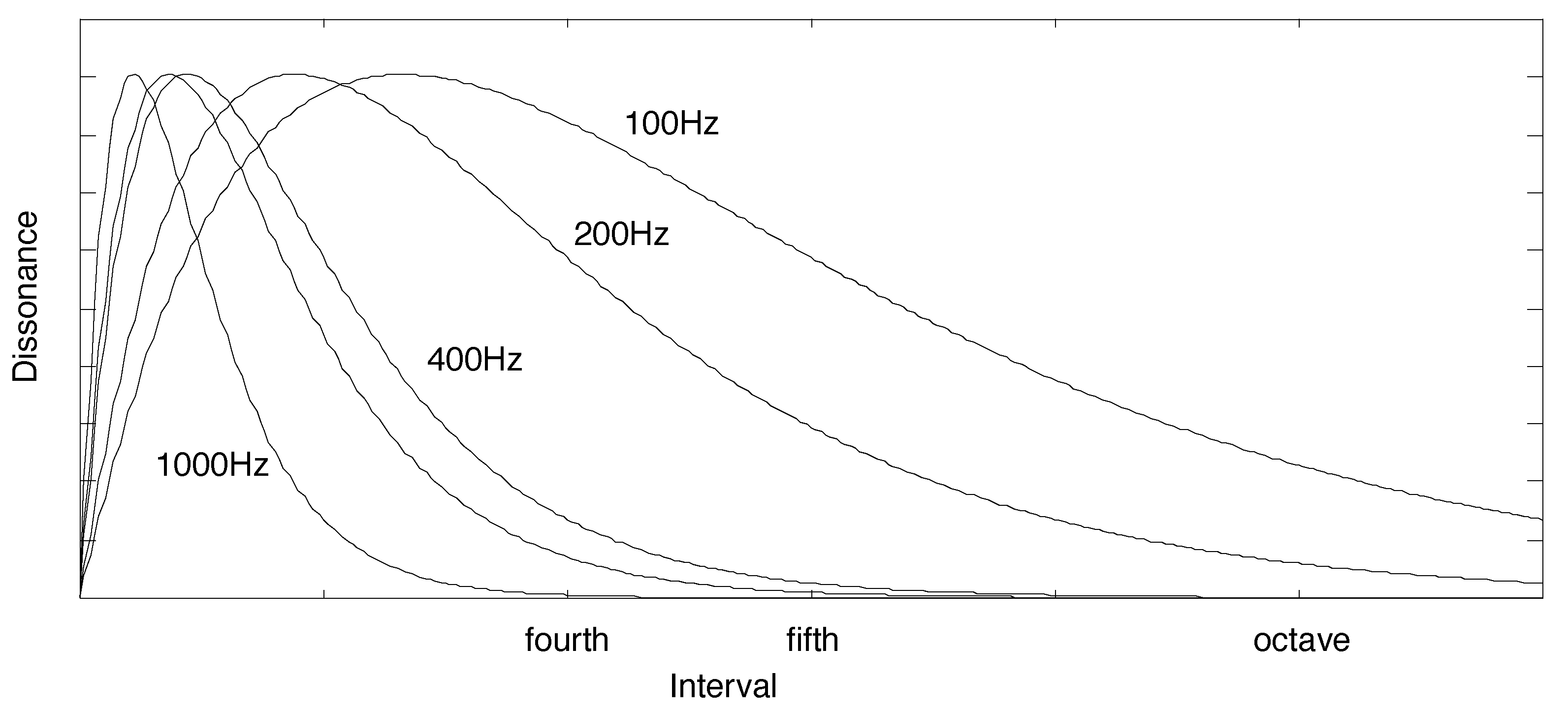
Figure 4.
Dissonance curve calculated using the proposed computational model for a harmonic sound with a fundamental frequency and six additional harmonics. From this result it is very important the finding that the dissonance minima coincide very closely with the well-known twelve musical intervals. This reveals the clear association between musical scales and dissonance.
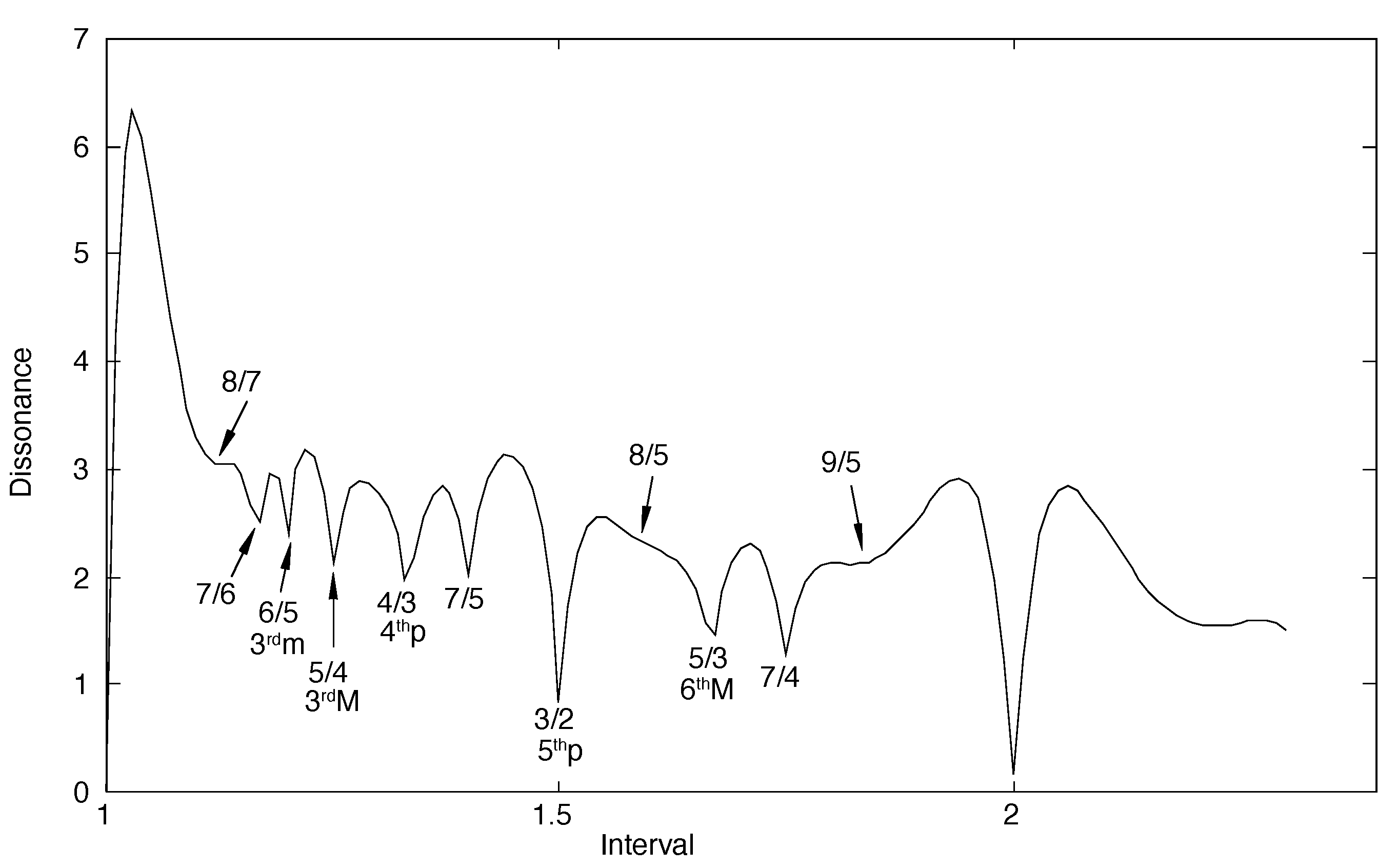
Figure 5.
Dissonance curve calculated using the proposed computational model for the non-harmonic spectrum sound of the modern ’Royal Percussion’ Studio-49 (Germany) xylophone. From this result, as expected, the harmonic and non-harmonic instruments result in quite different dissonance curves.
Figure 5.
Dissonance curve calculated using the proposed computational model for the non-harmonic spectrum sound of the modern ’Royal Percussion’ Studio-49 (Germany) xylophone. From this result, as expected, the harmonic and non-harmonic instruments result in quite different dissonance curves.
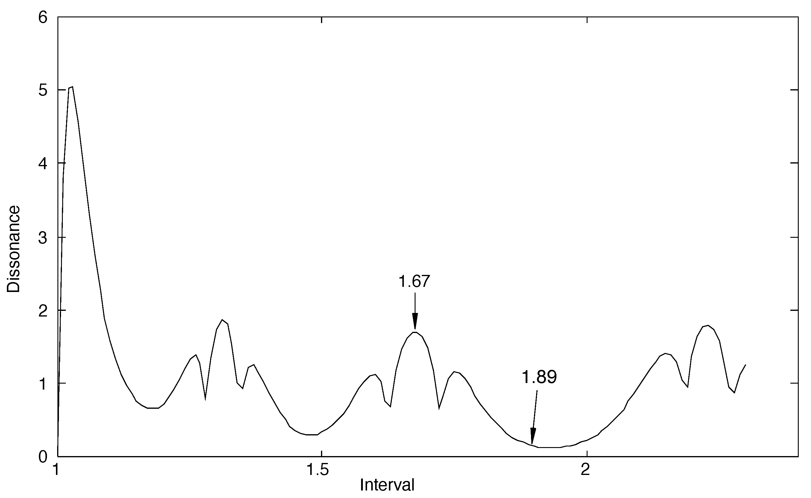
Figure 6.
Dissonance curve calculated using the proposed computational model for the non-harmonic spectrum sound of the modern ’Royal Percussion’ Studio-49 (Germany) xylophone, using the measured real decreasing amplitudes. From this result, it is found that the dissonance decreases for all intervals, and thus the modern xylophone, even though starting from a non-harmonic spectrum, may fit with any other kind of symphonic instruments.
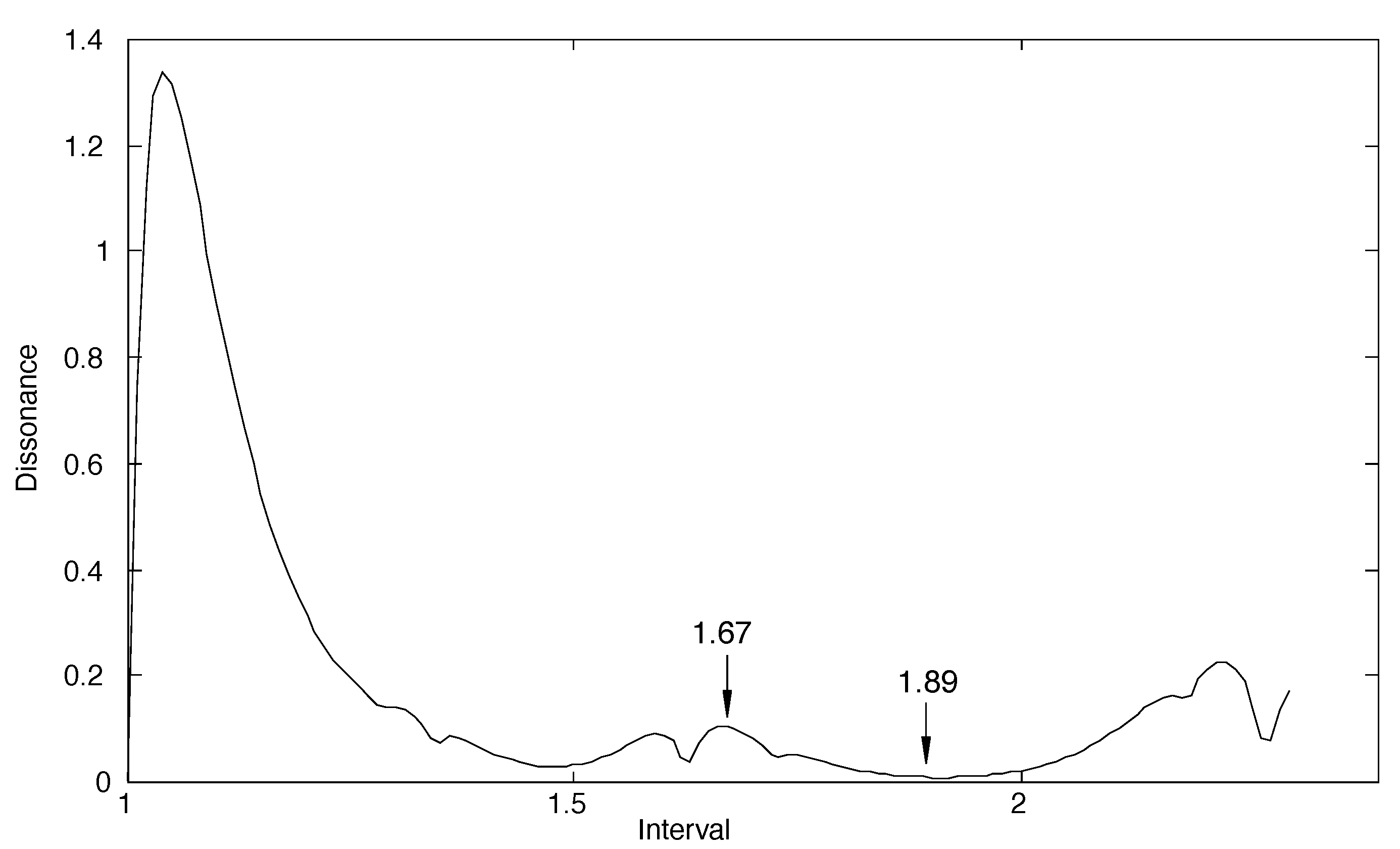
Figure 7.
Dissonance curve calculated using the proposed computational model for the non-harmonic spectrum sound of the Basque txalaparta and alboka or the Thai renat and jakeh. From this result, it is found the remarkable fact that these rustic ancient instruments fit perfectly well with the rather uncommon seven equal tempered musical scale.
Disclaimer/Publisher’s Note: The statements, opinions and data contained in all publications are solely those of the individual author(s) and contributor(s) and not of MDPI and/or the editor(s). MDPI and/or the editor(s) disclaim responsibility for any injury to people or property resulting from any ideas, methods, instructions or products referred to in the content. |
© 2024 by the authors. Licensee MDPI, Basel, Switzerland. This article is an open access article distributed under the terms and conditions of the Creative Commons Attribution (CC BY) license (http://creativecommons.org/licenses/by/4.0/).
Copyright: This open access article is published under a Creative Commons CC BY 4.0 license, which permit the free download, distribution, and reuse, provided that the author and preprint are cited in any reuse.


