
Submitted:
12 December 2024
Posted:
12 December 2024
You are already at the latest version
Abstract
This study examines an atmospheric bore formed from the collision between a colder gust front (GF) and a warmer sea breeze (SB) over the Bohai sea coast of China during the night of June 12-13, 2018. Utilizing radar data, ground-based observations, and high-resolution numerical simulations, the findings indicate that the approaching SB establishes a stabilizing boundary layer (SBL) into which the GF from the convective downdraft intrudes, transitioning from a density current to a non-undular bore and eventually to an undular one. The undular bore then propagates within favorable trapping layers associated with the SB, facilitating convection initiation (CI). Dynamics governing this bore formation process are also investigated and validated using laboratory model theories. Results also reveal that the structure of the mesoscale convective system (MCS) is significantly influenced by the presence of the bore. Substantial convective available potential energy (CAPE) -rich air parcels within the SBL are lifted by the bore, fueling the MCS and lead to CI, thereby sustaining the MCS's intensity and longevity. Given the prevalence of GFs and SBs over the eastern coastal regions of China, their collisions will create a high likelihood of bore formation, regardless of the environmental boundary layer conditions. This significantly enhances the potential for bores to play a crucial role in CI, particularly during the daytime.
Keywords:
atmospheric bore
; density currents collision
; mesoscale convective systems
; convection initiation
; radar data applications
; numerical simulations
1. Introduction
An atmospheric bore is a gravity wave response, often accompanied by a rise in surface pressure, a sudden shift in wind direction, and an increase in wind speed, while the temperature remains stable or experiences a slight rise [1,2,3]. The formation of atmospheric bores is closely linked to density currents, which are hydrodynamic flows driven by density differences within a fluid and serve as a crucial mechanism for mass transport [4]. Common examples of density currents include cold pool outflows, often referred to as gust fronts (GFs), and sea breezes (SBs). At night, the lower atmosphere frequently develops a stable boundary layer (SBL) due to radiative cooling. When cold pools outflows undercut the strong SBL, wave disturbances are triggered at the upper boundary of the SBL, leading to the formation of bores [5,6,7]. Additionally, the collision of density currents can generate bores. Notable examples include the collision of two sea breeze fronts (SBFs) [8,9,10,11,12], the collision of a gust front (GF) with a SBF [13,14], the meeting of two GFs [15], and the convergence of a GF with a cold front [16]. Based on laboratory experiments, Simpson (1997) pioneered a conceptual model for bore formation resulting from density current collisions [4]. He found that under ideal conditions, when two density currents of equal density collide, a symmetrical "hump" emerges at the point of impact. However, in real-world scenarios, it is more common for density currents of different densities to collide. In such cases, the denser fluid tends to undercut the less dense one, causing it to bulge and lift, which in turn forms two opposing bores.
Numerous studies [17,18,19,20,21,22,23,24] have shown that bores favor convection initiation (CI) by lifting unstable air parcels or by reducing convective inhibition (CIN) and the level of free convection (LFC). This phenomenon was a key focus of the Plains Elevated Convection at Night (PECAN) field study in 2015, which aimed to explore the impact of frequent bores on CI and their role in sustaining mesoscale convective systems (MCSs) over the Southern Great Plains (SGP) of the United States [25]. During PECAN, bores were associated with approximately 25% of the elevated CI events [26]. It is evident that a longer lifespan of a bore is correlated with a more sustained MCS. The key to sustaining bores as gravity disturbances lie in preventing the vertical propagation of fluctuating energy, thus enabling the fluctuations to propagate horizontally. Scorer (1949) noted that energy trapping within fluctuations can occur through reflections (i.e., waveguide), and introduced the Scorer parameter () to analyze the maintenance of gravity waves [27]. Vertical fluctuations can be trapped when transitions from positive to negative with height [6]. Recent studies [23,24,28] have further indicated that long-lived bores are often associated with a strong nocturnal low-level jet (LLJ), as wave energy is effectively captured when LLJs move in the opposite direction to the bores.
Bores have been documented in various regions worldwide, including China [3,29,30,31,32,33]. Zhang, Parsons, and Xu et al. (2020) conducted the first dynamic study on the formation and evolution of atmospheric bores observed over the Yangtze-Huaihe Plain, demonstrating that atmospheric bores can form nocturnally in China and the characteristics of them are more distinctive compared to those in other regions, such as SGP [23]. Bores are classified by strength into three types: Type A, exhibiting smooth, undular waveforms; Type B, resembling an undular bore but partially merging with features of a density current; and Type C, lacking waveforms and fully resembling a density current [34]. Zhang, Parsons, and Xu et al. (2020) observed a bore initially formed as Type C, characterized by a density current appearance, but later evolved into a strong Type B one with a wavelike structure [23]. This progression from Type C to Type B contrasts with previous studies where bores typically formed directly as Type A or Type B [7]. Building on this research, Zhang, Parsons, and Xu et al. (2022) conducted the first multi-year statistical study on bores over the Southern North China Plain (SNCP) during the warm seasons from 2015 to 2019 China [33]. They found that while the SNCP experiences fewer bores than the SGP, the occurrences are more spatially widespread. The lower bore frequency over the SNCP highlights the environmental diversity of this region, and it is hypothesized that bore formations in China may be more complex, potentially due to the higher moisture levels across the plains, which are less conducive for the formation of strong cold pool. In their recent study, Zhang, Parsons, and Xu et al. (2024) identified that bores over the SNCP are likely driven by interactions between strong mesoscale convective downdrafts and a strong SBL [24]. This suggests a potentially unique dynamical mechanism for bore formation in China. The research conducted in these studies [23,24,33] has laid a foundation for understanding bores across the China.
Moreover, they found that the East China Plain, with its extensive coastline, presents additional opportunities to explore bore dynamics, where convective cold pools may frequently collide with SBFs, enhancing the region's potential for diverse bores formation [24]. Density current collisions can occur at any time, allowing for bore formation even when the boundary layer is active. When stronger bores develop during collisions, they can propagate over hundreds of kilometers with minimal kinetic energy loss under ideal conditions, such as the establishing SBL from the SB, and potentially initiating additional thunderstorms [14,35]. The frequent occurrence of MCSs during warm season along China's eastern coast, along with the near-daily presence of SBFs, suggests that bores could significantly influence CI under specific conditions, such as an active boundary layer. This will represent a novel mechanism for triggering intense convection off the coast of China. Understanding how density current collisions lead to bore formation and their impact on CI in unstable boundary layer conditions is crucial. Such insights are vital for enhancing the accuracy of severe weather forecasting and issuing timely warnings.
This study represents the first exploration into the mechanism of bore formation via density current collisions along the Chinese coast. By examining an MCS’s convective outflow along the Bohai Sea coast, we documented an undular bore generated from the collisions between this outflow and a coastal SBF. This phenomenon, observed at night during the warm season, was initiated by the persistent collision between a GF and a SBF. Throughout the bore's propagation, we identified the initiations of several intense convective cells upstream, some of which merged with the MCS to maintain it, while others consistently followed the bore as it advanced eastward. Unlike previous studies, our findings revealed a well-mixed boundary layer preceding bore formation, despite the nocturnal timing of the collision. Our research aims to build upon the work of Zhang, Parsons, and Xu et al. by introducing a potential new avenue for investigating bore phenomena in the Chinese region. The remainder of this article is organized as follows: Section 2 provides an observational analysis of the bore's formation and evolution. Section 3 details a numerical simulation using the Advanced Research Weather Research and Forecasting model (ARW-WRF v4.2) [36], with comparisons between simulation results and observational data validating the model's applicability. Section 4 explores the dynamic and thermodynamic processes underlying the collision that gives rise to the bore, as well as the role of the bore in CI. Section 5 analyses the dynamics of bore formation. Section 6 summarizes the findings of the study. All times mentioned in this paper are in Local Standard Time (LST, LST = UTC + 8 hours).
2. Observation Analysis
2.1. Data
The observational data used in this study consist of two components:
(1) Radar reflectivity data obtained from two S-band radars located at Cangzhou (CZ) and Qingdao (QD). These radars have a maximum scanning range of 460 km and operate with a scanning interval of 6 minutes. The radar systems are similar in hardware and software to the Weather Surveillance Radar-1988 Doppler radars (WSR-88Ds) deployed in the United States [37].
(2) Ground-based observation data obtained from the operational ground-based monitoring network, which has a spatial resolution of approximately 25 km and a temporal resolution of 6 minutes. The dataset includes measurements of temperature, barometric pressure, wind direction, and wind speed. The precision of the temperature and pressure measurements is 0.1°C and 0.1 hPa, respectively.
2.2. Structure of the MCS and Identification of Bore
The formation, structure, and evolution of the MCS were comprehensively observed by the CZ radar (Figure 1a-c) and QD radar (Figure 1d-f) during the night of 12 June and the early hours of 13 June 2018.
Around 2200 LST, the MCS located over the western Bohai Sea, featuring a high reflectivity core exceeding 45 dBZ, oriented along a southwest-northeast axis, accompanied by extensive weaker convection under 35 dBZ trailing the system. At this time, a distinct radar reflectivity line (RFL) was observed at the leading edge of the outflow (Figure 1a), alongside a narrow SBF paralleling the Bohai Sea coastline. Notably, a mountain range with an elevation of approximately 1 km lies to the southeast of the MCS (depicted with light orange shading in Figure 1). From 2200 LST to 2300 LST (Figure 1a and b), the MCS exhibited progressive north-south development and the RFL approached the SBF, ultimately leading to their collision at their northern part. This collision resulted in rapid intensification of the system, which extended north-south from 150 km to 250 km (Figure 1b, c).
On the following day, around 0031 LST (Figure 1d), the QD radar captured final stage of the collision. By 0128 LST (Figure 1e), multiple RFLs formed taking the appearance of undular bores with several convective cells initiated upstream. Subsequently (Figure 1f), some of these convective cells merged with the parent MCS, allowing the system to maintain, while others propagated eastward following the RFLs. During this period, the system transitioned from a linear north-south MCS to a bow-shaped echo and finally merged with downstream linear convection to form a T-shaped convective system.
RFLs are well-established indicators of mesoscale boundary convergence lines, such as SBFs, GFs, and bores [38]. The transformation of a single RFL into multiple RFLs often signifies the formation of undular bore [33]. Given these observational facts, eight stations from the ground-based observation network were selected along the RFLs' trajectory (Figure 2) to qualitatively verify the bore generation resulting from the gravity currents collision.
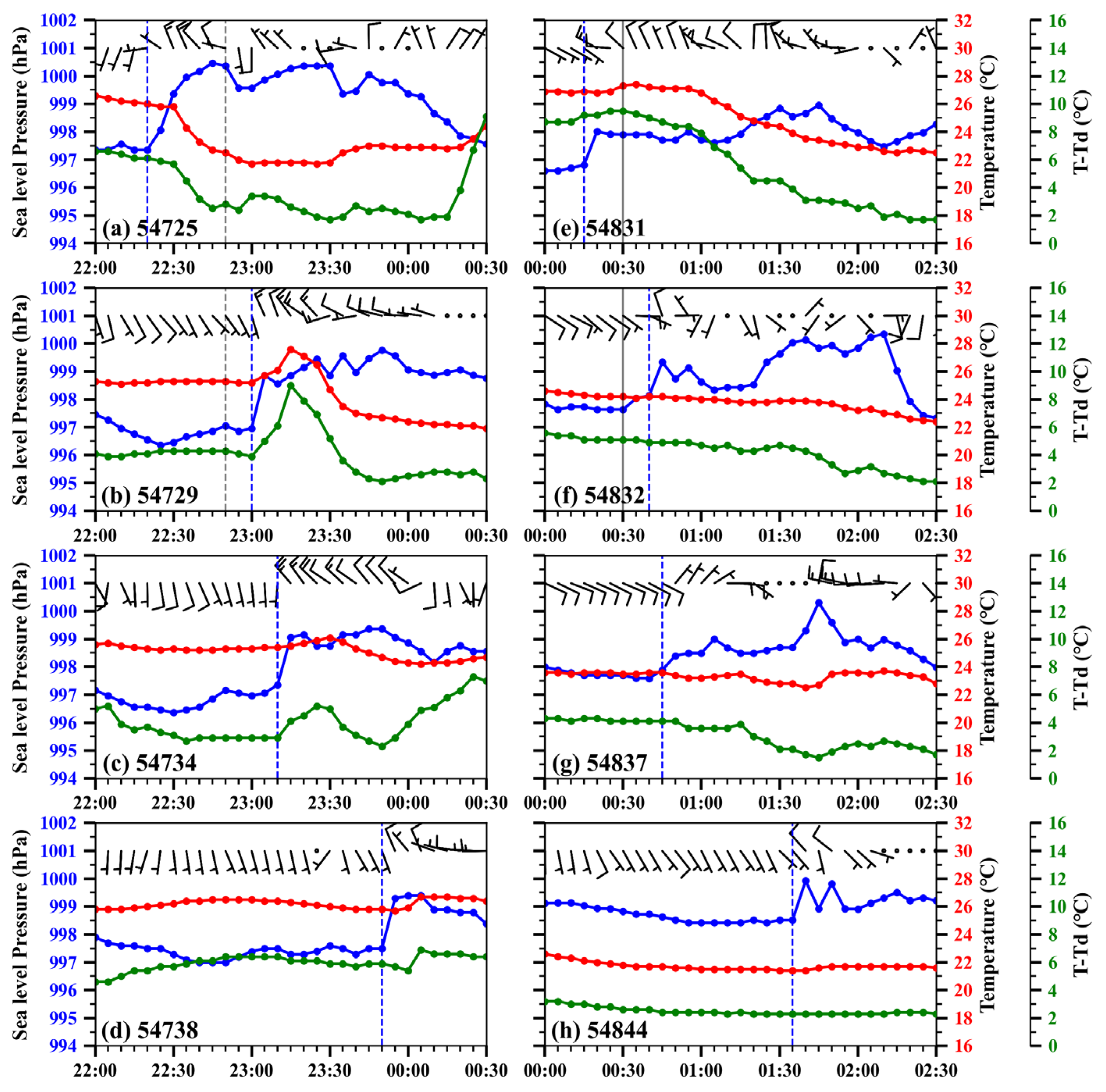
At 2220 LST, as the RFL was about to pass station 54725 (Figure 2a), a surface pressure surge of approximately 3.5 hPa, a sharp temperature drop of about 3°C, an abrupt shift in wind direction, and a significant increase in wind speed were observed. Additionally, a reduction in temperature-dewpoint difference indicated an increase in relative humidity, suggesting that the RFL observed in Figure 1a corresponded to a GF. By 2300 LST, stations 54729 (Figure 2b) and 54734 (Figure 2c) recorded a change in the character of the RFL, which now exhibited a more modest pressure increase of around 2 hPa, and a temperature that either rose slightly or remained steady. This indicated the transition of the RFL of GF into a non-undular bore, which was also later observed by stations 54738 (Figure 2d) and 54831 (Figure 2e). As the collision between the GF and the SBF neared its final stage by 0030 LST, station 54832 (Figure 2f) recorded two distinct air pressure jumps within ten minutes of the RFL's passage at 0040 LST. This suggested multiple fluctuations, coinciding with the evolution of a single RFL into multiple RFLs—a transformation from a non-undular bore to a undular bore. This evolution was also observed at nearby station 54837 (Figure 2g) and downstream at station 54844 (Figure 2h).
Throughout this process, the RFL initially acted as a GF and gradually transformed into a non-undular bore, eventually developing into an undular bore during its ongoing collision with the SBF. The collision likely began around 2240 LST (as indicated by translucent black dashed lines in Figure 2a and Figure 2b) and ended near 0030 LST (as shown by translucent black solid lines in Figure 2e and Figure 2f). This period documented a slight increase in humidity, likely due to the mixing of water vapor resulting from the GF and SBF interaction. Furthermore, the continuous collision of the GF with the SBF, along with the passage of the southern edge of the MCS over a mountain range, suggests that downslope winds associated with the mountains may have also contributed to the bore's formation by enhancing the GF and facilitating its eventual transition into an undular bore.
Figure 2.
The temperature (read line, units: °C), pressure (blue line, units: hPa), temperature-dewpoint difference (green line, units: °C) series, and observed surface wind field at selected stations (wind barbs, units: knots, half and full barbs for 2 m s⁻¹ and 4 m s⁻¹, respectively). The blue dashed lines indicate the passage of the observed RFL(s) at different directions, and the locations of the ground-based stations are shown in Figure 1a, d. The translucent black dashed lines in panels (a) and (b) indicate the temporal point at which the GF collided with the SBF, whereas the translucent black solid lines in panels (e) and (f) indicate the temporal point at which the collision concluded.
2.3. Large Scale Environment
An analysis of the large-scale synoptic conditions preceding the collision was conducted using ERA5 data, which has a temporal resolution of 1 hour and a spatial resolution of 0.25° × 0.25° [39].
At 500 hPa (Figure 3a), a low-pressure center is positioned to the northwest of the MCS, channeling west-northwesterly dry and cold air to the system. Meanwhile, total column water vapor analysis reveals favorable ambient moisture conditions to the east of the MCS. Notably, the presence of water vapor maxima to the north of MCS suggest potential development in that region, which is consistent with observation (Figure 1d-f). At the 850 hPa level (Figure 3b), the MCS located at the northern terminus of the southwest LLJ. The 2 m temperature indicates warmer conditions on the MCS's southwest side, which, coupled with the LLJ, facilitates optimal water vapor transport in the vicinity of the MCS. Consequently, the MCS was situated in an unstable, stratified atmosphere, characterized by a warm, humid low-level environment juxtaposed with a dry, cold mid-level. Additionally, significant vertical wind shear between 850 hPa and 500 hPa creates a favorable environment for sustaining the MCS and promoting CI.
Figure 3.
Geopotential height (black contours, units: dagpm) and horizontal wind fields (half and full barbs for 2 m s⁻¹ and 4 m s⁻¹, respectively) at (a) 500 hPa with total column water vapor (shaded, units: kg m-2) and (b) 850 hPa with 2 m temperature (shaded, units: °C) at 2200 LST on 12 June 2018 derived from ERA5 data. The black rectangle indicates the MCS development area, and 'L' indicates a low-pressure center. The brown color curve in panel (a) indicates the trough and the red '×' as Figure 1a. Skew-T diagram (c-f) at the red '×' in panel (a), showing profiles of ambient temperature (red line), air parcel temperature (black line), and dewpoint temperature (green line). The convective inhibition (CIN) area is shaded light blue and the convective available potential energy (CAPE) area is shaded light red. Panels (c), (d), (e), and (f) correspond to the red '×' from west to east, respectively. The ERA5 reanalysis is hourly with a spatial resolution of 0.25° × 0.25°.
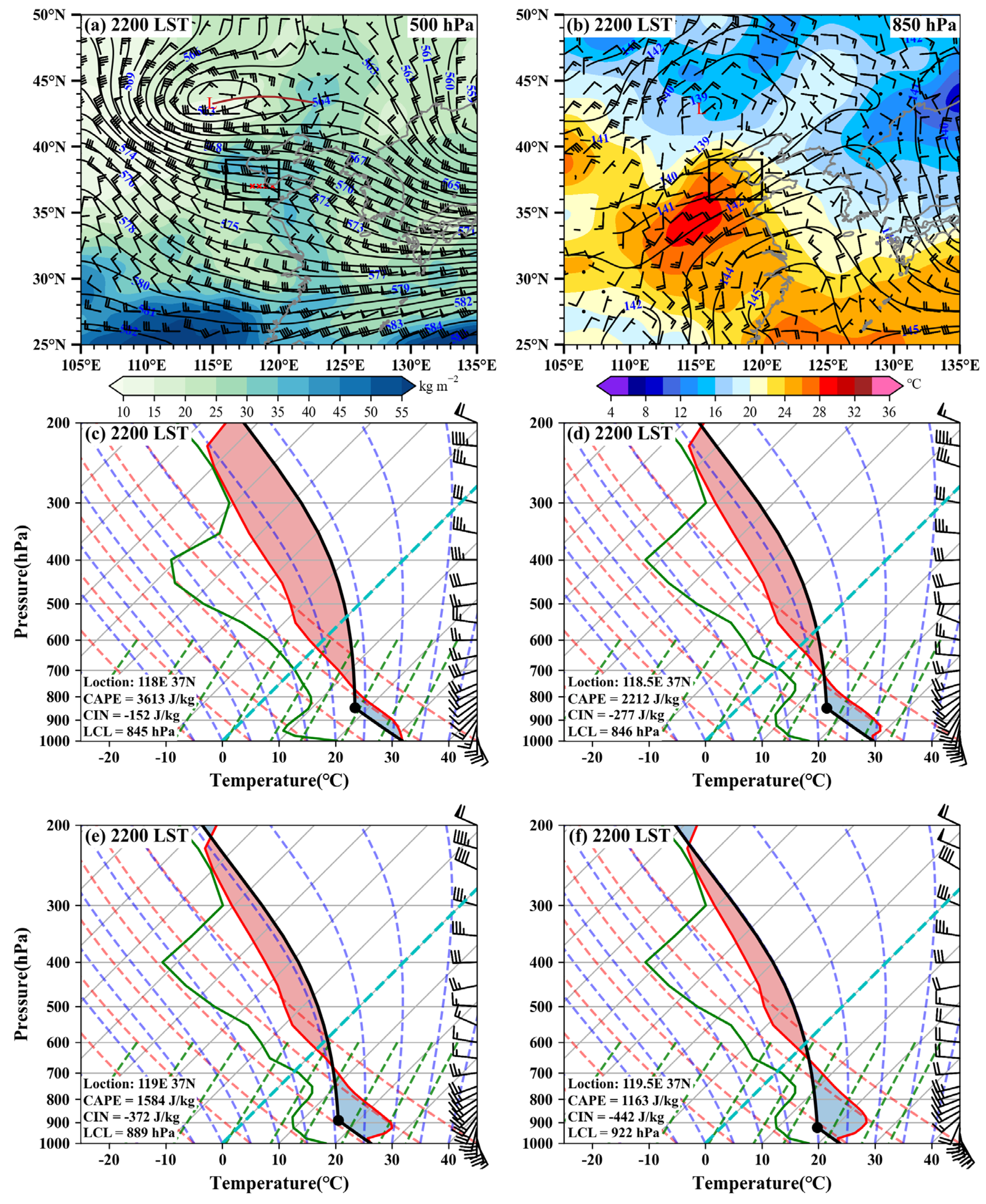
The vertical profiles (Figure 3c-f) provide insights into the atmospheric stratification before and after the passage of the SBF. Notably, significant convective available potential energy (CAPE), exceeding 1000 J kg⁻¹, is evident in all positions, highlighting the potential for conducive convective activity. Unexpectedly, the atmospheric boundary layer before SBF approaching is well-mixed (Figure 3c), indicating suboptimal conditions for bore formation prior to the GF-SBF collision. However, the approaching SBF from the coastline gradually stabilized boundary layer, leading to the formation of a pronounced inversion layer accompanied by increasing CIN. Consequently, in the SBF-governed environment, the initiation of deep convection is likely to occur if air parcels are lifted to the LFC. Furthermore, a gradual decrease in the lifting condensation level (LCL) from west to east indicates an increase in low-level water vapor content while the vertical wind profiles highlight the sea-land breeze circulation, consistent with observations.
3. Numerical Simulation
3.1. Experiment Design
Utilizing the WRF-ARW model [36], a high-resolution numerical simulation focusing on the collision between the MCS-generated GF and the coastal SBF, was conducted to explore the dynamics of bore. Numerical, in contrast to observational data, provide enhanced spatial and temporal, thereby offering a more detailed insight into the MCS evolution and the processes driving bore formation. The simulation started at 1000 LST on June 12, 2018, and lasted for 30 hours, employing a dual-layer, bidirectionally nested grid with of 3 km and 1 km (Figure 4). To analyze bore formation and its impact on the MCS, outputs were generated at 60-minute intervals for the outer layer and at one-minute intervals for the inner layer. Initial and boundary were derived from the European Centre for Medium-Range Weather Forecasts (ECMWF) data (Catalogue — Climate Data Store (copernicus.eu)). Table 1 outlines the specific details of the model.
3.2. Evaluation of the Model Simulation
Figure 5 illustrates the simulated composite reflectivity of the MCS and vertical velocity at 500 m above ground level (AGL). A comparative analysis between Figure 5d-i and Figure 1 demonstrates that the simulation successfully captures the structural evolution of the MCS. Specifically, the simulation effectively depicts the transformation of the MCS reflectivity core (≥45 dBZ) from a north-south linear to a bowed structure, eventually resembling a T-shaped convective system. As shown in Figure 5, the simulation accurately recreates the GF at the leading edge of the MCS, the SBF along the parallel coast, the ongoing collision between the GF and the SBF that formed undular bores and the development of nascent convection upstream the bore. However, the simulated MCS deviated about 100 km eastward, with an extensive region of weaker echoes on the system's western side. Such discrepancies are common in numerical simulations. [47,48,49].
Turn our attention to the evolution of the bore. At 1930 LST (Figure 5a), a narrow band of upward velocities, indicative of the GF, is observed along the southwestern leading edge of the MCS. As the GF collides with the SBF (Figure 5a and Figure 5b), this single band of uplift evolves into multiple bands. These bands of rising velocities gradually migrate from the MCS's leading edge, propagating southeastward and marking the formation of an undular bore (Figure 5c). This phenomenon favors the development of multiple convective cells upstream during its propagation (Figure 5c, d). Overall, the bore gradually intensified following its formation (Figure 5b-f), as indicated by a steady increase in its horizontal extension (Figure 5b-f) until 0310 LST, when the bore began to weaken (Figure 5g, h) and eventual dissipated (Figure 5i). The bore lasted approximately 6 hours, with its evolution closely linked to the intensification and extension of the MCS. Notably, the simulated collision between the GF and SBF occurred about 3 hours earlier than observed, resulting the bore's formation being similarly advanced in the simulation.
The simulation also recreates the critical process of destabilizing boundary layer caused by the approaching SBF, which plays a key role in bore formation (Figure 6). Under the influence of the SBF, the boundary layer gradually transitions from a mixed layer inland to a more stable layer closer to the coastline, marked by a decrease in CAPE and an increase in CIN (Figure 6c, d).
The following section will explore the dynamical mechanisms of the bore formed from the collision and bore’s role in CIs upstream.
4. Dynamic and Thermodynamic Structures of Bore formation and Its Role on CI
4.1. Horizontal Pattern
Figure 7 presents the simulated divergence field of 10 m horizontal wind, providing insight into the formation and evolution of the bore. Initially, a distinct and narrow convergence line marks the leading edge of the GF, while the SBF exhibited a primary structure aligned parallel to the coastline. They together formed an inverted V-shape (Figure 7a). At 1930 LST, the main bodies of GF and SBF had not yet to collided until 2000 LST (Figure 7b), the GF began colliding with the SBF from north to south, leading to a significant enhancement of convergence near the collision point. During the collision (Figure 7c, d), the strong convergence band associated with the GF becomes disturbed, with second and third convergence bands forming sequentially upstream, indicative of the formation of bore. By 2210 LST (Figure 7e), alternating bands of convergence and divergence appeared, signifying the development of the undular bore. The undular bore continues to propagate at a slightly higher speed than the MCS and initiates convective cells upstream (Figure 7f).
4.2. Dynamic and Thermodynamic Processes of Bore Formation
The vertical profiles of potential temperature (Figure 8) and vertical velocity (Figure 9) along the bore path offer a comprehensive perspective on the dynamics and thermodynamics involved in bore formation during the collision. At 1930 LST (Figure 8a1), before the collision begins, the GF was marked by an evident upward velocity band and the cold air trailing the GF was maintained by strong convective downdrafts originating from the mid-levels of the MCS and potentially enhanced by the nearby mountain range (Figure 8a1, Figure 9a1). By 2000 LST, the GF collided with the SBF (Figure 8a2) at its forefront, where convergence from the collision generated a strong updraft extending up to 5 km in depth (Figure 9a2). At 2040 LST, the continuous collision resulted in the formation of a "hump" downstream of the GF at 115.8°E, indicating the generation of a non-undular bore ahead of the GF or the beginning of the GF’s transformation into a gravity wave (Figure 8a3, Figure 9a3).
At the following times (Figure 8b, Figure 9b), due to being farther from the parent MCS and mountain range, the feed flow of the GF generally weakened and dissipated, meanwhile, the single “hump” downstream developed into multiple humps, indicating the transition from a non-undular bore to an undular bore. This transition is also evident in vertical velocity profiles, which shows a shift from a single to multiple bands of ascent (Figure 9b2). The undular bore propagated forward, with strongest uplifting reaching up to 5 km, comparable in strength to the upward motion at the front of the convective downdraft (Figure 9b2, 3).
4.3. Role of the Undular Bore on the CI
Convective cells are observed to initiate upstream of the undular bore as it propagates (Figure 5c, d). Figure 10 illustrates how the bore, along with its surrounding atmospheric conditions, facilitates CI along its trajectory.
In the southeastern region of the MCS, there is a substantial concentration of CAPE, especially behind the SBF, where CAPE is maximized and carried along by the SB. The collision between the GF and SBF induces significant uplift, transporting CAPE into the MCS and supporting its intensification (Figure 10a). When the undular bore forms, it propagates within favorable trapping layers associated with the SB, further promoting CI (Figure 10b). In particular, substantial CAPE-rich air parcels within the (SBL) are lifted, fueling the MCS and fostering the initiation of elevated convection. This process persists despite the reduction of CAPE due to radiative cooling, thereby sustaining the MCS's intensity and longevity. Additionally, the bore's progression diminishes CIN within the SBL, allowing the release of air parcels and facilitating CI (not given).
5. Dynamics Governing of Bore Formation
5.1. Classic Hydraulic Theory: Physical Mechanism of Bore Formation
The above analyses emphasize the dynamic and thermodynamic characteristics of the bore formation process, as well as the structure of the MCS, which are significantly influenced by the presence of the bore. To gain insight into the dynamics of bore formation, the classic hydraulic theory outlined by Rottman and Simpson (1989) [34] is applied, which has been widely adopted to explore the interactions between convective outflows and the SBL [2,7,22,24]. This theoretical framework considers a two-layer system of inviscid fluids interacting with an obstacle. In this framework, the Froude number () and dimensionless depth () serve as pivotal parameters delineating four distinct flow regimes: supercritical, partially obstructed, fully obstructed, and subcritical (Figure 11). Notably, the partially obstructed regime is particularly conducive to the generation of undular bores. The classification of these flow regimes is determined by the following equations:
where, , also referred to as bore strength, as mentioned in the introduction, is used to categorize the bores into three types: Type A (), Type B (), and Type C (). is given by:
where represents the depth of the cold pool and is the depth of the SBL, defined as the height at which the vertical gradient of potential temperature () is reduced to 0.005 K m-1, above which ambient conditions are typically mixed. The relevant equations to Froude number () are provided below:
In Equations (3) and (4), is velocity of the cold pool propagation, and is the average environmental velocity within the SBL. is gravitational acceleration, represents the virtual potential temperature near the surface within the SBL, and denotes the difference between the virtual potential temperature at the top of the SBL and near the surface. characterizes gravity wave velocity, which increases with the strength of the SBL.
By applying equations (2–4), the formation of disturbances is calculated during the specified timeframe (2000 LST-2210 LST; Figure 11). The results reveal that the disturbances arising from both the just-collision and post-collision ambient conditions are situated within region #2, a zone consistently conducive to the generation of undular bores. Table 2 provides a detailed summary of our calculations. Specifically, at the initial collision of the GF with the SBF, the is 400 m, subsequently increasing to approximately 550 m. As the bore evolves and the MCS intensifies, the gradually increases from 900 m to 1200 m. Given the variation of relative to , the , which aligns with the typical characteristics of Type A and B bores. The at 2000 LST, just-collision, is initially high at 1.97 due to a relatively low . However, as radiative cooling and the cooling effect of the SB, gradually decreases to approximately 1.3. Notably, while the remains relatively constant, the increases, leading to a corresponding rise in . By 2210 LST, the undular bore is well developed, and the mixing of cold pools from the GF and SBF results in substantial forward expansion. This expansion leads to a sudden increase in to 1.76 due to the significant enhancement of the .
5.2. Role of the Strong Convective Downdraft in Bore Formation
The results show that GF from the convective downdraft collided with the SBF, transitioning from a density current to a non-undular bore, and eventually to an undular one. In this process, the convective downdraft acts as the cold pool, a phenomenon documented in previous studies over China [22,24]. Studies have also highlighted that atmospheric density currents, often referred to as gravity currents in dynamic studies, are more sensitive to stratification, vertical wind shear, latent heat release, and evaporative cooling than their laboratory counterparts [50]. Therefore, analysis in this section will follow previous studies to better understand the mechanisms of the bore formation.
Haase and Smith (1989) [51] introduced the parameter to elucidate the influence of ambient stability, wind, and cold pools on the characteristics and evolution of gravity flows. The parameter , which is defined as the ratio of the SBL's strength to the incoming flow's strength is expressed as:
In Equation (5), represents the phase velocity of infinitesimal amplitude long waves in the SBL, characterizing the strength of the SBL. Meanwhile, denotes the propagation velocity of gravity waves in the absence of a SBL, characterizing the strength of the incoming flow. The related equations are as follows:
where is the Brunt-Väisälä frequency and is the total ambient density. They demonstrated that when < 0.7, the leading head or "hump" of the gravity flow becomes separate from the cold-air supply as the phase speed increases. However, it continues to move with the gravity flow as a perturbation resembling a large-amplitude solitary wave. At large Froude number ( = 1.13), the leading head may develop into multiple fluctuations, forming a wave-like disturbance. Similarly, Liu and Moncrieff (2000) [52] demonstrated that stratification significantly influence the structure of gravity flows. As the increases from a weak stratification of 0.004 s-1 to a strong one of 0.016 s-1, the gravity current transitions from a shallow body with an uplifted head to a structure featuring multiple heads. In this scenario, the leading head periodically dissipates while new heads form, indicating the formation of a wave-like disturbance.
In light of these studies, the environmental conditions are analyzed at 2000 LST. The results, with = 0.036 s-1, = 9.17 m s-1, = 17.88 m s-1, and = 0.51, suggest that the strong convective downdraft, upon colliding with the SBF, will promote the formation of an unsteady gravity current accompanied by wave-like disturbances. The results of the theoretical analysis further support the model-based observations of the separation and the periodic dissipation of the leading head of the gravity flow (mesoscale downdraft), as shown in Figure 8.
5.3. Waveguide Effect of LLJ
The CI within the MCS is facilitated by the prolonged persistence of the bore. Thus, this section will examine whether the ambient conditions support the long-lived bores.
As mentioned in the introduction, the key to sustaining bores as gravity disturbances lie in preventing the vertical propagation of fluctuating energy, thereby allowing the fluctuations to propagate horizontally. Crook (1988) [6] found that if the atmospheric boundary layer's stability and vertical wind profiles meet certain criteria, the Scorer parameter () will exhibit a steep gradient due to increased low-level wind speeds. Vertical fluctuations can be trapped when transitions from positive to negative with height. The is expressed as:
where the first term denotes the static stability associated and the second term denotes the horizontal wind curvature, is the ambient wind speed in the direction of bore motion, and is the mean velocity of the bore.
Using the theoretical framework, is calculated for 2210 LST to assess whether the post-formation environmental conditions favored the maintenance of the undular bore. The vertical distribution of , depicted in Figure 12, shows a steep decrease from large positive to negative values within the 300-600 m AGL range, before reverting to positive values above 600 m. This pattern suggests the presence of waveguide effects in the lower atmospheric layers. Martin and Johnson (2008) indicated that significant decreases in might be associated with subtle variations in wind profile curvature [31]. It is also evident in this case that the horizontal wind curvature term associated with the LLJ is the primary factor driving the transition from positive to negative . The results shown by Figure 12 are consistent with the evolution of the LLJ shown in Figure 7, where a wind component of the LLJ consistently opposes the direction of the bore.
6. Summary and Discussion
During the night of June 12 and the early hours of June 13, 2018, an MCS was observed by CZ and QD radar as it evolved and propagated southeastward into the western Bohai Sea. Ground-based observations, including the radars, confirmed the presence of a GF along the MCS’s convective outflow boundary, and a SBF located parallel to the coastline. As the MCS propagated southeastward, the GF collided with the SBF for approximately 1.5 hours. This continuous collision led to a rapid development of the MCS, characterized by a transformation in its reflectivity core, which initially displayed a linear north-south pattern, and then evolved into a distinct bow structure. Simultaneously, the collision caused the GF to transform into a non-undular bore, and later an undular one. Interestingly, before the collision, the SBL was well-mixed, which is typically considered unfavorable for bore formation. The undular bore then propagates with several convective cells initiated upstream.
The WRF-ARW model was employed to explore the collision dynamics between the GF and SBF, shedding light on the physical mechanisms driving bore generation and their impacts on convective processes. Results indicate that the atmospheric bore formed as a result of the collision between GF and SBF. In this case, the approaching SB establishes a SBL into which the GF from the convective downdraft intrudes, transitioning from a density current to a non-undular bore, and eventually to an undular one. Topography-induced downslope effects may also enhance the convective outflows, facilitating their collision. After the collision, the feeder flow of the GF weakened and dissipated, while the undular bore propagated forward along the top of SB, which acted as a wave duct. The dynamics governing this bore formation process are also investigated and validated using laboratory model theories.
Our findings also underscore that the MCS structure is significantly influenced by the undular bore. To the southeast of the MCS, the environment is characterized by a substantial amount of CAPE, particularly within the SBL. The bore propagated on the top of the SBL, lifting CAPE-rich air parcels that were continuously fed into the MCS, initiating multiple convective cells upstream of the bore. This process played a critical role in sustaining the intensity and longevity of the MCS.
In the eastern coast regions of China, MCSs associated GFs and SBs are prevalent during the warm season. Their collisions create a high likelihood of bore formation, regardless of the environmental boundary layer conditions. Understanding how density current collisions lead to bores formation and their impact on CI in unstable boundary layer conditions is crucial, especially for MCS that cause severe weathers during the daytime [53]. Our study investigates the mechanism of bore generation by density current collisions for the first time in China, highlighting that this may represent a novel mechanism for initiating intense convection along the China coast. The conceptual diagram in Figure 13 illustrates the formation and evolution of atmospheric bores and their roles in the initiation and maintenance of MCS.
Author Contributions
Conceptualization, S.Z. and X.X.; methodology, S.Z.; software, L.H.; validation, S.Z. and X.X.; formal analysis, L.H. and S.Z.; investigation, L.H., S.Z. and X.X.; resources, S.Z. and X.X.; data curation, L.H., S.Z. and X.X.; writing—original draft preparation, L.H.; writing—review and editing, S.Z.; visualization, L.H. and S.Z.; supervision, S.Z., X.X., H.H. and F.X.; project administration, S.Z. and X.X.; funding acquisition, S.Z., X.X., H.H. and F.X. All authors have read and agreed to the published version of the manuscript.
Funding
This work was supported by the National Key Research and Development Program of China (2023YFC3007502), Open Project of the High Impact Weather Key Laboratory of CMA, National Natural Science Foundation of China (42105007, 42005009, 42475009), and the Basic Research Fund of CAMS (2021Y016, 2021Z003).
Data Availability Statement
The ERA5 reanalysis data can be freely downloaded (available at https://doi.org/10.24381/cds.adbb2d47). The data used in this study are large and only the core datasets (including the radar data and WRF simulated data) have been uploaded to https://doi.org/10.6084/m9.figshare.27935634. Supplementary data is accessible through contacting the author.
Acknowledgments
The authors thank Nanjing University for supporting the study, where the high-resolution numerical simulations were performed on the supercomputer in the School of Atmospheric Sciences.
Conflicts of Interest
The authors declare no conflicts of interest.
References
- Knupp, K. Observational Analysis of a Gust Front to Bore to Solitary Wave Transition within an Evolving Nocturnal Boundary Layer. J. Atmos. Sci. 2006, 63, 2016–2035. [CrossRef]
- Haghi, K.R.; Parsons, D.B.; Shapiro, A. Bores Observed during IHOP_2002: The Relationship of Bores to the Nocturnal Environment. Mon. Wea. Rev. 2017, 145, 3929–3946. [CrossRef]
- Davies, L.; Reeder, M.J.; Lane, T.P. A climatology of atmospheric pressure jumps over southeastern Australia. Quart. J. Roy. Meteor. Soc. 2017, 143, 439-449. [CrossRef]
- Simpson, J.E. Gravity Currents: In the Environment and the Laboratory, 2d ed; Cambridge University Press, 1997; pp. 244. [CrossRef]
- Clarke, R.H. The morning glory: An atmospheric hydraulic jump. J. Appl. Meteor. 1972, 11, 304–311. [CrossRef]
- Crook, N.A. Trapping of low-level internal gravity-waves. J. Atmos. Sci. 1988, 45, 1533–1541. [CrossRef]
- Haghi, K.R.; Geerts, B.; Chipilski, H.G.; Johnson, A.; Degelia, S.; Imy, D.; Parsons, D.B.; Adams-Selin, R.D.; Turner, D.D.; Wang, X. Bore-ing into nocturnal convection. Bull. Amer. Meteor. Soc. 2019, 100, 1103–1121. [CrossRef]
- Clarke, R.H. Fair weather nocturnal inland wind surges and atmospheric bores. Part II: internal atmospheric bores in northern Australia. Aust. Meteor. Mag. 1983, 31, 147–160.
- Clarke, R.H. Colliding sea-breezes and the creation of internal atmospheric bore waves: Two-dimensional numerical studies. Aust. Meteor. Mag. 1984, 32, 207–226.
- Smith, R.K. Evening glory wave-cloud lines in northwestern Australia. Aust. Meteor. Mag. 1986, 34, 27–33.
- Noonan, J.A.; Smith, R.K. Sea-Breeze Circulations over Cape York Peninsula and the Generation of Gulf of Carpentaria Cloud Line Disturbances. J. Atmos. Sci. 1986, 43, 1679–1693. [CrossRef]
- Noonan, J.A.; Smith, R.K. The generation of North Australian cloud lines and the morning glory. Aust. Meteor. Mag. 1987, 35, 31–45.
- Wakimoto, R.M.; Kingsmill, D.E. Structure of an Atmospheric Undular Bore Generated from Colliding Boundaries during CaPE. Mon. Wea. Rev. 1995, 123, 1374–1393. [CrossRef]
- Kingsmill, D.E.; Crook N.A. An Observational Study of Atmospheric Bore Formation from Colliding Density Currents. Mon. Wea. Rev. 2003, 131, 2985–3002. [CrossRef]
- Karan, H.; Knupp, K. Radar and Profiler Analysis of Colliding Boundaries: A Case Study. Mon. Wea. Rev. 2009, 137, 2203–2222. [CrossRef]
- Lin, G.; Grasmick, C.; Geerts, B.; Wang, Z.; Deng, M. Convection Initiation and Bore Formation Following the Collision of Mesoscale Boundaries over a Developing Stable Boundary Layer: A Case Study from PECAN. Mon. Wea. Rev. 2021, 149, 2351–2367. [CrossRef]
- Koch, S.E.; Dorian, P.B.; Ferrare, R.; Melfi, S.H.; Skillman, W.C.; Whiteman, D. Structure of an Internal Bore and Dissipating Gravity Current as Revealed by Raman Lidar. Mon. Wea. Rev. 1991, 119, 857–887. [CrossRef]
- Koch, S.E.; Feltz, W.; Fabry, F.; Pagowski, M.; Geerts, B.; Bedka, K.M.; Miller, D.O.; Wilson, J.W. Turbulent Mixing Processes in Atmospheric Bores and Solitary Waves Deduced from Profiling Systems and Numerical Simulation. Mon. Wea. Rev. 2008, 136, 1373–1400. [CrossRef]
- Blake, B.T.; Parsons, D.B.; Haghi, K.R.; Castleberry, S.G. The Structure, Evolution, and Dynamics of a Nocturnal Convective System Simulated Using the WRF-ARW Model. Mon. Wea. Rev. 2017, 145, 3179–3201. [CrossRef]
- Grasmick, C.; Geerts, B.; Turner, D.D.; Wang, Z.; Weckwerth, T.M. The Relation between Nocturnal MCS Evolution and Its Outflow Boundaries in the Stable Boundary Layer: An Observational Study of the 15 July 2015 MCS in PECAN. Mon. Wea. Rev. 2018, 146, 3203–3226. [CrossRef]
- Loveless, D.M.; Wagner, T.J.; Turner, D.D.; Ackerman, S.A.; Feltz, W.F. A composite perspective on bore passages during the PECAN campaign. Mon. Wea. Rev. 2019, 147, 1395–1413. [CrossRef]
- Zhang, S.; Parsons, D.B.; Wang, Y. Wave Disturbances and Their Role in the Maintenance, Structure, and Evolution of a Mesoscale Convection System. J. Atmos. Sci. 2020, 77, 51–77. [CrossRef]
- Zhang, S.; Parsons, D.B.; Xu, X.; Wang, Y.; Liu, J.; Abulikemu, A.; Shen, W.; Zhang, X.; Zhang, S. A modeling study of an atmospheric bore associated with a nocturnal convective system over China. J. Geophys. Res. 2020, 125, e2019JD032279. [CrossRef]
- Zhang, S.; Parsons, D.B.; Xu, X.; Huang, H.; Xu, F.; Wu, T.; Chen, G.; Abulikemu, A.; Zhao, Y.; Zhang, S.; Tang, Y. The development of atmospheric bores in non-uniform baroclinic environments and their roles in the maintenance, structure, and evolution of an MCS. J. Geophys. Res. 2024, 129, e2023JD039319. [CrossRef]
- Mueller, D.; Geerts, B.; Wang, Z.; Deng, M.; Grasmick, C. Evolution and Vertical Structure of an Undular Bore Observed on 20 June 2015 during PECAN. Mon. Wea. Rev. 2017, 145, 3775–3794. [CrossRef]
- Weckwerth, T.M.; Hanesiak, J.; Wilson, J.W.; Trier, S.B.; Degelia, S.K.; Gallus, W.A.; Roberts R.D.; Wang, X. Nocturnal Convection Initiation during PECAN 2015. Bull. Amer. Meteor. Soc. 2019, 100, 2223-2239. [CrossRef]
- Scorer, R.S. Theory of waves in the lee of mountains. Quart. J. Roy. Meteor. Soc. 1949, 75, 41–56. [CrossRef]
- Haghi, K.R.; Durran, D.R. On the Dynamics of Atmospheric Bores. J. Atmos. Sci. 2021, 78, 313–327. [CrossRef]
- Parsons, D.B.; Haghi, K.R.; Halbert, K.T.; Elmer, B.; Wang, J. The potential role of atmospheric bores and gravity waves in the initiation and maintenance of nocturnal convection over the Southern Great Plains. J. Atmos. Sci. 2019, 76, 43–68. [CrossRef]
- Osborne, S.R.; Lapworth, A. Initiation and Propagation of an Atmospheric Bore in a Numerical Forecast Model: A Comparison with Observations. J. Appl. Meteor. Climatol. 2017, 56, 2999-3016. [CrossRef]
- Martin, E.R.; Johnson, R.H. An Observational and Modeling Study of an Atmospheric Internal Bore during NAME 2004. Mon. Wea. Rev. 2008, 136, 4150–4167. [CrossRef]
- Lombardo, K. Kumjian, M.R. Observations of the Discrete Propagation of a Mesoscale Convective System during RELAMPAGO–CACTI. Mon. Wea. Rev. 2022, 150, 2111–2138. [CrossRef]
- Zhang, S.; Parsons, D.B.; Xu, X.; Sun, J.; Wu, T.; Xu, F.; Wei, N.; Chen, G. Bores observed during the warm season of 2015–2019 over the southern North China Plain. Geophys. Res. Lett. 2022, 49, e2022GL099205. [CrossRef]
- Rottman, J.W.; Simpson, J.E. The formation of internal bores in the atmosphere: A laboratory model. Quart. J. Roy. Meteor. Soc. 1989, 115, 941–963. [CrossRef]
- Smith, R.K. Travelling waves and bores in the lower atmosphere: the 'morning glory' and related phenomena. Earth Sci. Rev. 1998, 25, 267-290. [CrossRef]
- Skamarock, W.; Klemp, J.; Dudhia, J.; Gill, D.O.; Liu, Z.; Berner, J.; Wang, W.; Powers, J.G.; Duda, M.G.; Barker, D.; Huang, X. A Description of the Advanced Research WRF Model Version 4.1. 2019. [CrossRef]
- Min, C.; Chen, S.; Gourley, J.J.; Chen, H.; Zhang, A.; Huang, Y.; Huang, C. Coverage of China New Generation Weather Radar Network. Adv. Meteorol. 2019, 2019, 1-10. [CrossRef]
- Huang, Y.; Meng, Z.; Li, W.; Bai, L.; Meng, X. General features of radar-observed boundary layer convergence lines and their associated convection over a sharp vegetation-contrast area. Geophys. Res. Lett. 2019, 46, 2865–2873. [CrossRef]
- Hersbach, H.; Bell, B.; Berrisford, P.; Biavati, G.; Horányi, A.; Muñoz Sabater, J.; Nicolas, J.; Peubey, C.; Radu, R.; Rozum, I.; Schepers, D.; Simmons, A.; Soci, C.; Dee, D.; Thépaut, J-N. ERA5 hourly data on single levels from 1940 to present [Dataset]. Copernicus Climate Change Service (C3S) Climate Data Store (CDS). 2023. [CrossRef]
- Thompson, G.; Field, P.R.; Rasmussen, R.M.; Hall, W.D. Explicit Forecasts of Winter Precipitation Using an Improved Bulk Microphysics Scheme. Part II: Implementation of a New Snow Parameterization. Mon. Wea. Rev. 2008, 136, 5095-5115. [CrossRef]
- Mlawer, E.J.; Taubman S.J.; Brown P.D.; Iacono M.J.; Clough, S.A. Radiative transfer for inhomogeneous atmospheres: RRTM, a validated correlated-k model for the longwave. J. Geophys. Res. 1997, 102, 16663-16682. [CrossRef]
- Dudhia, J. Numerical study of convection observed during the winter monsoon experiment using a mesoscale two-dimensional model. J. Atmos. Sci. 1989, 46, 3077-3107. [CrossRef]
- Janjic, Z. The surface layer in the NCEP Eta Model. Eleventh Conference on Numerical Weather Prediction, Norfolk, VA, 19-23 August 1996. Amer. Meteor. Soc., Boston, MA, 354-355.
- Chen, F.; Dudhia, J. Coupling an Advanced Land Surface–Hydrology Model with the Penn State–NCAR MM5 Modeling System. Part I: Model Implementation and Sensitivity. Mon. Wea. Rev. 2001, 129, 569-585. [CrossRef]
- Mellor, G.L.; Yamada T. Development of a turbulence closure model for geophysical fluid problems. Rev. Geophys. 1982, 20, 851-875. [CrossRef]
- Grell, G.A.; Dévényi D. A generalized approach to parameterizing convection combining ensemble and data assimilation techniques. Geophys. Res. Lett. 2002, 29. [CrossRef]
- Morrison, H.; Milbrandt, J.A. Parameterization of cloud microphysics based on the prediction of bulk ice particle properties. Part I: Scheme description and idealized tests. J. Atmos. Sci. 2015, 72, 287–311. [CrossRef]
- Wei, P.; Xu, X.; Xue, M.; Zhang, C.; Wang, Y.; Zhao, K.; Zhou, A.; Zhang, S.; Zhu, K. On the Key Dynamical Processes Supporting the 21.7 Zhengzhou Record-breaking Hourly Rainfall in China. Adv. Atmos. Sci. 2023, 40, 337–349. [CrossRef]
- Xu, X.; Ju, Y.; Liu. Q.; Zhao, K.; Xue, M.; Zhang, S.; Zhou, A.; Tang, Y. Dynamics of two episodes of high winds produced by an unusually long-lived quasi-linear convective system in South China. J. Atmos. Sci. 2024, 81, 1449-1473. [CrossRef]
- Haertel, P.T.; Johnson, R.H.; Tulich, S.N. Some simple simulations of thunderstorm outflows. J. Atmos. Sci. 2001, 58, 504–516. [CrossRef]
- Haase, S.P.; Smith, R.K. The numerical simulation of atmospheric gravity currents. Part II. Environments with stable layers. Geophys. Astrophys. Fluid Dyn. 1989, 46, 35–51. [CrossRef]
- Liu, C.; Moncrieff, M.W. Simulated density currents in idealized stratified environments. Mon. Wea. Rev. 2000, 128, 1420–1437. [CrossRef]
- Zhang, Q.; Ni, X.; Zhang, F. Decreasing trend in severe weather occurrence over China during the past 50 years. Sci. Rep. 2017, 7, 42310. [CrossRef]
Figure 1.
Radar reflectivity (shaded, units: dBZ) from the CZ and QD radar station at an elevation angle of 0.5° and observed surface wind fields (grey vectors, units: m s-1) from operational ground-based observation networks. The CZ radar was observed from 2200 LST on 12 June to 0000 LST on 13 June 2018, while and the QD radar was observed from 0031 LST on 13 June to 0231 LST on 13 June 2018. The red × in panel (a) indicates the sounding location in Figure 3, the black lozenges in panels (a) and (d) indicate the ground-based stations, the red dashed cycles in panels (c) and (d) indicate the CI of convective cell in RFL upstream, and the blue arrows in panels (e) and (f) indicate an undular bore. The light orange shading indicates terrain greater than 200 m above ground level (AGL). By integrating data from the ground-based network with radar imagery, the positions of the leading edge of MCS convective outflow (i.e., GF) and the SBF were indicated by black solid and purple solid curves, respectively. The solid black curve changes to a dashed black curve, indicating that the collision is in progress.
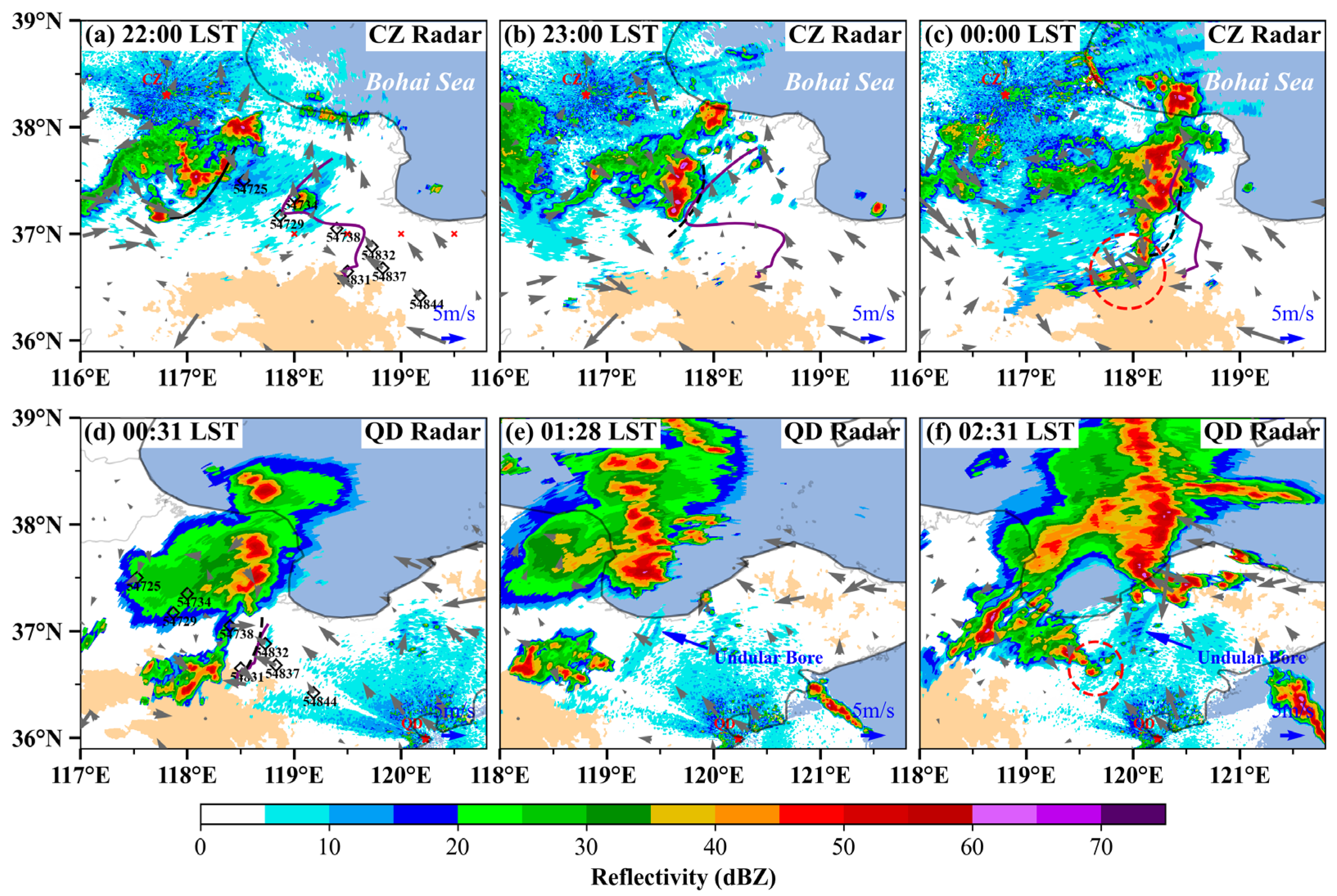
Figure 4.
Domain configurations utilized in the WRF Preprocessing System and simulations include an outer domain with a 3 km horizontal grid spacing, while the inner domain, labeled as d02, is represented by a box with a 1 km resolution.
Figure 4.
Domain configurations utilized in the WRF Preprocessing System and simulations include an outer domain with a 3 km horizontal grid spacing, while the inner domain, labeled as d02, is represented by a box with a 1 km resolution.
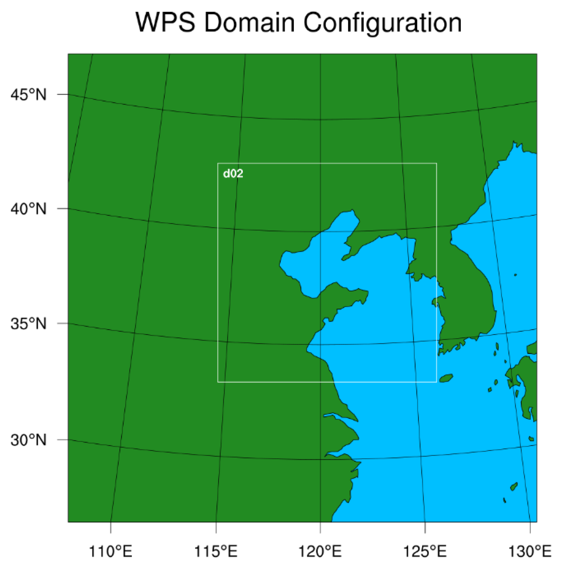
Figure 5.
Composite reflectivity (shaded, units: dBZ) and 10 m horizontal wind (grey vectors, units: m s-1) simulated by the WRF model at the 1-km resolution from 1930 LST on 12 June to 0440 LST on 13 June 2018. The red rectangle in panel (a) marks the sounding location shown in Figure 6. Thin black dashed contours in panels (a)-(c) indicate vertical velocities of 0.5 m s-1 at 500 m AGL, while thick black dashed contours in panels (d)-(i) indicate 1 m s-1 for clarity.
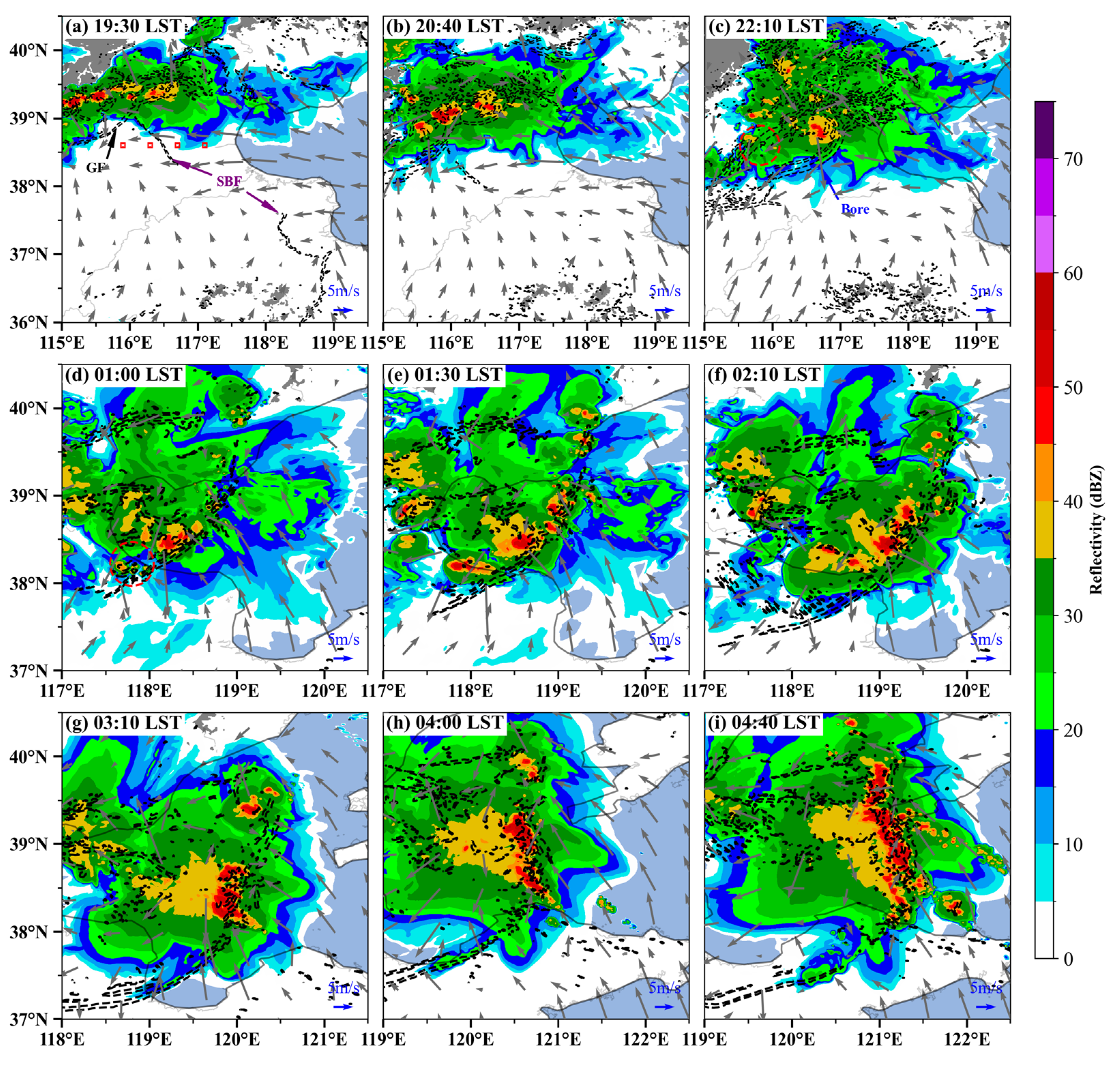
Figure 6.
Similar to Figure 3c-f, but showing simulated vertical profiles at 1930 LST from the areas marked by red rectangles in Figure 5a. Panels (a), (b), (c), and (d) correspond to the rectangles from west to east, respectively.
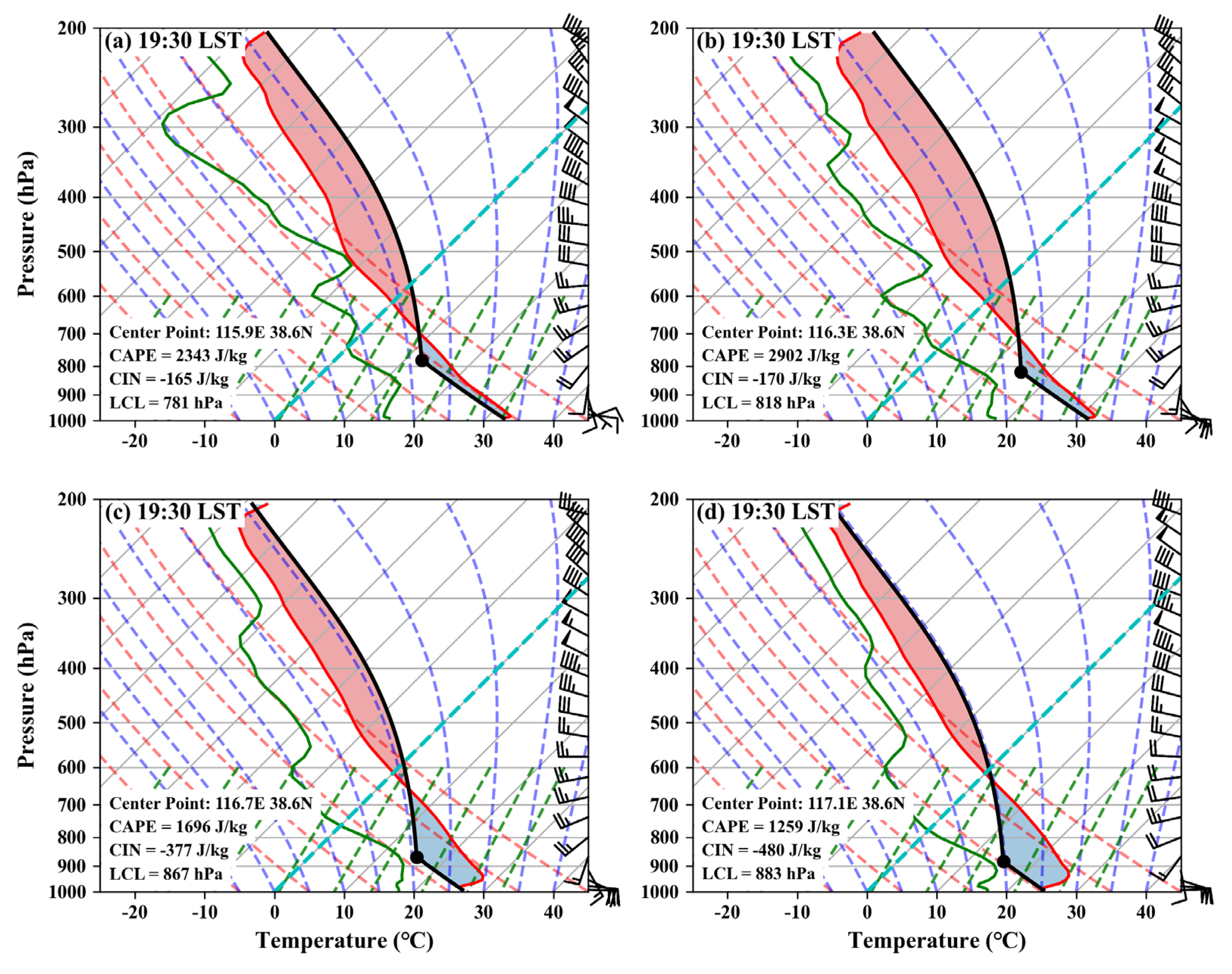
Figure 7.
Divergence (shaded, units: s-1) of 10 m horizontal wind, composite reflectivity of 35 dBZ (green contours), and horizontal wind (vectors, units: m s-1) at 1 km AGL simulated by the WRF model in the 1-km-resolution domain at (a) 1930, (b) 2000, (c) 2040, (d) 2120, (e) 2210, and (f) 2300 LST. The rectangles indicate collision regions between GF and SBF. The arrow labeled in panel (e) indicates the undular bore, while the red dashed cycle indicates the initiation of convective cells upstream of the undular bore. The blue dashed lines indicate the vertical cross-section location for Figure 8, Figure 9 and Figure 10.
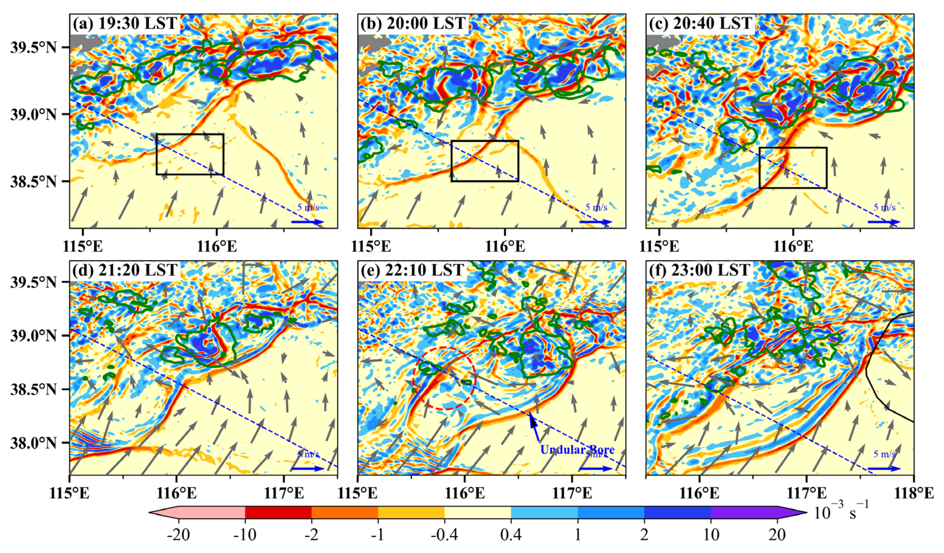
Figure 8.
Vertical cross sections of potential temperature (shaded, units: K) and ground-relative wind (vectors, units: m s-1) at (a1) 1930, (a2) 2000, (a3) 2040, (b1) 2120, (b2) 2210, and (b3) 2300 LST, along the blue dashed lines in Figure 7. The blue dashed and purple dashed lines in panel (a1) indicate the longitude of the leading edges of the GF and SBF, respectively. Green solid and dashed contours indicate the reflectivity of 35 dBZ and 15 dBZ, respectively. Vertical velocity is exaggerated 10 times for clarity. The translucent black curved arrows indicate the location of strong downdraft.
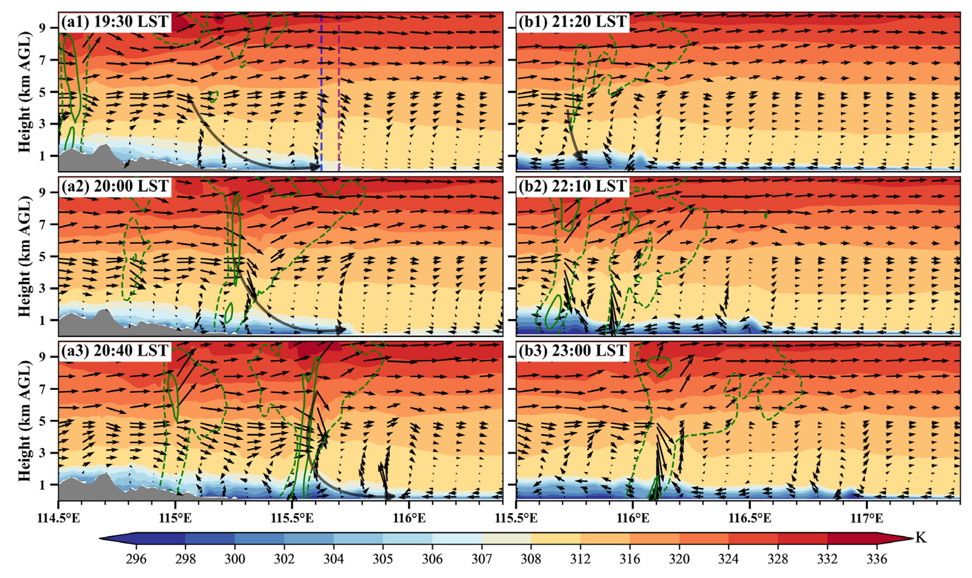
Figure 9.
Similar to Figure 8, but showing the vertical velocity (shaded, units: m s-1). The blue contours indicate potential temperature of 307 K.
Figure 9.
Similar to Figure 8, but showing the vertical velocity (shaded, units: m s-1). The blue contours indicate potential temperature of 307 K.
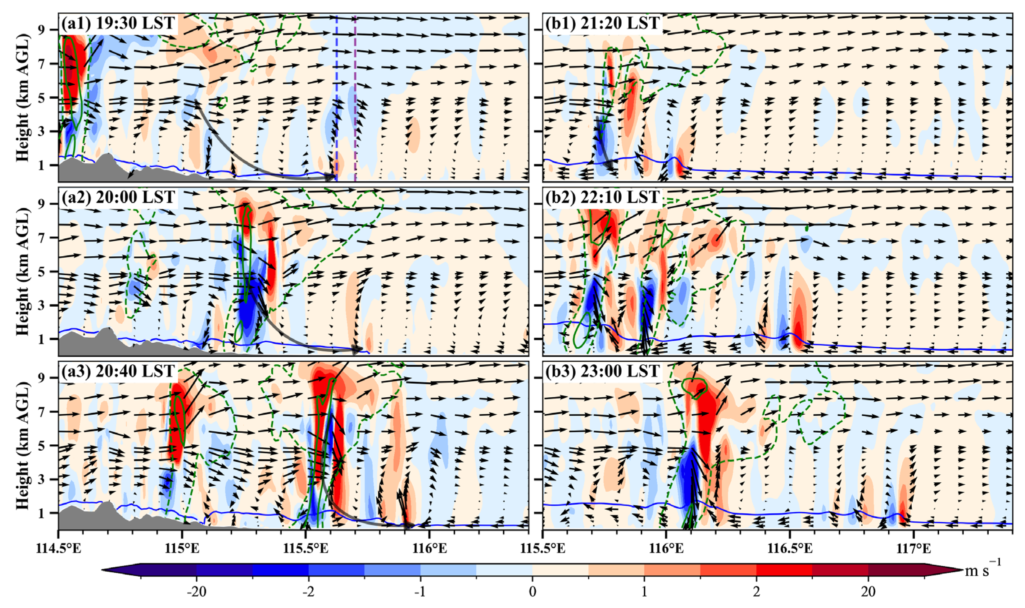
Figure 10.
Similar to Figure 9, but showing the CAPE (shaded, units: J kg-1). The translucent red curved arrows indicate the locations of the bore lifting.
Figure 10.
Similar to Figure 9, but showing the CAPE (shaded, units: J kg-1). The translucent red curved arrows indicate the locations of the bore lifting.
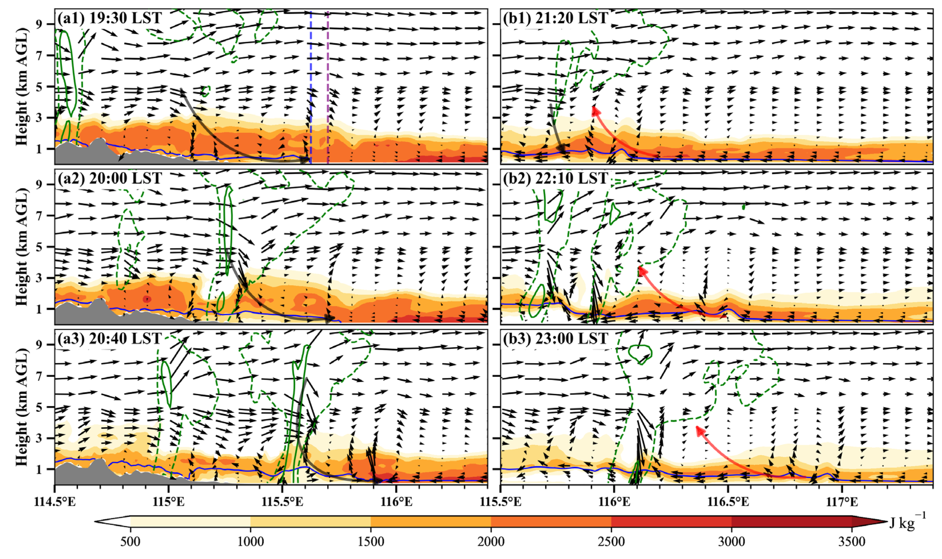
Figure 11.
The non-dimensional parameters and during the evolution of the bore. The two parameter spaces represent the predicted (#1) supercritical, (#2) partially blocked, (#3) completely blocked and (#4) subcritical flow regimes. Environmental estimates from the simulations are marked within this phase space: a black star for 2000 LST, a navy diamond for 2040 LST, a blue circle for 2120 LST, and a red circle for 2210 LST.
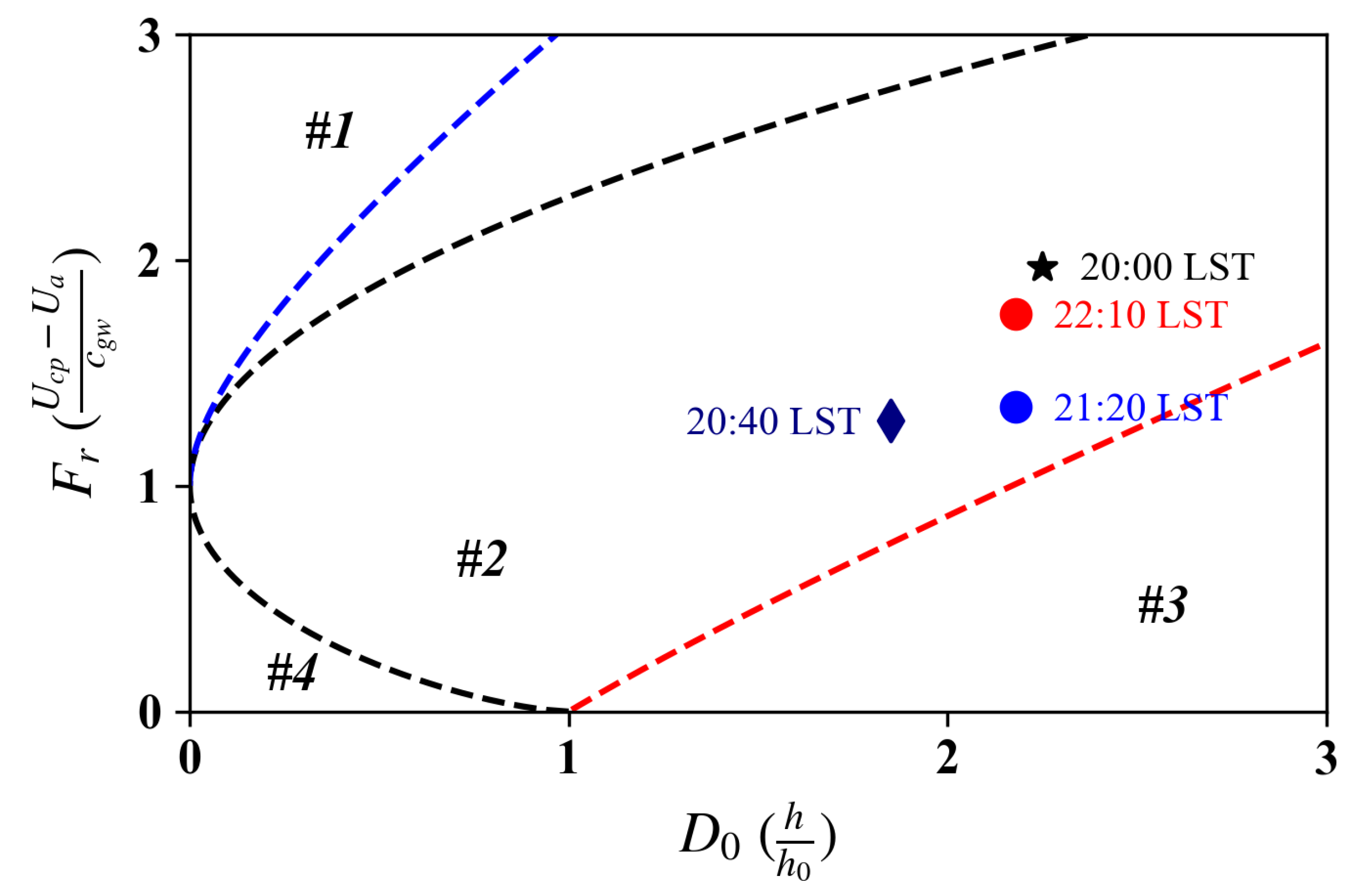
Figure 12.
Height profiles of the Scorer parameter (thick black lines, unit: 10-5 m-2), along with its components: static stability (blue lines) and curvature term (red lines), at 2210 LST in the southeastern portions of the cross-section shown in Figure 10b2.
Figure 12.
Height profiles of the Scorer parameter (thick black lines, unit: 10-5 m-2), along with its components: static stability (blue lines) and curvature term (red lines), at 2210 LST in the southeastern portions of the cross-section shown in Figure 10b2.
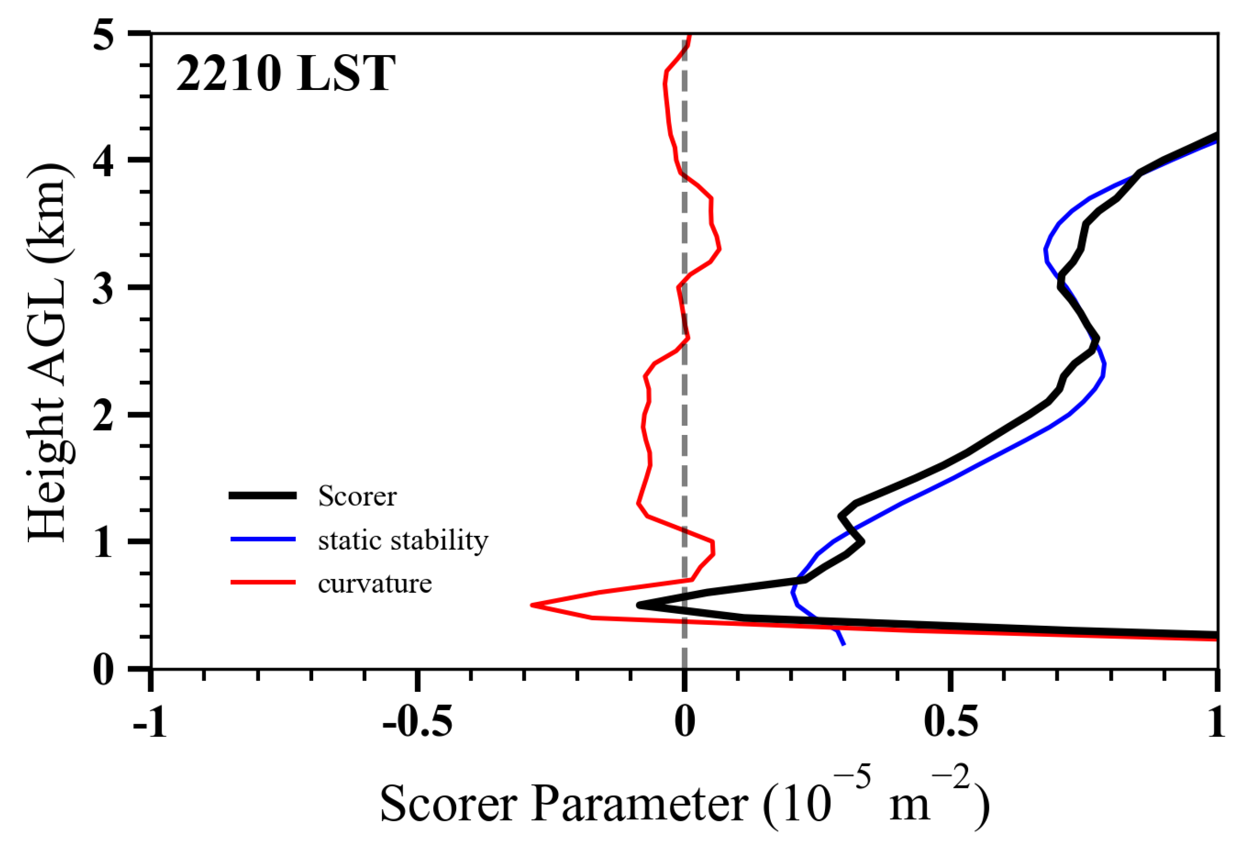
Figure 13.
Schematic of the collision between the convective outflow (shaded, emerald green) and the SBF (shaded, sky blue) in this case study, where depicts the pre-collision state (a), the collision itself (b), and the post-collision state (c). Translucent red arrows indicate the lifting resulting from collisions in panel (b), as well as the lifting from the bore in panel (c). The orange dots indicate unstable air parcels.
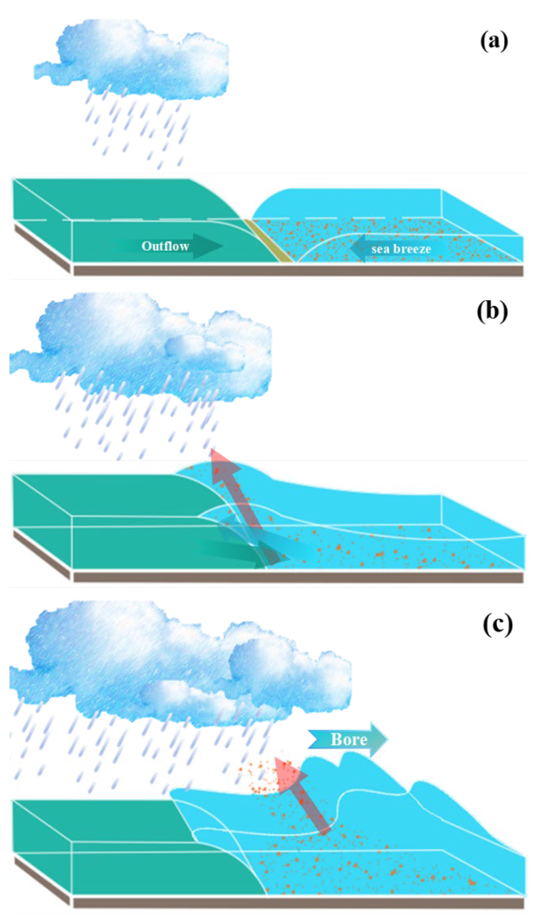

Table 1.
Summary of the ARW configuration for this study.
| Domain #1 | Domain #2 | References | |
|---|---|---|---|
| Grid Spacing | 3 km | 1 km | |
| Horizontal dimensions | 2247 km × 2247 km | 1050 km × 1050 km | |
| Vertical sigma levels | 45 | 45 | |
| Model top pressure | 200 hPa | 200 hPa | |
| ICs and LBCs | EAR5 reanalysis | EAR5 reanalysis | |
| Microphysics | Thompson | Thompson | Thompson et al. 2008 [40] |
| Longwave radiation | RRTM | RRTM | Mlawer et al. 1997 [41] |
| Shortwave radiation | Dudhia | Dudhia | Dudhia 1989 [42] |
| Surface layer | Monin–Obukhov–Janjic | Monin–Obukhov–Janjic | Janjic 1996 [43] |
| Land surface model | Noah | Noah | Chen and Dudhia 2001 [44] |
| Boundary layer physics | MYJ | MYJ | Mellor and Yamada 1982 [45] |
| Cumulus parameterization | Grell and Dévényi | Grell and Dévényi | Grell and Dévényi 2002 [46] |
Table 2.
Estimated variables, and values of and .
| 2000 LST | 2040 LST | 2120 LST | 2210 LST | |
|---|---|---|---|---|
| 400 | 540 | 550 | 550 | |
| 900 | 1000 | 1200 | 1200 | |
| 7.46 | 6.83 | 6.87 | 16.43 | |
| -8.64 | -8.51 | -9.88 | -7.99 | |
| 8.19 | 11.87 | 12.38 | 13.89 | |
| 1.97 | 1.29 | 1.35 | 1.76 | |
| 2.25 | 1.85 | 2.18 | 2.18 |
Disclaimer/Publisher’s Note: The statements, opinions and data contained in all publications are solely those of the individual author(s) and contributor(s) and not of MDPI and/or the editor(s). MDPI and/or the editor(s) disclaim responsibility for any injury to people or property resulting from any ideas, methods, instructions or products referred to in the content. |
© 2024 by the authors. Licensee MDPI, Basel, Switzerland. This article is an open access article distributed under the terms and conditions of the Creative Commons Attribution (CC BY) license (http://creativecommons.org/licenses/by/4.0/).
Copyright: This open access article is published under a Creative Commons CC BY 4.0 license, which permit the free download, distribution, and reuse, provided that the author and preprint are cited in any reuse.


