Preprint
Article

This version is not peer-reviewed.

Denoising X-ray Diffraction two-dimensional patterns by a Lattice Boltzmann Method

A peer-reviewed article of this preprint also exists.

Submitted:

12 December 2024

Posted:

13 December 2024

You are already at the latest version

Abstract

An X-ray Diffraction pattern consists of the relevant information (the signal) and the noisy background. Under the assumption that they behave as the components of a two-dimensional mixture (bicomponent fluid) having slightly different physical properties related to the density-gradients, a Lattice Boltzmann Method is applied to disentangle the two different diffusive dynamics. The solution is numerically stable, computationally not demanding and, moreover, it provides an efficient increase of the signal-to-noise ratio for patterns blurred by poissonian noise and affected by collection data anomalies (fiber-like samples, experimental setup, etc.). The model has been succesfully applied to different resolution images.

Keywords: 
;  ;  

1. Introduction

X-ray tomography is a versatile technique for investigating the internal structure of nano(bio)-materials with applications in energy research [1], life sciences [2], medicine [3,4,5] and many other fields, both at synchrotron radiation facilities and at microfocus laboratory sources [6].
In recent years, advancements in X-ray diffraction (XRD) image denoising have continued to evolve, driven by both traditional [7]1 and machine learning approaches, particularly (convolutional) neural networks and techniques alike [8,9,10].
In spite of the prominence recently gained by deep learning techniques, it is worth stressing that these models have to be trained on large datasets to learn to distinguish between noise and signal, and improving the clarity of XRD images. For instance, new benchmark datasets and evaluation metrics are being developed to standardize the assessment of denoising techniques and, to enhance model performance, researchers use data augmentation techniques: this involves artificially increasing the size of the training dataset through transformations like rotations, scaling, and noise addition, which helps in training more robust models [11]. On the other hand, the integration of advanced machine learning techniques with traditional denoising methods is significantly enhancing the quality of X-ray diffraction images, leading to more accurate analyses and interpretations in various scientific and industrial applications. This is particularly the case of real-time processing, where advances in hardware and software are making it feasible to perform denoising in real-time, which is particularly useful for high-throughput XRD applications. Also combining machine learning with traditional signal processing techniques is becoming more common (hybrid approaches). For example, pre-processing steps might use classical denoising methods, followed by machine learning techniques for further refinement.
Furthermore tackling the problem of image restoration solely from an algorithmic perspective may even include generative aspects, that can bias the ground truth: noise profiles are unknown and often include noise from multiple distinct sources, substantially reducing the applicability of simulation-based approaches. Therefore, techniques like wavelet transform and Physics inspired adaptive filtering are still being refined to handle varying types of noise and different XRD data characteristics. In order to accomplish the task of preserving important features while reducing noise, focusing on a genuinely Physics-grounded method is still worth.

2. A Fluidistic Approach

An XRD two-dimensional pattern is described as a fluid representing the signal and the noise; the denoising process can be thought of as the result of the motion of such a fluid towards a steady state (the original noisy image): due to internal friction (viscosity) and thermal conduction, the effect of energy dissipation, occurring during the motion of this fluid, on that motion itself, results in the thermodynamic irreversibility of the motion. The different diffusive dynamics of signal/noise finally smears the noise and this process is irreversible. In order to obtain the equations describing the motion of a viscous fluid, some terms must be added to the Euler’s equations modelling an ideal fluid.
The Navier–Stokes equations are fundamental mathematical equations in fluid mechanics that describe the motion of viscous fluid substances. They are derived from the principles of conservation of mass, momentum, and energy. These nonlinear partial differential equations account for various factors, including pressure, velocity, and external forces, making them essential for understanding fluid behavior in diverse applications, from weather patterns to aerospace engineering. Solving the Navier–Stokes equations provides insights into complex fluid dynamics, although they are known for their mathematical challenges and are central to the unsolved problem of turbulence in fluid flow [12].
The diffusion equation and the Navier-Stokes equations are both fundamental in fluid dynamics but describe different physical phenomena.
  • Diffusion Equation. This equation models the process of substance spreading due to concentration gradients. It is typically written as c t = D 2 c , where c is the concentration of the substance, D is the diffusion coefficient, and 2 is the Laplacian operator. It captures how substances diffuse through a medium over time.
  • Navier–Stokes Equations. These equations describe the motion of fluid substances and account for viscosity and external forces. They can be expressed as:
    u t + ( u · ) u = 1 ρ p + ν 2 u + f , where u is the fluid velocity, p is the pressure, ν is the kinematic viscosity, ρ is the density, and f represents external forces.
There are relationships between the two equations, namely viscous effects, transport phenomena and limits. Indeed, the diffusion equation can be seen as a simplified version of the Navier–Stokes equations when considering mass transport in a viscous fluid. In this context, the term representing diffusion can be derived from the viscous effects of the fluid motion. Furthermore, the Navier–Stokes equations govern fluid flow, while the diffusion equation describes how quantities like temperature, concentration, or species disperse within that flow2. Finally in low Reynolds number flows (where inertial forces are negligible compared to viscous forces), the Navier–Stokes equations can approximate diffusion-like behavior.
In summary, while both equations are foundational to understanding fluid behavior, the diffusion equation focuses on concentration changes, whereas the Navier–Stokes equations address the overall dynamics of fluid motion.

2.1. A Navier–Stokes Inspired Model

In the Field Theory, the relevant functions (i.e. Lagrangian L and Hamiltonian H densities) to describe the model of a dynamical field (u), having a mass ( w 1 ) and interacting with an external field ( ρ ), read:
L = d e f . ı 2 u t u t u u α β | u ρ | 2 +
+ w u · u + λ 2 w ln w ; H = d e f . Π t u + Π t u L Π ( ) = d e f . L t u ( ) = ı 2 u ( ) =
= α β | u ρ | 2 + w u · u + λ 2 w ln w .
The model time evolution follows from the minimization of the functionals energy ( E ) and action ( S ):
E u ( ) , u ( ) , w = d 2 x H u ( ) , u ( ) , w ,
S u ( ) , u ( ) , w = d t d 2 x L u ( ) , u ( ) , w ,
where the functional dependence on the dynamical fields u ( ) (together with their conjugate momentum densities, u ( ) ) and on the non-dynamical3 field w is made explicit.
Finally the equations of motion for the field(s) promptly read:
δ S = 0 τ = ı t τ u ( ) = α β ( ρ u ( ) ) + + w u ( ) , w = 1 + u · u λ 2 1 ,
where the boxed expressions represent the density (e.g. XRD image) gradient-dependent diffusive term. While this approach has been fruitfully applied to the subject in the past [7], its feasibility is undermined by the difficulty in separating the different time-scales, in particular the collision time-scale and the propagating one.

2.2. Lattice Boltzmann Method: Overview

The Lattice Boltzmann Methods (LBM) is a numerical approach used to simulate fluid dynamics [13,14,15]. Unlike traditional methods like the Navier–Stokes equations, LBM models fluid flow by simulating the movement of particles on a discrete lattice grid as follows.
  • Discrete Lattice. The fluid is represented by particles moving on a fixed grid with discrete directions: the lattice dimensions (D) and the neighborhood (Q, the number of nearest neighbors, including the site itself) define the particular lattice Boltzmann method: e.g. D2Q9 means nine nearest neighbors for each site on a two-dimensional lattice · .
  • Collision Step. Particles collide and exchange momentum according to probabilistic rules.
  • Streaming Step. After collisions, particles move to neighboring lattice sites.
  • Macroscopic Variables. From the particle distribution functions, macroscopic quantities like density and velocity are computed.
While LBM is particularly useful for complex boundary conditions and multiphase flows due to its straightforward implementation and ability to handle irregular geometries, this method allows for better handling of noise at different scales by adapting to varying noise levels across the two-dimensional X-ray patterns.

2.3. Lattice Boltzmann Method: Application

Due to the equivalence between the hydrodynamic model (transport equation) and the fluid-mechanics (Hamiltonian), an approach is explored where the two dynamics can be explicitly and straightforwardly disentangled. In the hydrodynamic model, indeed, the (microscopic) distribution f = f ( t , x , p ) satisfies the Boltzmann transport equation d f d τ = C [ f ] , where the total time derivative reads d ( · ) d t = ( · ) t + x · · x + p · · p , while C [ f ] is the collision integral accounting for the particle interactions4. The change to macroscopic equations is achieved by integrating out the degrees of freedom which are integrals of the motion between two collisions (in the absence of an external field), e.g.  u ( x , t ) = d 2 p f ( x , p , t ) .
According to the Hamilton’s equations [18] p · = F e x t , being the latter one the external force acting on the fluid particle (the two-dimensional X-ray pattern image pixel).
C [ f ] ω f f e q , f e q ( x , p ) = d e f . ρ ( x ) 2 π exp | p | 2 2 ,
where f e q satisfies the transport equation with F e x t = U and the external potential  U = ln ( ρ ) . The collision integral has been approximated by the Bhatnagar–Gross–Krook model [19], where the linear collision time-scale ( ω 1 ) has been spotted as the relaxation of the time dependent X-ray two-dimensional pattern f ( t , x , p ) to the constant noisy one f e q ( x , p ) ρ ( x ) . Such an evolution accounts for the different diffusion dynamics of noise/signal to improve the signal-to-noise ratio. The lattice (Boltzmann) method simulates the evolution through a cycle of propagation and collision on a regular lattice where the microscopic distribution function propagates to the nearest neighbor sites in precisely one time-step, once a suitable discrete momenta set has been chosen. By performing such a spatio-temporal discretization, the Boltzmann transport equation reads
f i ( x + p i δ t , t + δ t ) f i ( x , t ) = ω ˜ 1 f i ( x , t ) f e q i ( x ) ,
where ω ˜ 1 is the re-scaled relaxation time and the index i refers to the set of momenta p i chosen to connect the lattice sites5. The anisotropic diffusive term (the boxed expressions in Equation (5)) is added by hand. The algorithm straightforwardly follows: updating a few number of floating-point arithmetic operations is computationally not demanding and the task can be easily parallelized6.

3. Results and Conclusions

The only parameters that are left in the numerical solution of Equation (7) are α and β (the parameter λ , related to the non-dynamical field w, is proportional to the norm of the conjugate momentum density | u | and it adiabatically changes [21]). While α = 1 . 15 is the highest value that can be used to guarantee stability without slowing down the convergence when the method is applied to an image affected by a gaussian noise (e.g. the classical Lenna image of Figure 1), α = 0 . 85 appears to be the optimal solution for an application of the technique to the XRD two-dimensional patterns (e.g. Figure 2, Figure 3 and Figure 4). In fact, one has to balance between the need to use the highest possible value of ω ˜ 1 of the Equation (7) to reduce the number of iterations to achieve the final reconstructed image and the stability requirement that fixes an upper bound for ω ˜ 1 . The efficiency in image filtering is evaluated by measuring the peak-to-signal noise ratio (PSNR) defined as
PSNR = d e f . 20 log 10 | u ρ 0 | 2 max ( ρ 0 ) ,
where ρ 0 is the original image without noise and . . . denotes a sum over all the pixels of the images. This quantity is measured in decibels, and higher values correspond to a better denoising. The parameter β was varied in the method to obtain the highest possible values of PSNR.
Beside the gaussian-noise affected images, the XRD experimental setups collect data on two-dimensional arrays, where a Poisson counting statistics accordingly needs a noise reduction.
Wide Angle X-ray Diffraction (WAXD) patterns are used to study the crystalline structure of materials, including fibers [6]. When fibers are analyzed using WAXD, the diffraction patterns provide information about the spacing and orientation of the crystalline regions within the fiber. In a typical WAXD pattern for fibers, one observes:
  • diffraction peaks, that indicate the presence of crystalline regions while their position and intensity can help determine the fiber’s crystallinity and the arrangement of its molecular chains;
  • intensity distribution of the peaks in the pattern, that can show how the crystalline regions are distributed and oriented relative to the fiber axis;
  • azimuthal scans, that can be used to study the orientation of the crystallites around the fiber axis, revealing information about fiber alignment and texture.
By analyzing these patterns, one gains insight into the structural properties of the fiber, such as its crystallinity, orientation, and potential mechanical properties. Thus, in order to investigate the present approach in such noisy data, the model is applied to denoise XRD patterns collected on collagen molecules in tendon-derived collagens, where, under a number of biochemical conditions, a superorganization of tissue into triple helices (with a preferred orientation displayed by the π -symmetric partial arcs of Figure 2 replacing the fully 2 π -symmetric circles) and a high crystalline domain can trigger mechanical stiffness [5]. In Figure 2 the noisy XRD pattern (central panel) has been integrated on a collection time of 2400s, resulting in a maximum counts below 1000, while the noiseless one (left panel) required 327350s, with maxima reaching some 60000. The input image was processed for several values of the parameter β . The results for PSNR (initial and final values) for the optimal β are illustrated in Table 1, while the algorithm outcome is shown in Figure 2 (right panel). The PSNR has trends similar to the case of Figure 1 with gaussian noise: it can be seen that the PSNR stays constant for the optimal β value, after an initial stagger (essentially similar to the PSNR vs time plot, as a funtion of β , illustrated in [7], although the LBM-inspired algorithm outperforms the one used in the reference7). Another example of WAXD fiber pattern denoising is illustrated in Figure 3, where the close-up images on the upper right corner show the improvement of the diffraction arc/ring details. The improvement of the corresponding figure of merit (PSNR) is reported on Table 1.
The LBM-based denoising scheme can also be fruitfully applied to the XRD patterns collected at the synchrotron radiation facilities. The Pilatus II is a single photon counting pixel detector, e.g. used at the PSI facility [22], renowned for its high spatial resolution and efficiency in detecting low-intensity X-ray beams. It features an advanced hybrid pixel array that counts individual photons, offering exceptional precision and dynamic range. This detector is pivotal for experiments requiring detailed imaging and analysis, such as those in structural biology and materials science. Its performance is enhanced by its low noise and high count rate capabilities, making it a versatile tool for cutting-edge research in various scientific fields. However, low statistics two-dimensional images, sometimes affected by artifacts (e.g. experimental setup shadows), could benefit from a pre-processing denoising: in Figure 4 the application of the LBM-inspired denoising algorithm is illustrated in such a case, while the slight improvement of the PSNR is still appreciated in Table 1. In that respect, in order to stress the algorithmic efficiency, the values of another figure of merit are added, namely the structure similarity (SSIM), as defined for instance in [23] and implemented in MatLab: PSNR/SSIM values increase for all cases analysed in this paper; they are in agreement with the visual inspection of the images before/after applying the algorithm, as reported in Figure 1, Figure 2, Figure 3 and Figure 4.
In summary, while LBM-based image denoising is still an evolving field, it shows significant potential due to its ability to model complex noise processes and preserve the quality of important features in the images. Moreover, this study highlights its effectiveness in dealing with specific types of noise, such as gaussian noise or poissonian noise. Finally, advances in computational techniques and hardware have enhanced the efficiency of LBM-based X-ray diffraction image denoising: on one hand improved algorithms and parallel processing have made it feasible to apply these methods to high-resolution images and real-time processing scenarios, on the other hand its ability to model diffusion and transport processes leverages the inherent properties of LBM to effectively remove noise on a well established multiscale and adaptive Physics-grounded approach. Ongoing research and development are likely to further enhance its capabilities and broaden its applications. Studies have compared LBM-based denoising methods with traditional approaches such as gaussian filtering, wavelet denoising, and non-local means: LBM methods often show improved performance in preserving edge details and structural information while effectively reducing noise. Furthermore, there is growing interest in combining LBM with machine learning techniques for image denoising: machine learning models are used to optimize LBM parameters or to refine denoising results, leading to improved performance and more adaptive solutions. Finally this versatile method could be efficiently embedded in a suite of integrated programs for X-ray imaging, e.g. in [24].

Funding

This research received no external funding.

Data Availability Statement

MatLab codes and XRD patterns are available.

Acknowledgments

The author wishes to acknowledge Dr. D. Altamura, Dr. C. Giannini for providing him with XRD patterns, and Dr. A. Lamura for a useful discussion in the early stage of this work.

Conflicts of Interest

The author declares no conflicts of interest.

References

  1. Pietsch, P.; Wood, V. X-Ray Tomography for Lithium Ion Battery Research: A Practical Guide. Annual Review of Materials Research 2017, 47, 451–479. [CrossRef]
  2. Sibillano, T.; De Caro, L.; Scattarella, F.; Scarcelli, G.; Siliqi, D.; Altamura, D.; Liebi, M.; Ladisa, M.; Bunk, O.; Giannini, C. Interfibrillar packing of bovine cornea by table-top and synchrotron scanning SAXS microscopy. Journal of Applied Crystallography 2016, 49, 1231–1239. [CrossRef]
  3. Giannini, C.; Siliqi, D.; Bunk, O.; Beraudi, A.; Ladisa, M.; Altamura, D.; Stea, S.; Baruffaldi, F. Correlative Light and Scanning X-Ray Scattering Microscopy of Healthy and Pathologic Human Bone Sections. Scientific Reports 2012, 2(1), 2045–2322. [CrossRef]
  4. Giannini, C.; Siliqi, D.; Ladisa, M.; Altamura, D.; Diaz, A.; Beraudi, A.; Sibillano, T.; De Caro, L.; Stea, S.; Baruffaldic, F.; Bunk, O. Scanning SAXS–WAXS microscopy on osteoarthritis-affected bone – an age-related study. Journal of Applied Crystallography 2014, 47, 110–117. [CrossRef]
  5. Terzi, A.; Storelli, E.; Bettini, S.; Sibillano, T.; Altamura, D.; Salvatore, L.; Madaghiele, M.; Romano, A.; Siliqi, D.; Ladisa, M.; De Caro, L.; Quattrini, A.; Valli, L.; Sannino, A.; Giannini, C. Effects of processing on structural, mechanical and biological properties of collagen-based substrates for regenerative medicine. Scientific Reports 2018, 8(1), 2045–2322. [CrossRef]
  6. Altamura, D.; Lassandro, R.; Vittoria, F.A.; De Caro, L.; Ladisa, D.S.M.; Giannini, C. X-ray microimaging laboratory (XMI-LAB). Journal of Applied Crystallography 2012, 45, 869–873. [CrossRef]
  7. Ladisa, M.; Lamura, A. Diffusion-Driven X-Ray Two-Dimensional Patterns Denoising. Materials 2020, 13. [CrossRef]
  8. Hendriksen, A.A.; Bührer, M.; Leone, L.; Merlini, M.; Vigano, N.; Pelt, D.M.; Marone, F.; di Michiel, M.; Batenburg, K.J. Deep denoising for multi-dimensional synchrotron X-ray tomography without high-quality reference data. Scientific Reports 2021, 11(1), 2045–2322. [CrossRef]
  9. Zhou, Z.; Li, C.; Bi, X.; Zhang, C.; Huang, Y.; Zhuang, J.; Hua, W.; Dong, Z.; Zhao, L.; Zhang, Y.; Dong, Y. A machine learning model for textured X-ray scattering and diffraction image denoising. npj Computational Materials 2023, 9(1), 2057–3960.
  10. Oppliger, J.; Denner, M.M.; Küspert, J.; Frison, R.; Wang, Q.; Morawietz, A.; Ivashko, O.; Dippel, A.C.; Zimmermann, M.v.; Biało, I.; Martinelli, L.; Fauqué, B.; Choi, J.; Garcia-Fernandez, M.; Zhou, K.J.; Christensen, N.B.; Kurosawa, T.; Momono, N.; Oda, M.; Natterer, F.D.; Fischer, M.H.; Neupert, T.; Chang, J. Weak signal extraction enabled by deep neural network denoising of diffraction data. Nature Machine Intelligence 2024, 6(2), 180–186. [CrossRef]
  11. Zhou, Z.; Li, C.; Fan, L.; Dong, Z.; Wang, W.; Liu, C.; Zhang, B.; Liu, X.; Zhang, K.; Wang, L.; Zhanga, Y.; Dong, Y. Denoising an X-ray image by exploring the power of its physical symmetry. Journal of Applied Crystallography 2024, 57, 741–754. [CrossRef]
  12. Landau, L.D.; Lifshitz, E.M. Fluid Mechanics, 2nd edition; Pergamon Press, 1987.
  13. Chen, H.; Chen, S.; Matthaeus, W.H. Recovery of the Navier–Stokes equations using a lattice-gas Boltzmann method. Physical Review A 1992, 45(8).
  14. He, X.; Luo, L.S. Lattice Boltzmann Model for the Incompressible Navier–Stokes Equation. Journal of Statistical Physics 1997, 88(3/4).
  15. He, X.; Luo, L.S. A priori derivation of the lattice Boltzmann equation. Physical Review E 1997, 55(6).
  16. Landau, L.D.; Lifshitz, E.M. Statistical Physics (Part 1), 3nd edition; Pergamon Press, 1980.
  17. Landau, L.D.; Lifshitz, E.M. Physical Kinetics, 1st edition; Pergamon Press, 1981.
  18. Landau, L.D.; Lifshitz, E.M. Mechanics, 3nd edition; Butterworth-Heinenann, 1976.
  19. Bhatnagar, P.; Gross, E.; Krook, M. A model for collision processes in gases. I. Small amplitude processes in charged and neutral one-component systems. Physical Review 1954, 94, 511–525.
  20. Kaushal, S.; Ansumali, S.; Boghosian, B.; Johnson, M. The lattice Fokker–Planck equation for models of wealth distribution. Phil. Trans. R. Soc. A 2020, 378. [CrossRef]
  21. Canny, J. A Computational Approach to Edge Detection. IEEE Transactions on Pattern Analysis and Machine Intelligence 1986, PAMI-8, 679–698. [CrossRef]
  22. Broennimann, C.; Eikenberry, E.; Henrich, B.; Horisberger, R.; Hülsen, G.; Pohl, E.; Schmitt, B.; Schulze-Briese, C.; Suzuki, M.; Tomizaki, T.; Toyokawa, H.; Wagner, A. The PILATUS 1M detector. Journal of synchrotron radiation 2006, 13, 120–30. [CrossRef]
  23. Wang, Z.; Bovik, A.C.; Sheikh, H.R.; Simoncelli, E.P. Image Quality Assessment: From Error Visibility to Structural Similarity. IEEE Transactions on Image Processing 2004, 13(4), 600–612.
  24. Siliqi, D.; De Caro, L.; Ladisa, M.; Scattarella, F.; Mazzone, A.; Altamura, D.; Sibillano, T.; Giannini, C. SUNBIM: a package for X-ray imaging of nano- and biomaterials using SAXS, WAXS, GISAXS and GIWAXS techniques. Journal of Applied Crystallography 2016, 49, 1107–1114. [CrossRef]
1
The interested reader may refer to the papers cited herewith for further theoretical analysis.
2
In many applications, the two can be coupled, especially in cases involving heat transfer or pollutant dispersion in fluids.
3
i.e. without kinetic term in the Lagrangian.
4
Its explicit expression represents the detailed balancing between the two processes responsible for the violation of the Liouville’s theorem [16], beyond the statistical equilibrium, i.e. in the physical kinetics regime [17].
5
In the singular limit, i.e.  ω ˜ , one can retrieve the original Equation (5) by performing the standard Chapman–Enskog multi-scale analysis, e.g. in [20].
6
Unlike the numerical methods solving the system of linear equations traditionally used to describe the Navier–Stokes equations (e.g. gaussian elimination and back-sostitution).
7
e.g. PSNR 34.76 vs 34.52 for Lenna image.
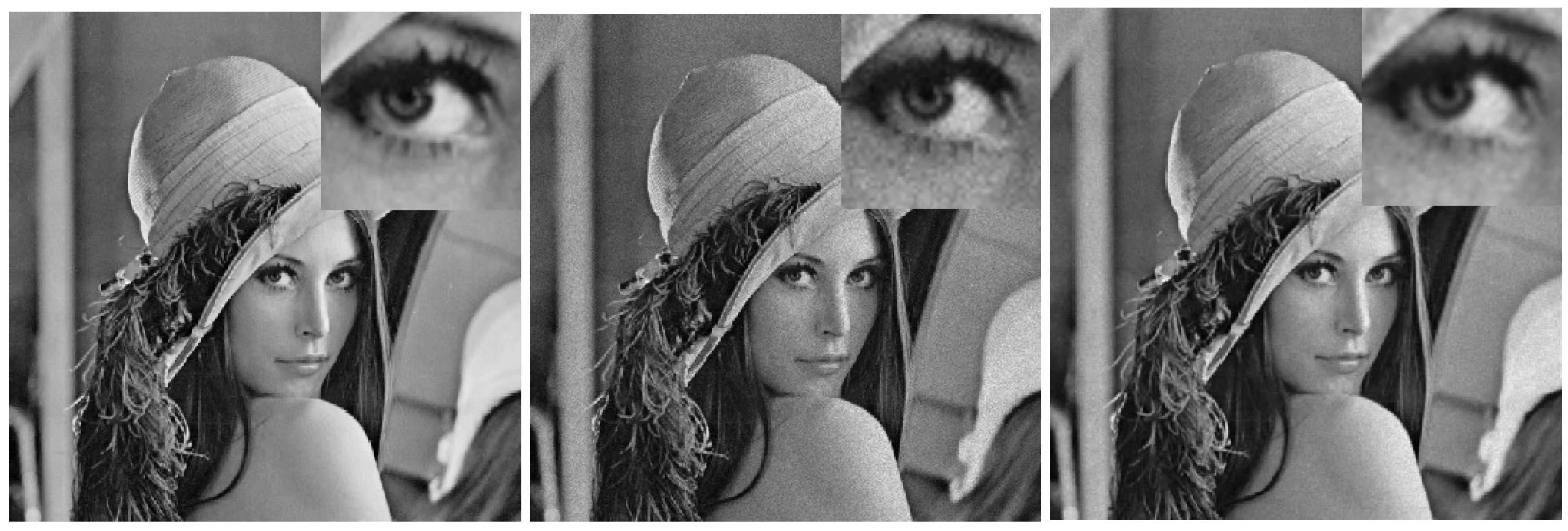
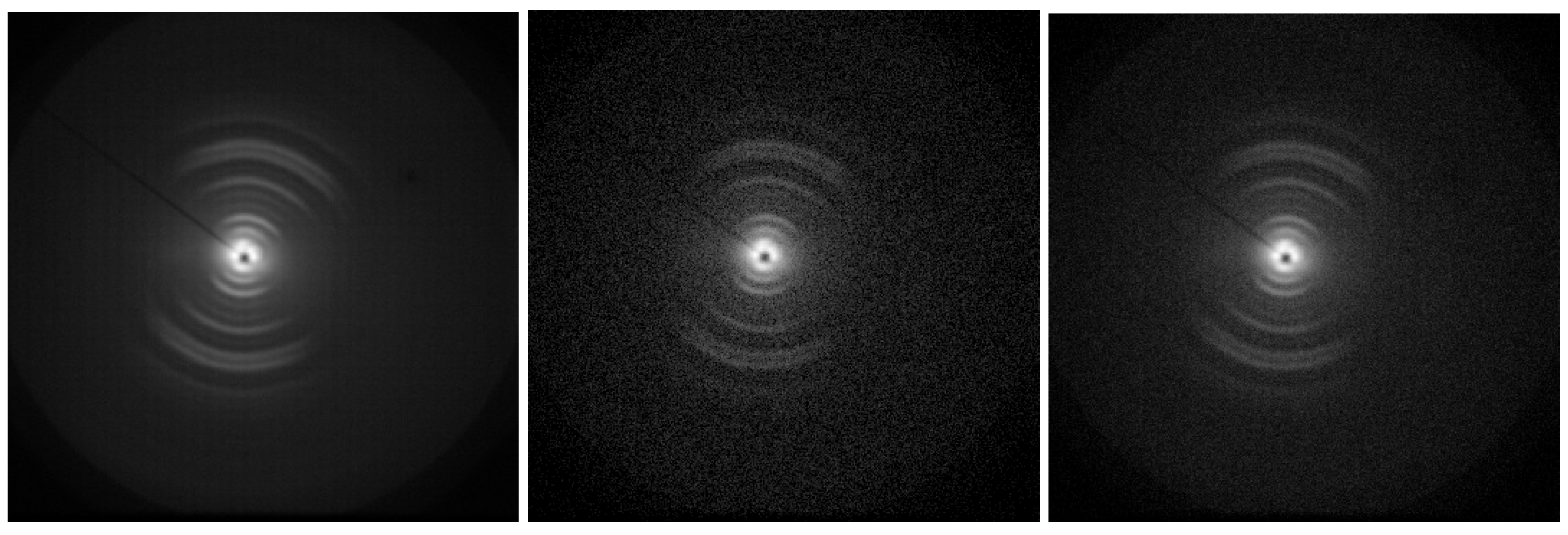
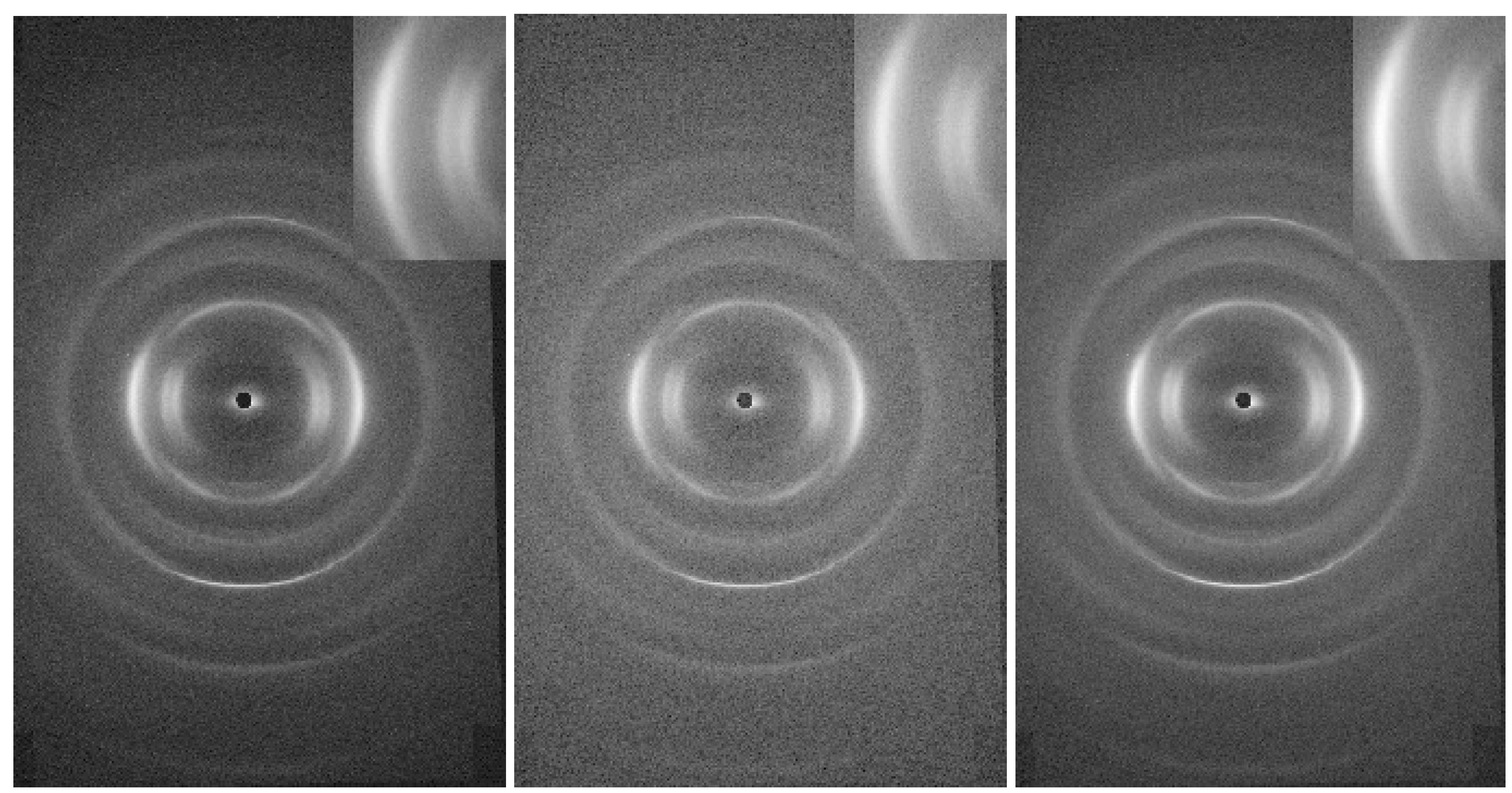
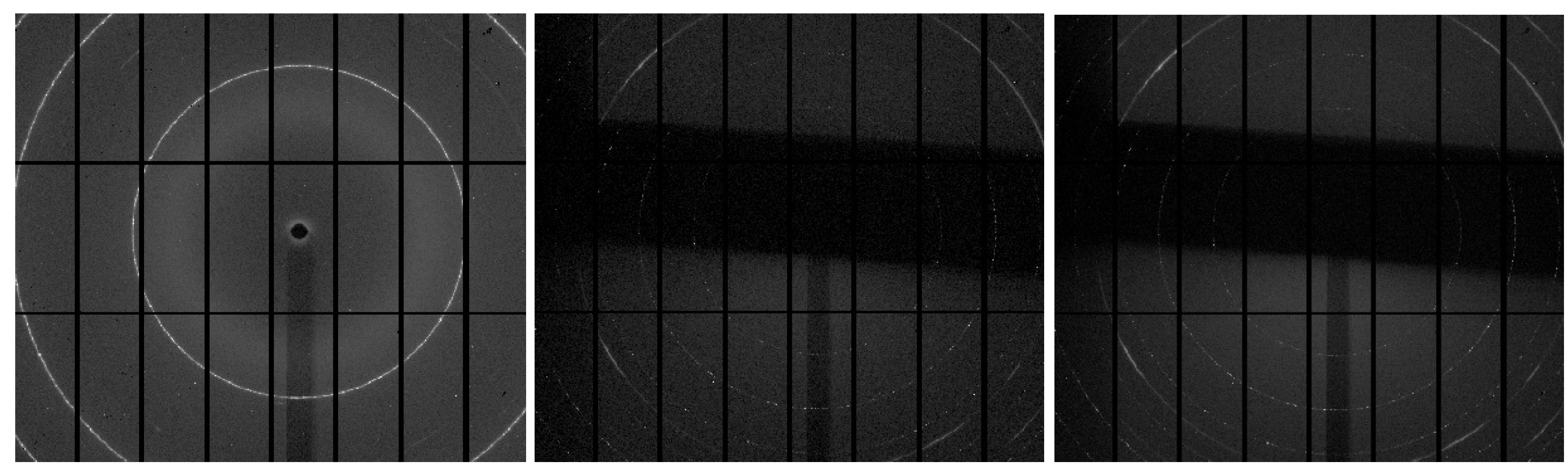
Figure 1. Noiseless image (left): original Lenna image with clear details and no visible distortion. Noisy image (centre): the same image affected by gaussian noise 5 % , compromising detail and clarity. Denoised outcome (right): improved image after applying the denoising algorithm. The close-up images on the upper right corner reveal restored details and reduced noise.
Preprints 142671 g001
Figure 2. Noiseless image (left): high statistics rat tendon image with clear details and a preferred orientation displayed by the π -symmetric partial arcs. Noisy image (centre): the same image affected by a poissonian noise due to a collection time of 2400s only. Denoised outcome (right): improved image after applying the denoising algorithm.
Preprints 142671 g002
Figure 3. Noiseless image (left): original high count rate sam4 XRD image with clear details. Noisy image (centre): the same image affected by a poissonian noise due to a low count statistics. Denoised outcome (right): improved image after applying the denoising algorithm. The close-up images on the upper right corner spot the reduced noise.
Preprints 142671 g003
Figure 4. Noiseless image (left): high statistics S043XX image collected at the PSI synchrotron radiation facility with clear details. Noisy image (centre): the same image affected both by a poissonian noise due to a short collection time and by a shadowing anomaly. Denoised outcome (right): improved image after applying the denoising scheme.
Preprints 142671 g004
Table 1. Improvement of the PSNR and SSIM values with the use of the denoising procedure in the cases of images with gaussian (Lenna) and poissonian (XRD) noise with the corresponding values of α and β .
image Lenna rat tendon sam4 S043XX
resolution 512×512 1024×1024 1600×2500 1679×1475
α 1.15 0.85 0.85 0.85
β 2.0 1.25 1.25 1.25
noise 0.05 - - -
PSNR (ini.) 31.33 25.94 30.91 18.10
PSNR (fin.) 34.76 30.76 34.75 18.28
SSIM (ini.) 0.59 0.10 0.60 0.12
SSIM (fin.) 0.64 0.27 0.67 0.14
Disclaimer/Publisher’s Note: The statements, opinions and data contained in all publications are solely those of the individual author(s) and contributor(s) and not of MDPI and/or the editor(s). MDPI and/or the editor(s) disclaim responsibility for any injury to people or property resulting from any ideas, methods, instructions or products referred to in the content.
Copyright: This open access article is published under a Creative Commons CC BY 4.0 license, which permit the free download, distribution, and reuse, provided that the author and preprint are cited in any reuse.
Prerpints.org logo

Preprints.org is a free preprint server supported by MDPI in Basel, Switzerland.

Subscribe

Disclaimer

Terms of Use

Privacy Policy

Privacy Settings

© 2026 MDPI (Basel, Switzerland) unless otherwise stated