Submitted:
09 December 2024
Posted:
10 December 2024
Read the latest preprint version here
Abstract
There is increasing observational evidence from the Hubble Space Telescope and the James Webb Space Telescope missions that we do not inhabit an expanding universe as described by the ΛCDM cosmological model, but rather a static universe. Such a universe has been postulated as the natural consequence of an extended theory of gravity that is based on the Exochronous (timeless) metric, ΣGR. The main challenge that faces any static universe model is the need to account for the observed cosmological redshift-distance relationship, as defined by the Hubble parameter. Up to now this has been explained by the so-called `tired light’ effect, but this suffers from numerous shortcomings. We propose here a mechanism based on the contraction of atomic matter: the Jeans Contraction, named after the physicist who first suggested this phenomenon as a source of cosmological redshift. We show how this postulated contraction of atomic matter is in fact a natural and inevitable consequence of the application of the Schwarzchild metric of General Relativity.
Keywords:
static universe
; redshift
; Schwarzchild metric
; tired light
1. Introduction
1.1. Historical Background
The currently prevailing cosmological paradigm - the CDM Hot Big Bang (plus inflation) model - with its image of an expanding universe, has over time become such an inescapable part of the cosmological landscape that we sometimes overlook the historical fact that this was not always the case. In 1917, only two years after formulating his General Theory of Relativity (GR), Einstein sought to apply his new theory to the dynamics of the universe as a whole in his ground-breaking paper: ‘Cosmological Considerations in the General Theory of Relativity’ [1]. The prevailing concept of the universe at that time was that it was static in nature and consisted largely of our own Milky Way galaxy surrounded by a somewhat sparse collection of nebulae. Not surprisingly then, Einstein sought to formulate a spacetime metric that conformed to this pre-conceived image - the so-called Einstein Static Universe (see [2] for a comprehensive review of Einstein’s paper). It was subsequently pointed out that the solutions to Einstein’s field equations of GR using his static metric, even with the inclusion of his cosmological constant, , were unstable to small perturbations and could not therefore be a viable representation of our universe. The next major development in applying GR to cosmology came from Friedman’s 1922 paper [3], in which the author examined the possibility of the curvature radius in the spacetime metric varying as a function of time. This became known as the Friedman-Lemaître-Robertson-Walker (FLRW) metric and gave rise to the well known Friedmann equations for the dynamical behaviour of the universe, which to this day form the cornerstone of the CDM cosmological model.
Observational evidence that our universe is in fact expanding in the manner predicted by Friedmann came with Hubble’s measurements of the redshifts of distant galaxies, where he found that the magnitude of the observed redshift was proportional to the galaxy’s distance from the observer [4]. The expanding universe model was not without its challengers, most notably the steady state model proposed by Hoyle [5], which described an expanding universe in which the average matter density remained constant over time due to the continuous creation of interstitial matter. Ultimately, the debate was resolved in favour of the Big Bang expanding universe with the 1966 discovery by Penzias and Wilson of the Cosmic Microwave Background (CMB) radiation, which confirmed that the universe had begun in an extremely hot, dense state and had subsequently cooled as it expanded. The final main building block of the CDM cosmological model was the 1998 discovery by the Supernova Cosmology Project [6] and the High-Z Supernova Search Team [7] of the acceleration in the cosmic expansion rate. This observed acceleration was best explained by a manifestation of Einstein’s original cosmological constant, , which can be thought of as a form of dark energy exerting a negative pressure that causes the expansion rate to accelerate.
Since that date, the CDM Big Bang paradigm has remained the prevailing cosmological model and the benchmark against which all astronomical observations are tested. Its continued success is based on the fact that the model can be described by a relatively small number () of free parameters and provides level fits to most astronomical observations; the only major drawback being the need to include the two hypothetical and, to date, unidentified components that give the model its name, i.e. dark energy (or ) and Cold Dark Matter (CDM). In spite of the success of the CDM model (see [8] for an overview), it is not without its issues. Arguably the most prominent of these issues is the so-called tension (see [9] for a detailed review), arising from the difference between local measurements of the Hubble parameter from a supernova and cepheid based distance ladder and calculated from CMB measurements.
1.2. Recent Observational Developments
The CDM model has proved to be a useful description of the evolution of our universe and in close accord with observational data in the redshift range . However, in recent years satellite based observatories such as the Hubble Space Telescope (HST) and the James Webb Space Telescope (JWST) have enabled astronomers to probe galaxies out to much higher redshifts; as far a in the case of JWST. This has made it possible to carry out detailed measurements on galaxies that came into existence close to the birth of the universe. The data from these high-z surveys have produced results that are hard to reconcile with the CDM cosmological model. Some of these findings are summarised in the following sections.
1.2.1. Galaxy Surface Brightness Evolution
The Tolman surface brightness (SB) test [10] was originally devised as a test for verifying the expansion of the universe, based on the variation in the SB of a galaxy as a function of redshift. In an expanding universe, SB should decrease as : one factor of (1+z) is due to time-dilation (decrease in photons per unit time), one factor is from the decrease in energy carried by photons, and the other factor of being due to the object having a larger apparent angular size. In [11] the authors analyse the UV SB of luminous disk galaxies from the HUDF and GALEX datasets, spanning from the local Universe to a redshift of . This analysis was subsequently extended in [12] to include elliptical galaxies at higher redshifts. Their findings suggest that the surface brightness remains constant, challenging the standard expanding universe cosmological model, and consistent with a static universe model.
1.2.2. The Distance Duality Relationship
The Etherington distance-duality relation (DDR) [13] describes the relationship between the luminosity distance of standard candles and the angular diameter distance in an expanding universe and is defined by the equation
where is the redshift, is the luminosity distance and the angular diameter distance. This relationship does not depend on specific cosmological models, so it can be used to test the expanding universe. The corresponding DDR for a non-expanding universe is
In [14] the author uses two independent samples of ultra-compact radio sources observed at 2.29 GHz and 5.0 GHz to test this relationship. They find that the observed radio luminosities systematically increase with redshift, and the DDR results are consistent with a non-expanding universe. This poses a challenge to the standard cosmological model, suggesting that either we live in a static universe, or that the size and luminosity density of ultra-compact radio sources evolve in a way that mimics a non-expanding universe.
1.2.3. Angular Diameter Distance
The relationship between angular diameter distance and redshift is a well defined signature of an expanding universe, with standard CDM cosmology predicting an inflection point in the curve at . (See Section 4.2.1 for a more detailed discussion on this topic). In [15] the authors analyse the angular diameters of a sample of high redshift galaxies obtained from the HST, and another sample of ultra high redshift galaxies obtained from the JWST and compiled from the results gathered by a number of research teams. They conclude that the measured angular diameters are not consistent with the predictions from the CDM model but are a good fit with the predictions from a static universe cosmology, such as the tired-light model. The only way of reconciling the observed angular diameters with CDM predictions would be to postulate that average galaxy sizes evolve with decreasing redshift.
1.2.4. Superabundance of Large Galaxies at High Redshifts
Galaxy formation models generally assume that large galaxies, such as those observed today at low redshifts, are formed by the merger of smaller galaxies over time. Such models will therefore predict that any galaxies observed early in the life of the universe are likely to be relatively small in comparison to the later generation of galaxies observed at low redshifts. However, results from the analysis of 88 galaxies in the redshift range using the NIRcam instrument on the JWST, as reported in [16], reveal a much higher number of large galaxies at these high redshifts than predicted based on the age of the universe as calculated from the CDM model.
Similarly, a study published in [17] describes the discovery of 6 massive galaxies with stellar masses greater than at redshifts in the range and finds that the stellar mass density in massive galaxies during this period is much higher than previously anticipated, challenging existing models of galaxy formation and evolution.
Another study examining the structure, composition and formation of massive red galaxies at redshifts greater than 6 using photometric data from the JWST [18] finds that the apparent age of these galaxies ranges from 0.9 to 2.4 Gyr, which is in conflict with the calculated age of the universe at these redshifts based on CDM cosmology. The authors conclude that their findings would be better explained by a cosmological model in which there is a much expanded timeline in which galaxies can evolve at any given redshift, such as the model proposed in [19].
In [20] the authors analyse the photometric and kinematic properties of a number of galaxies captured by the JWST with redshifts of . The photometric data suggestd that these galaxies are too large and too bright to have formed within the short timescale of Gyr implied by the CDM model. Similarly, the observed galaxy morphology reveals a prevalence of spiral galaxies that mimic the characteristics of more recent galaxies observed at low redshifts, which cannot readily be explained by existing galaxy formation models. The authors suggest that the answer may lie in alternative cosmological models that could potentially explain the rapid clustering of baryonic matter into stars and galaxies, and they propose Modified Newtonian Dynamics (MOND) [21] as a possible model.
Even before the launch of the JWST satellite, ground based surveys were identifying large scale structures at high redshifts that were too massive to have formed by the time-frame implied by their measured redshifts using the CDM model. In their article titled "The impossible early galaxy problem" the authors of [22] report on the abundance of high mass halos, with at redshifts in the range .
1.2.5. Ionization History
We know that following the epoch of recombination, the resulting neutral hydrogen in the universe was progressively reionized by UV radiation emitted by early stars. Analysis of CMB data by the Planck satellite mission indicates that this process took place at redshifts in the range . However, analysis of the galaxies observed by JWST, as reported in [23], concludes that they produce more ionizing photons than previously thought, which could lead to reionization occurring too early at around . This excess of photons in the early universe has been termed the "photon budget crisis".
1.2.6. Supermassive Black Holes
The growth rate of supermassive black holes such as those found at the centre of galaxies is constrained by the Eddington-limited accretion rate. The recent discovery by the JWST of a X-ray luminous supermassive black hole, UHZ-1, with a mass of at a confirmed spectroscopic redshift of is therefore difficult to explain within the framework of the CDM model. This object should have taken over 700 Myr to grow via standard Eddington-limited accretion whereas its measured redshift corresponds to an age of only Myr after the birth of the universe. The author of [24] suggests that this is indicative of an overly compressed cosmological timeline implied by the CDM model, and suggests as an alternative the model, which has a much more gradual evolution rate as a function of redshift, and is functionally equivalent to the Milne empty universe model [25].
1.3. Alternative Cosmological Models
The common feature of all the observational anomalies described above in Section 1.2 above is that they describe phenomena that are better explained by a non-expanding universe or a universe in which the evolution of the cosmic scale factor does not follow the predictions arising from the application of the CDM model and hence the relationship between cosmic age and redshift is untenable. Several alternative cosmological models have been postulated by a number of authors that have the potential to account for one or more of these observational anomalies. We briefly review two such models here.
1.3.1. Modification Of Newtonian Dynamics (MOND)
MOND was first proposed by Milgrom [26] as an alternative to dark matter in explaining how large scale structure could form in an expanding universe. Subsequently in 1998 (i.e. prior to the JWST mission) Sanders showed that MOND could successfully account for the early () formation of massive elliptical galaxies as a result of monolithic dissipation-less collapse. In [20] it is suggested that this could account for the abundance of large and apparently mature galaxies at high redshifts observed by JWST.
1.3.2. Static Universe Models
Although Einstein’s original static universe was ultimately shown to be unstable [2], there have been more recent attempts to construct a viable static universe model. One such model is the Exochronous Universe described in [27], which is associated with a novel static solution to the Einstein field equations of General Relativity, in which the usual time dimension of GR is replaced by a hyperspatial foliation dimension. This model describes a static, i.e. non-expanding, universe in which successive metric foliations give rise to an accumulating gravitational potential that mimics the effects of dark matter.
1.4. Accounting for Redshift in a Static Universe
Although a static universe can account for many of the high redshift observational anomalies described in Section 1.2, it has the apparently serious drawback that it is at first sight incompatible with the observed Hubble distance-redshift relationship. (It is interesting to note that even Hubble was not convinced that cosmological redshifts were due to the expansion of the universe [28], and felt that other factors could be causing his redshift observations.) This leads to the question that forms the core of this article: how can a static universe give rise to a time-varying cosmological redshift?
1.4.1. Tired Light
Several authors cited in Section 1.2 have referenced a `tired light’ mechanism as a synonym for the static universe [15,29]. The concept of tired light was originally introduced by Zwicky [30]. In this work, Zwicky analysed three possible physical mechanisms that could provide the necessary energy loss of photons on their path through spacetime:
- Compton scattering on free electrons
- Gravitational redshift due to gravitational potential wells of galaxies or galaxy clusters along the photon’s path
- General-relativistic transfer of photon energy/mass to the masses distributed along the photon’s path
Interestingly, Zwicky did not include Thomson scattering or double-Compton scattering in his analysis, both of which are known to occur in the early universe. The main problem with tired light models is that, whilst they may account for the observed redshift, they do not result in the creation of inter-particle space that is an essential characteristic of the expanding universe model. Without this phenomenon, the universe would still be in a high density state today. We review some of these tired light mechanisms in greater detail in Section 2.
1.4.2. The Jeans Contraction
An alternative redshift mechanism that does not suffer the drawbacks associated with the tired light model is one that was first proposed by the British astronomer, Sir James Jeans [31], perhaps best known for giving his name to the Jeans length, which determines the conditions for galaxy formation from a gas cloud. To quote directly from the article in which he made this proposal: "Another possibility - nearly but not quite identical with the foregoing - is that the universe retains its size, while we and all material bodies shrink uniformly. The red shift we observe in the spectra of the nebulae is then due to the fact that the atoms which emitted the light millions of years ago were larger then than the present-day atoms with which we measure the light - the shift is, of course, proportional to distance. The final end here is a universe in which all matter has shrunk to nothing."
In the remainder of this paper we refer to this mechanism as the "Jeans Contraction", and it is discussed in more detail in Section 3.
1.5. Outline
Following this introductory section, this paper is organised as follows. Section 2 examines the role that a tired light model can play in accounting for redshift. Section 3 describes a mechanism for generating the Jeans Contraction, in which a particle’s size is dynamically determined by its self-gravitational potential and the background gravitational potential of the universe as a whole in the Exochronous metric associated with the GR paradigm. In Section 4, we calculate how the scale factor evolves over time under the Jeans Contraction mechanism, and show how the resulting redshift-distance and redshift-time relationships can provide a natural explanation for the observational anomalies identified in Section 1.2 above. Finally, Section 5 summarises the main consequences arising from this novel interpretation of redshift.
2. Tired Light Models
In this section we review in greater depth some of the tired light mechanisms identified in Section 1.4, and we also examine the Double Compton scattering process as a potential source of redshift.
2.1. Gravitational Well Redshift
Probably the best known example of photon energy loss (or gain) on cosmological scales due to gravitational effects is the Integrated Sachs-Wolfe (ISW) effect, in which photons transiting a cosmological void will become redshifted (i.e. lose energy) as they enter the void but will not regain all that energy as they exit the void due to the expansion of the universe in the intervening time, resulting in a net loss of photon energy and an overall increase in redshift. While the ISW effect is readily observable in CMB maps, it is difficult to devise a model in which the ISW mechanism could result in a cumulative increase in observed redshift with increasing distance from an observer, since any redshift gains resulting from transiting voids will on average be cancelled out by corresponding blueshifts from transiting galaxy clusters. Gravitational well redshift is therefore unlikely to be a good candidate for the origin of the Hubble redshift-distance relation.
2.2. Thomson Scattering
Thomson scattering is the elastic scattering of photons by free electrons
The effect can be observed in the polarisation of the CMB. However, because it is an elastic collision, there is no overall photon energy loss and this effect cannot therefore be a plausible tired light mechanism.
2.3. Double Compton Scattering
Double-photon Compton (DC) scattering is a third order process in which an incident photon interacts with an atomic electron and the collision products are one recoil electron and two emitted photons, each of lower energy than the incident photon.
The DC scattering effect plays an important role in maintaining thermal equilibrium in the photon-electron plasma that exists in the early universe prior to recombination [32]. In a conventional CDM expanding universe it is generally assumed that the energy of the CMB photons will fall as they are redshifted, such that
and consequently these low energy photons will no longer interact with the neutral hydrogen atoms that predominate in the post-recombination epoch. However, in a static (non-expanding) universe, CMB photons do not undergo any energy loss and retain the energies that they had at the time of recombination. These energetic CMB photons therefore become increasingly out of thermal equilibrium with the baryonic matter content of the universe. However, this situation only persists up to the epoch of reionization at , at which point the energetic CMB photons are again able to interact with ionized hydrogen via the DC process. From this reionization redshift up to the present day, the DC mechanism is responsible for keeping the CMB photons in thermal equilibrium with baryonic matter, via the creation of additional lower energy photons. Figure 1 shows how the baryon/photon ratio, , evolves as a function of redshift.
2.4. Primordial Nucleosynthesis
Although it is to some extent outside the scope of this article, it is perhaps worthwhile describing a hypothetical, but still plausible, scenario that would give rise to the starting conditions in Figure 1, i.e. a primordial baryon/photon ratio of at a redshift of and a temperature of K. In the standard Hot Big Bang model reheating following inflation raises the temperature of the universe to GeV, after which it cools as the universe expands. Particle species condense out of the primordial plasma as their rest mass energies fall below the plasma energy. At the appropriate temperature protons and anti-protons are assumed to be generated, but with a so-far unexplained asymmetry in their numbers of the order of one part in , resulting in a small excess of what we would term baryonic matter. The remaining protons and anti-protons annihilate generating a corresponding number of photons that persist to the present day in the form of the CMB. The assumption in standard CDM cosmology is that the number of photons in the CMB remains constant from that point onwards, so that the baryon/photon ratio observed today remains unchanged from its value in the early universe.
An alternative scenario that we describe here is based on the idea that the universe originates from a primeval atom (q.v. Lemaître [33]) that evolves into a primordial neutron cloud. Photons are then created, firstly by the -decay of primordial neutrons, and subsequently by the fusion of protons and neutrons to form deuterium and ultimately helium, with the release of energetic photons corresponding to the binding energy of deuterium. This chain of reactions results in a primordial baryon/photon ratio of at a redshift of and a temperature of K. Another feature inherent in a static universe model is that, since CMB photon energy is constant and no longer a function of redshift, there will be no epoch of radiation-matter equality such as exists in CDM cosmology. In general, ignoring the relatively small amount of energy conversion from baryonic rest mass to radiation resulting from nuclear fusion in stars, the ratio will remain essentially constant throughout the evolution history of the universe. We can verify the validity of this assumption by first calculating the radiation energy per baryon created during the epoch of primordial nucleosynthesis via the reactions
The photon energies released in reactions [1], [2] and [3] are , and respectively. Assuming that the proportion of nucleons at the end of the epoch of primordial nucleosynthesis is broadly the same as that observed in the present day universe, i.e by mass is hydrogen, and is helium, then the proportion of primordial neutrons that must have beta decayed to protons via reaction [1] is . The remaining of the primordial neutrons then go on to form deuterium, 3He, and ultimately 4He, via reactions [2],[3], [4] and [5]. The precise amount of energy liberated in the form of photons as opposed to increasing particle kinetic energy will depend on the relative reaction rates of [3] and [4], the calculation of which is beyond the scope of this article. Assuming that approximately of deuterium is processed via reaction [3] then we obtain the following photon energy output per primordial neutron:
This gives a primordial photon/baryon energy ratio of
We can compare this with the present day values of and . From Planck CMB measurements [34] we obtain an energy density of , which yields about . The same source provides us with a value for the baryonic mass fraction of the universe of , where . This equates to a baryonic matter density of and hence a baryonic energy density of . The resulting present day photon-baryon energy ratio is therefore , which is very close to the hypothetical ratio at the time of primordial nucleosynthesis given in Equation 5. The fact that these estimates are of the same order of magnitude gives some credibility to the conjecture that a tired light mechanism based on the DC scattering process could indeed be a plausible source of redshift in a non-expanding universe.
3. The Jeans Contraction
3.1. Possible Candidates for Matter Contraction
In his imaginative suggestion that the Hubble redshift could be due to the contraction of atomic matter, Jeans did not speculate on the actual mechanism that might give rise to this contraction. In this section we will seek to develop a plausible model that, ideally, would be based on existing, well established, physics.
Although Jeans’ proposal might at first appear outrageous, we should not be too concerned about the concept of atoms shrinking. After all, we are familiar with this from both Special and General Relativity. In Special Relativity, the phenomenon of Lorentz contraction for an object in motion relative to an observer is well established:
where L is the length measured by an observer in motion relative to the object, is the proper length of the object in its rest frame, and is the Lorentz factor, given by
We also have the related phenomenon of relativistic time dilation:
where is the observed time interval and is the rest frame time interval. However, the Lorentz contraction is unlikely to be of much relevance as a potential mechanism for atomic particle contraction since, in general, we are dealing with particles at rest rather than in motion.
In General Relativity, we are familiar with the concept of gravitational time dilation. From the Schwarzchild metric of GR:
we can write down the expression for gravitational time dilation:
where is the Schwarzchild radius of a gravitating mass M, defined as
is the time for an observer at a distance of r from the mass, and is the time experienced in the absence of gravity. We note from eqn:Equation 10 that , i.e. time slows down in regions of stronger gravitational potential. This phenomenon is well proven experimentally to the extent that modern day measurements are able to detect the gravitational time dilation arising from changes in a clock’s altitude of as little as 1 m in the Earth’s gravitational field [35]. The phenomenon of gravitational time dilation has little practical application in everyday life, other than the need to take it into account in accurately measuring the time recorded by atomic clocks used in satellite navigation systems such as GPS.
We are perhaps less familiar with the phenomenon of gravitational length contraction, although this also follows directly from the Schwarzchild metric of Equation 9, giving:
This can best be illustrated by the diagram in Figure 2, where we can see that the distance element in flat Euclidean space, is less than the distance in the Schwarzchild metric, .
We also note that the length contraction in the Schwartzchild metric, , is equal and opposite to the time dilation, , which of course is necessary in order to maintain Lorentz invariance. This tells us that the dimensions of the atoms in an atomic clock must change in the presence of a gravitational potential so as to give rise to the observed gravitational time dilation effect.
An example of where this phenomenon is utilised in scientific experiments is that of gravitational wave detectors based on laser interferometry. These make use of the fact that the spacing of mirrors used to reflect the laser beams in the interferometer is modulated due to the passage of a gravitational wave through the detector. The effect is extremely small, but nevertheless measurable. For example, the LIGO gravitational wave observatory is able to detect changes of as small as m in the length of its 4km long arms.
3.2. Quantifying the GR Length Contraction Effect
Having established the fact that atomic dimensions do indeed contract in the presence of a gravitational potential gradient, we now need to ask ourselves whether this phenomenon is in itself sufficient to give rise to the Jeans Contraction, i.e. the progressive contraction in atomic size over time. In effect, we are seeking to ascertain whether a proton’s self-gravity is sufficient to cause it to contract. We can readily calculate the magnitude of the contraction by determining the proton’s Schwarzchild radius, which, using standard value for the proton mass in Equation 11, gives m. We are interested here in determining the contraction of a hydrogen atom rather than the proton itself, as it is this parameter that will determine the frequency of photons emitted by stars that we can actually measure. Using the reduced Compton wavelength of an electron m as the most appropriate value for r, we find that . This is clearly a minuscule effect, but we should bear in mind that this value is the one-off instantaneous effect of subjecting a proton to its own gravitational field. If we consider the proton as being essentially an oscillating field then the gravitational contraction calculated above is the contraction experienced per oscillatory cycle. To calculate the contraction rate per second we need to exponentiate the per-cycle change in scale factor from Equation 12 by the proton Compton frequency, thus:
In practice, the calculation of is simplified by performing a Binomial expansion of the right hand side of Equation 13
where and . Since x is very small, we can effectively ignore all terms in and higher order, giving us this simplified expression for the scale factor evolution rate
Taking the proton Compton frequency, given by , this gives a value of for the contraction frequency (). Is this a reasonable value?
At this point it is perhaps worth pausing to consider how the Hubble parameter is determined in standard CDM cosmology. This model does not define any physical process that gives rise to the expansion of the universe. The growing scale factor is merely a mathematical artefact of the Friedman equations. Hence it is not possible to directly calculate a value for the Hubble parameter at some point in the evolution history of the universe. Rather, it is necessary to determine the present day value of the Hubble parameter, , by directly measuring the redshift-distance relationships of objects in the local universe. Then armed with this value of one can calculate the value of at any earlier redshift using the evolution equation derived from the Friedman equations (see Equation 25). In contrast, if the Jeans Contraction is the correct description of the redshift mechanism in our universe then it should in principle be possible to determine the rate of such contraction from a calculation that involves only quantities that can be measured locally. The only obvious quantities that can reasonably be involved in such a calculation are the Newtonian gravitational constant, G, the speed of light c, the Planck constant h, and the proton mass . It is these same quantities that we have used in Equation 11 and Equation 15 to calculate the present day value for .
Returning to our calculated value of for the contraction rate, we can compare this to the present day measured value of the Hubble parameter, . So whilst we note that our calculated value for is approximately double the currently measured value, and as such represents arguably the worst evaluation of the Hubble parameter since Edwin Hubble’s own efforts (H = 500 km/s/Mpc in 1929 [4]), it is nevertheless evident that a simple application of the principle of gravitational length contraction to a system consisting of a hydrogen atom evolving in its own gravitational field leads to a derivation of that is of the same order of magnitude as the value obtained from local distance ladder measurements.
3.3. Evolution of Length Contraction
Returning to Equation 12, we note that is itself a function of r, such that the contraction factor increases as the particle radius decreases, leading to a continued contraction. It is therefore of interest to observe how this contraction evolves over time, by solving for in this differential equation, thus:
However, the resulting solution is somewhat unwieldy, so it is more informative to make use of the relationship
where w is the curvature dimension in the Schwarzchild metric. Substituting for in Equation 12 we obtain
Solving this differential equation gives us
and in fact it is this parabola of Equation 19 that is plotted in Figure 2 as a visual representation of the Schwarzchild metric. The evolution of the particle contraction is illustrated in the animation in Figure 3.
4. Evaluation
4.1. Evolution of Hubble Parameter with Redshift
In Section 3 we have seen that the Jeans Contraction, resulting from atomic matter contraction in the Schwarzchild metric of GR, can account for the observed present day value of the Hubble parameter . We now wish to ascertain how this parameter varies as a function of cosmological redshift, and how this impacts on the calculated age of the universe at different redshifts.
At first sight, based on Equation 15, we might expect the calculated value of the conformal Hubble parameter to remain constant as a function of redshift, since there is no change to the quantities involved in the atomic reference frame. Hence we would expect to see a constant value for over the entire redshift history; an identical result to the expansion history applicable to the so-called Milne universe in standard CDM cosmology, in which and . This is illustrated in the left hand plot of Figure 4. The right hand plot shows the standard proper-time Hubble parameter .
However, there is one important factor that we have overlooked in determining the evolution of : we have assumed that in Equation 15 remains constant. This assumption is not valid if we are examining the implications of the Jeans Contraction in an otherwise static universe as described in [27]. The GR model defined there leads to a time-varying Newtonian gravitational "constant", G, such that
where is the present-day measured value of the Newtonian gravitational constant, defines the fundamental gravitational scaling factor
where R is the Hubble radius of the universe, and is the total baryonic mass contained within the Hubble radius, and is the metric foliation factor, defined as
where and are respectively the foliation indices at the present day and at the end of the era of baryogenesis. (See section 4 of [27] for a detailed derivation).
So we now need to incorporate the implications of a varying G into Equation 11, giving
and Equation 15 becomes
The effects of incorporating the evolving gravitational scaling factor into the Jeans Contraction are illustrated in Figure 4.
4.2. Fit With Observational Data
In this section we examine the impact of the evolution of the Hubble parameter under the Jeans universe on a number of cosmological distance and time measures, as a function of redshift.
4.2.1. Angular Diameter Distance
We are interested in the relationship between angular diameter distance and redshift as this determines the apparent size of distant galaxies. The angular diameter distance is defined as the ratio of an object’s physical transverse size to its angular size (in radians) and is defined as
where is the comoving distance, which itself is defined as
with the Hubble evolution function being defined as
Combining Equation 23 and Equation 24 we obtain an expression for angular diameter distance:
The corresponding equation for non-expanding universe based on the Jeans model is:
with and hence for the Jeans and tired-light models.
These quantities are plotted in Figure 5 for various cosmological models, including CDM and Jeans. From this it is evident that the tired-light (or Milne) and Jeans universes lead to angular diameter distances that increase monotonically with redshift over the entire evolutionary history, and do not exhibit the inflection point at that is a feature of CDM cosmology.
The angular diameter distance and angular size of an object are inversely related related thus
This relationship is plotted in Figure 6, which shows how the angular diameter of an object of fixed size (about the size of a typical galaxy) increases with redshift for different cosmological models. From this we can see that the static universe models do not exhibit the inflection point that is a feature of the CDM universe. We can now compare this figure with the corresponding Figure 5 in [15], from which we can conclude that the angular diameter of distant objects in a Jeans universe results in a much better fit with JWST observational data than does the standard CDM cosmology.
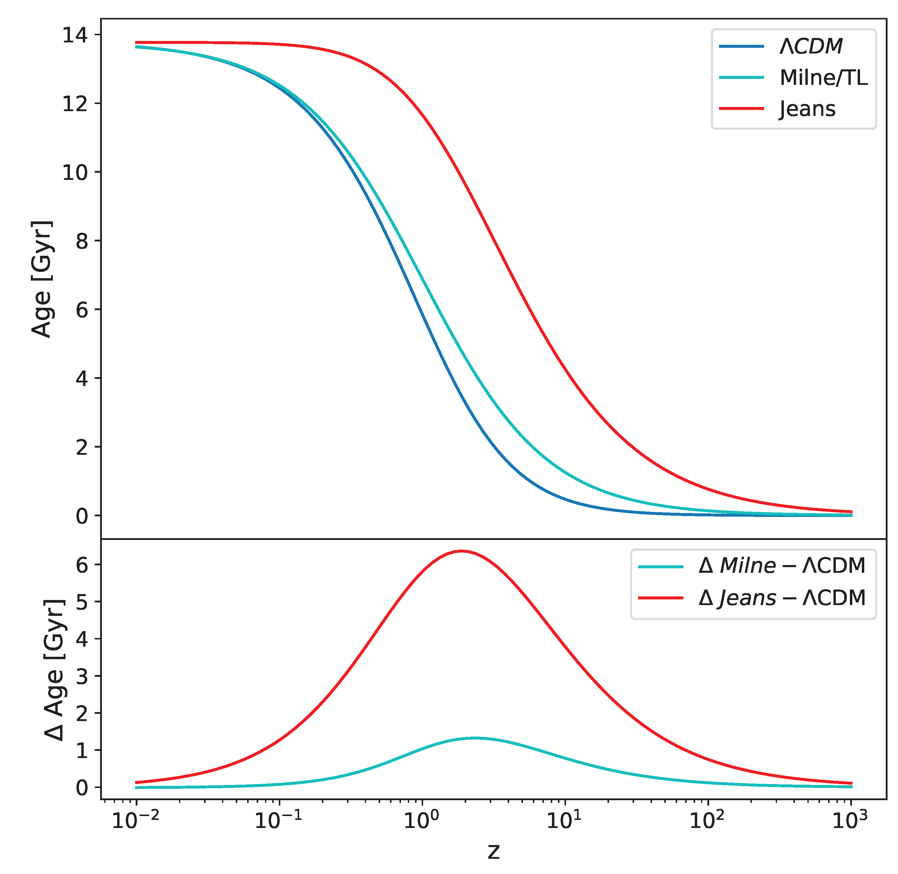
4.2.2. Age of Universe
The age of the universe as a function of redshift is an important quantity as it determines how long various processes such as star and galaxy formation, reionization, and the creation of various heavier elements have had to operate at a given redshift. The cosmological age T is defined as
and for the Jeans universe
This quantity is plotted in the upper part of Figure 7 for various cosmological models. The bottom part of this figure shows the age difference between each cosmological model and the base-line CDM cosmology. From this it is evident that both tired-light and Jeans models result in a substantially greater age at any given redshift than does the standard CDM cosmology. This difference is particularly marked in the case of the Jeans model, which has a maximum excess age of Gyr at a redshift of . Even at a redshift of , which corresponds to the redshifts of some of the most distant galaxies discovered by the JWST, we can see that these objects have had an additional Gyr in which to form as compared to the Myr that would be the case for the CDM model.
This increase in elapsed time for redshifts in the range is thus able to account for all the anomalous observational results identified in Section 1.2, including:
5. Conclusions
In this paper we have identified two possible mechanisms for generating redshift in a static universe. Firstly, a tired-light mechanism based on the well established double Compton scattering process, which we have shown can readily be applied to the generation of additional red-shifted photons in the CMB as the universe cools. We have demonstrated that this mechanism maintains to the present day the overall photon-baryon energy ratio that existed during the epoch of primordial nucleosynthesis, whilst massively increasing the baryon/photon ratio from its initial , to its observed present day value of . This process obviates the need to account for the matter-antimatter asymmetry in the early universe that would otherwise be required to explain this high value for . Whilst this Compton scattering mechanism provides a viable means for red-shifting CMB photons, it would on its own be insufficient to account for the increase in the interstitial space between matter particles that we observe as the universe evolves. This requires another entirely different mechanism.
Based on a concept originally suggested by Jeans [31], we have identified a process of atomic matter contraction that is entirely derived from the application of the Schwarzchild metric of standard General Relativity. This metric has been exhaustively tested on solar system scales [38] and has proved that GR provides a very precise agreement with observational results, such as light deflection by the Sun’s gravitational field, and the perihelion precession of Mercury. We have shown that, assuming that the domain of GR extends down to atomic scales, then this will inevitably lead to the phenomenon described by Jeans: that atomic matter, such as a hydrogen atom for example, will progressively contract in its own self-gravitational field. Thus our fundamental clocks and rulers will shrink, and light emitted by atoms in the past will appear red-shifted relative to a present day observer. The process will at the same time increase the apparent space between atoms, even though the average matter density will remain constant in the non-expanding universe. Furthermore, we have shown that the calculated rate of matter contraction arising from this effect lies very close to the currently observed value for the Hubble parameter, lending credence to the assertion that the Jeans Contraction is the true source of redshift in a static universe, as opposed to redshift being the consequence of an expanding universe based on the CDM Big Bang paradigm.
We have shown that the redshift-distance relation associated with the static universe provides a much better fit with observations of galaxy sizes and luminosities. We have also demonstrated that the redshift-age relationship resulting from the application of the Jeans mechanism results in much extended timescales between the birth of the universe and the epoch of star and galaxy formation, which explains the otherwise anomalous observations of galaxy counts, galaxy size and morphology, that are difficult to explain using the evolution timescales inherent in CDM cosmology.
In summary, the two redshift mechanisms identified in this paper give rise to a universe with an evolutionary history that more closely matches recent observations than a universe based on standard CDM cosmology, and they are consistent with a static universe model.
Funding
This research received no external funding.
Data Availability Statement
All the data analysed in this article are available from the references cited in the article.
References
- Einstein, A. Cosmological considerations in the general theory of relativity. Sitz. König. Preuss. Akad. 1917, pp. 142–152.
- O’Raifeartaigh, C.; O’Keeffe, M.; Nahm, W.; Mitton, S. Einstein’s 1917 static model of the universe: a centennial review. European Physical Journal H 2017, 42, 431–474. [Google Scholar] [CrossRef]
- Friedman, A. On the Curvature of Space. Gen. Rel. Grav. 1999, 31, 1991–2000. [Google Scholar] [CrossRef]
- Hubble, E. A relation between distance and radial velocity among extra-galactic nebulae. Proceedings of the National Academy of Sciences 1929, 15, 168–173. [Google Scholar] [CrossRef] [PubMed]
- Hoyle, F. On the Origin of the Microwave Background. ApJ 1975, 196, 661–670. [Google Scholar] [CrossRef]
- Perlmutter, S.; Aldering, G.; Goldhaber, G.; Knop, R.A.; Nugent, P.; Castro, P.G.; Deustua, S.; Fabbro, S.; Goobar, A.; Groom, D.E.; et al. Measurements of Ω and Λ from 42 High-Redshift Supernovae. The Astrophysical Journal 1999, 517, 565–586. [Google Scholar] [CrossRef]
- Riess, A.G.; Filippenko, A.V.; Challis, P.; Clocchiatti, A.; Diercks, A.; Garnavich, P.M.; Gilliland, R.L.; Hogan, C.J.; Jha, S.; Kirshner, R.P.; et al. Observational Evidence from Supernovae for an Accelerating Universe and a Cosmological Constant. The Astronomical Journal 1998, 116, 1009–1038. [Google Scholar] [CrossRef]
- Peebles, P.J.E. Status of the LambdaCDM theory: supporting evidence and anomalies. Philosophical Transactions A 2024. [Google Scholar]
- Di Valentino, E.; Mena, O.; Pan, S.; Visinelli, L.; Yang, W.; Melchiorri, A.; Mota, D.F.; Riess, A.G.; Silk, J. In the realm of the Hubble tension - A review of solutions. Classical and Quantum Gravity 2021, 38. [Google Scholar] [CrossRef]
- Tolman, R.C. On the estimation of distances in a curved universe with a non-static line element. Proc, Natl. Acad. Sci. 1930, 16, 511–520. [Google Scholar] [CrossRef]
- Lerner, E.J.; Falomo, R.; Scarpa, R. UV surface brightness of galaxies from the local Universe to z 5. International Journal of Modern Physics D 2014, 23. [Google Scholar] [CrossRef]
- Lerner, E.J. Observations contradict galaxy size and surface brightness predictions that are based on the expanding universe hypothesis. Monthly Notices of the Royal Astronomical Society 2018, 477, 3185–3196. [Google Scholar] [CrossRef]
- Etherington, I. On the definition of distance in general relativity. The London, Edinburgh, and Dublin Philosophical Magazine and Journal of Science. 1933, 15. [Google Scholar] [CrossRef]
- Li, P. Distance Duality Test: The Evolution of Radio Sources Mimics a Nonexpanding Universe. The Astrophysical Journal Letters 2023, 950, L14. [Google Scholar] [CrossRef]
- Lovyagin, N.; Raikov, A.; Yershov, V.; Lovyagin, Y. Cosmological Model Tests with JWST. Galaxies 2022, 10. [Google Scholar] [CrossRef]
- Finkelstein, S.L.; Leung, G.C.K.; Bagley, M.B.; Dickinson, M.; Ferguson, H.C.; Papovich, C.; Akins, H.B.; Arrabal Haro, P.; Davé, R.; Dekel, A.; et al. The Complete CEERS Early Universe Galaxy Sample: A Surprisingly Slow Evolution of the Space Density of Bright Galaxies at z = 8.5–14.5. The Astrophysical Journal Letters 2024, 969, L2. [Google Scholar] [CrossRef]
- Labbé, I.; van Dokkum, P.; Nelson, E.; Bezanson, R.; Suess, K.A.; Leja, J.; Brammer, G.; Whitaker, K.; Mathews, E.; Stefanon, M.; et al. A population of red candidate massive galaxies 600 Myr after the Big Bang. Nature 2023, 616, 266–269. [Google Scholar] [CrossRef]
- Lopez-Corredoira, M.; Melia, F.; Wei, J.J.; Gao, C.Y. Age of massive galaxies at redshift 8. arXiv preprint 2405.12665 2024. [Google Scholar] [CrossRef]
- Melia, F.; Shevchuk, A.S. The R h=ct universe. Monthly Notices of the Royal Astronomical Society 2012, 419, 2579–2586. [Google Scholar] [CrossRef]
- McGaugh, S.S.; Schombert, J.M.; Lelli, F.; Franck, J. Accelerated Structure Formation: The Early Emergence of Massive Galaxies and Clusters of Galaxies. The Astrophysical Journal 2024, 976, 13. [Google Scholar] [CrossRef]
- Sanders, R.H. Forming galaxies with MOND. Monthly Notices of the Royal Astronomical Society 2008, 386, 1588–1596. [Google Scholar] [CrossRef]
- Steinhardt, C.L.; Capak, P.; Masters, D.; Speagle, J.S. The impossible early galaxy problem. The Astrophysical Journal 2016, 824, 21. [Google Scholar] [CrossRef]
- Muñoz, J.B.; Mirocha, J.; Chisholm, J.; Furlanetto, S.R.; Mason, C. Reionization after JWST: a photon budget crisis? MNRAS 2024, 535, L37–L43. [Google Scholar] [CrossRef]
- Melia, F. The cosmic timeline implied by the highest redshift quasars. arXiv preprint 2412.02706 2024. [Google Scholar] [CrossRef]
- Milne, E. World-Structure and the Expansion of the Universe. Zeitschrift für Astrophysik 1933, 6, 1. [Google Scholar] [CrossRef]
- Milgrom, M. A modification of the Newtonian dynamics as a possible alternative to the hidden mass hypothesis. The Astrophysical Journal 1983, 270, 365–370. [Google Scholar] [CrossRef]
- Booth, R. The Exochronous Universe : a static solution to the Einstein field equations. arXiv preprint 2201.13120 2022. [Google Scholar] [CrossRef]
- Hubble, E. The observational approach to cosmology; Oxford University Press, 1937.
- Gupta, R.P. JWST early Universe observations and ΛCDM cosmology. Monthly Notices of the Royal Astronomical Society 2023, 524, 3385–3395. [Google Scholar] [CrossRef]
- Zwicky, F. On the Redshift of Spectral Lines Through Interstellar Space. Proceedings of the National Academy of Sciences 1929, 15, 773–779. [Google Scholar] [CrossRef]
- Jeans, J. Contributions to a British Association Discussion on the Evolution of the Universe. Nature 1931, 128, 722–722. [Google Scholar] [CrossRef]
- Tashiro, H. CMB spectral distortions and energy release in the early Universe. Progress of Theoretical and Experimental Physics 2014, 2014. [Google Scholar] [CrossRef]
- Lemaître, G. The Beginning of the World from the Point of View of Quantum Theory. Nature 1931, 127, 706. [Google Scholar] [CrossRef]
- Aghanim, N.; Akrami, Y.; Ashdown, M.; Aumont, J.; Baccigalupi, C.; Ballardini, M.; Banday, A.J.; Barreiro, R.B.; Bartolo, N.; Basak, S.; Planck 2018 results:, VI.; et al. Cosmological parameters. Astronomy and Astrophysics 2020, 641. [Google Scholar] [CrossRef]
- Chou, C.; Hume, D.; Rosenband, T.; Wineland, D. Optical Clocks and Relativity. Science 2010, 329, 1628–1630. [Google Scholar] [CrossRef] [PubMed]
- Finkelstein, S.L.; Bagley, M.B.; Ferguson, H.C.; Wilkins, S.M.; Kartaltepe, J.S.; Papovich, C.; Yung, L.Y.A.; Arrabal Haro, P.; Behroozi, P.; Dickinson, M.; et al. CEERS Key Paper. I. An Early Look into the First 500 Myr of Galaxy Formation with JWST. The Astrophysical Journal Letters 2023, 946, L13. [Google Scholar] [CrossRef]
- Melia, F. The Cosmic Timeline Implied by the JWST Reionization Crisis. arXiv preprint 2024. [Google Scholar] [CrossRef]
- Will, C.M. The confrontation between general relativity and experiment. Living Reviews in Relativity 2014, 17. [Google Scholar] [CrossRef]
Figure 1.
Evolution of photon-baryon ratio as a function of redshift
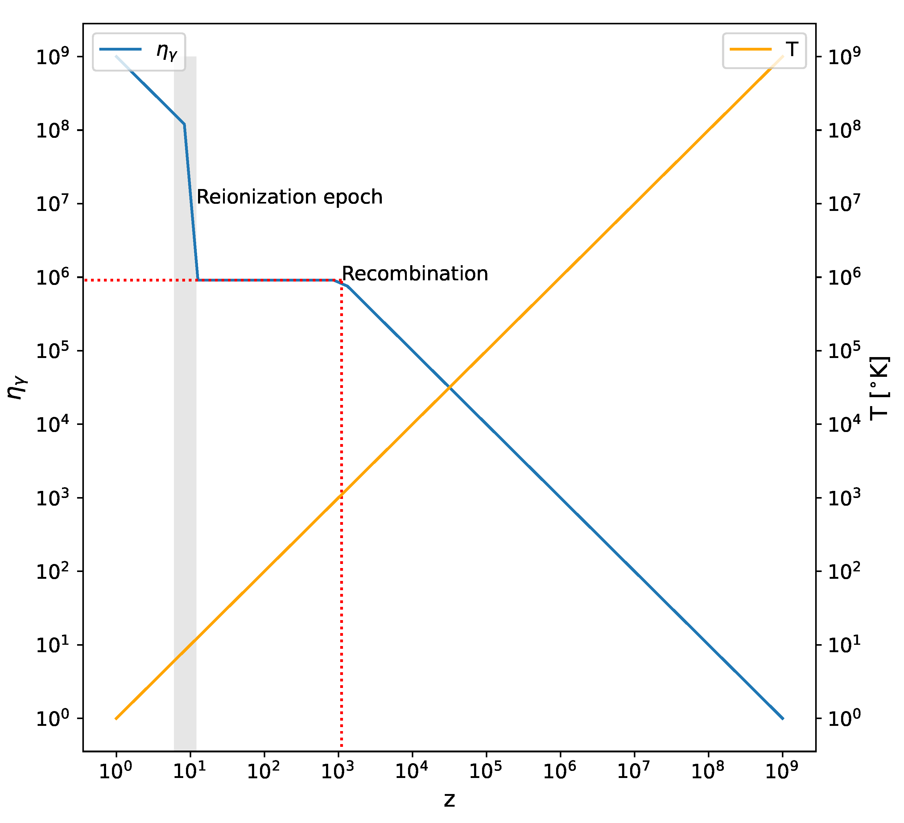
Figure 2.
Schwarzchild metric
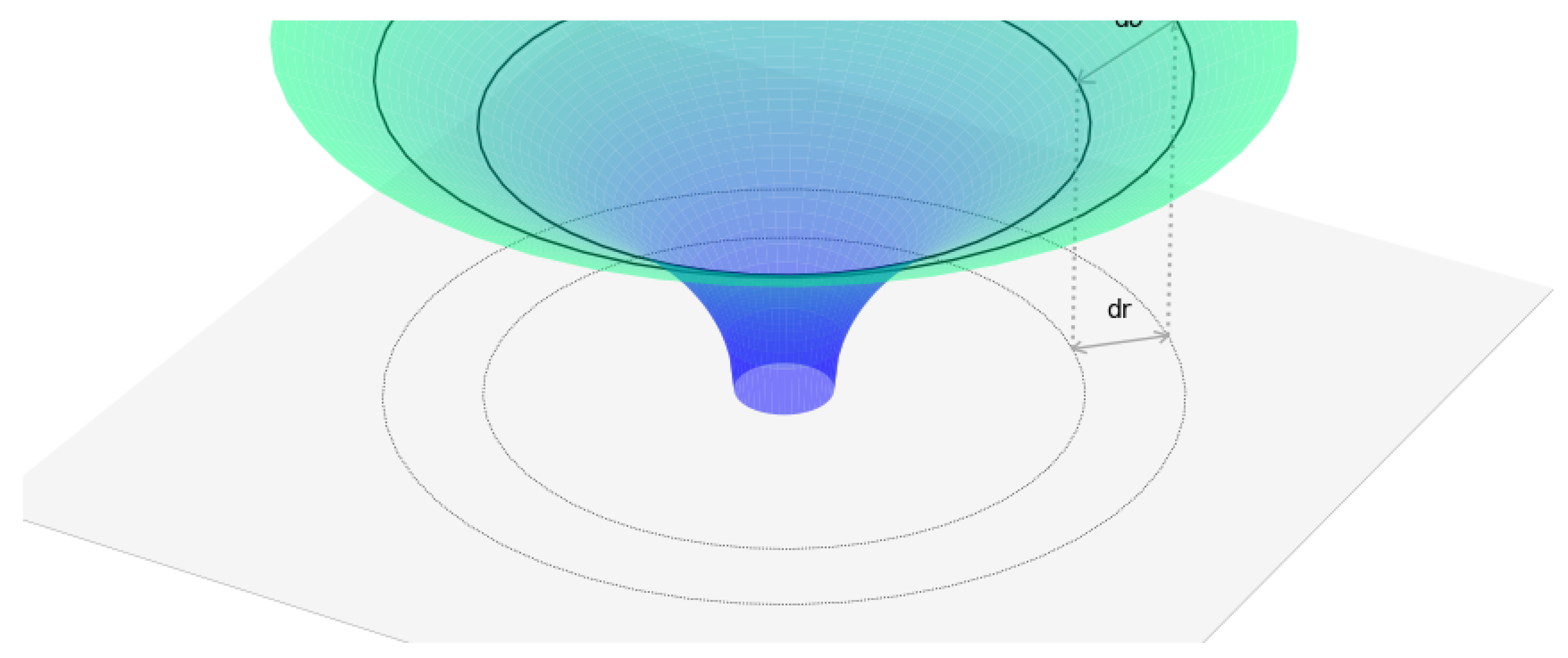
Figure 3.
Matter contraction in the Schwarzchild metric (This figure can be visualised as an animation if viewed in a PDF reader application.)
Figure 3.
Matter contraction in the Schwarzchild metric (This figure can be visualised as an animation if viewed in a PDF reader application.)
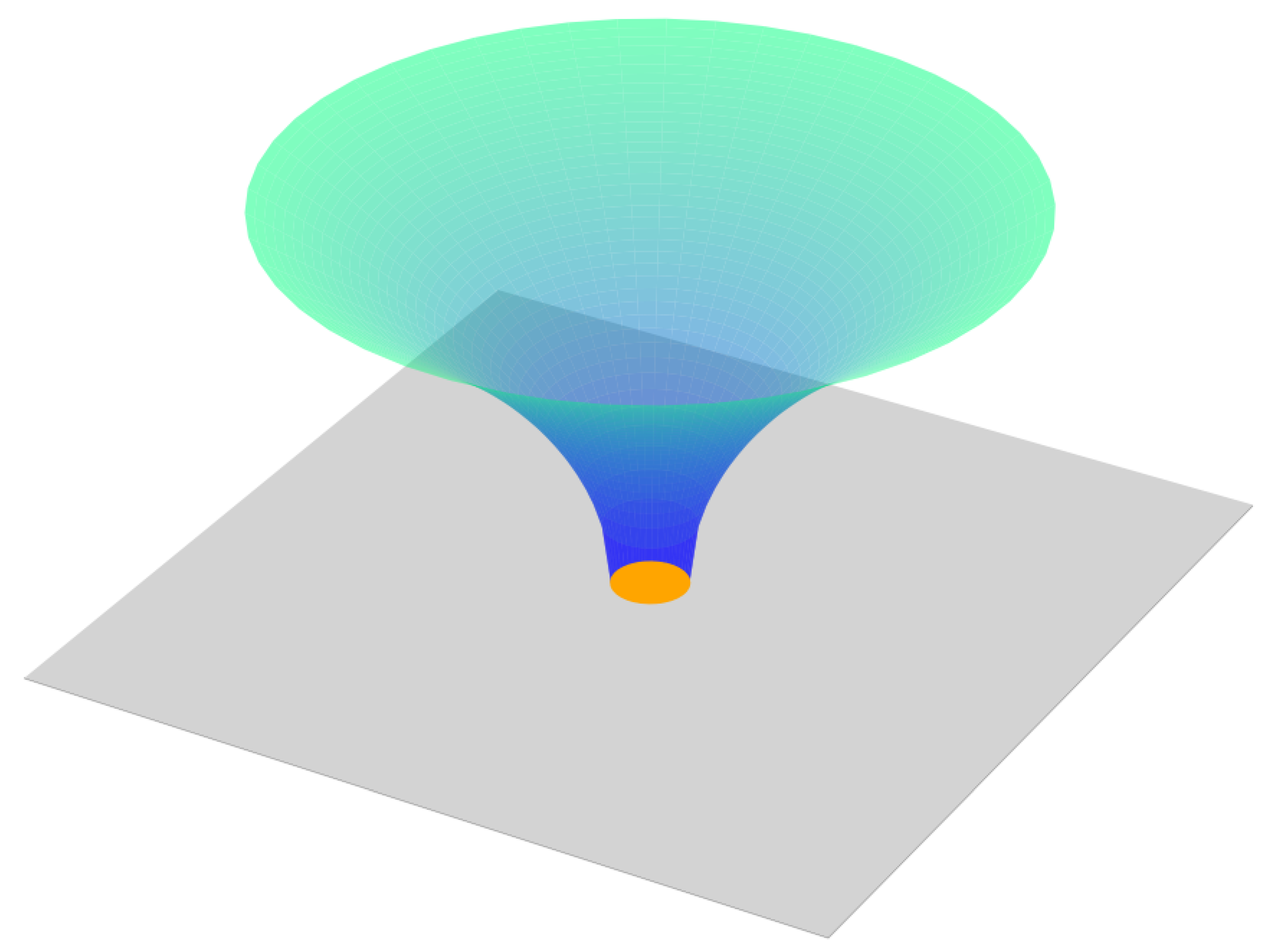
Figure 4.
Hubble parameter evolution as a function of redshift
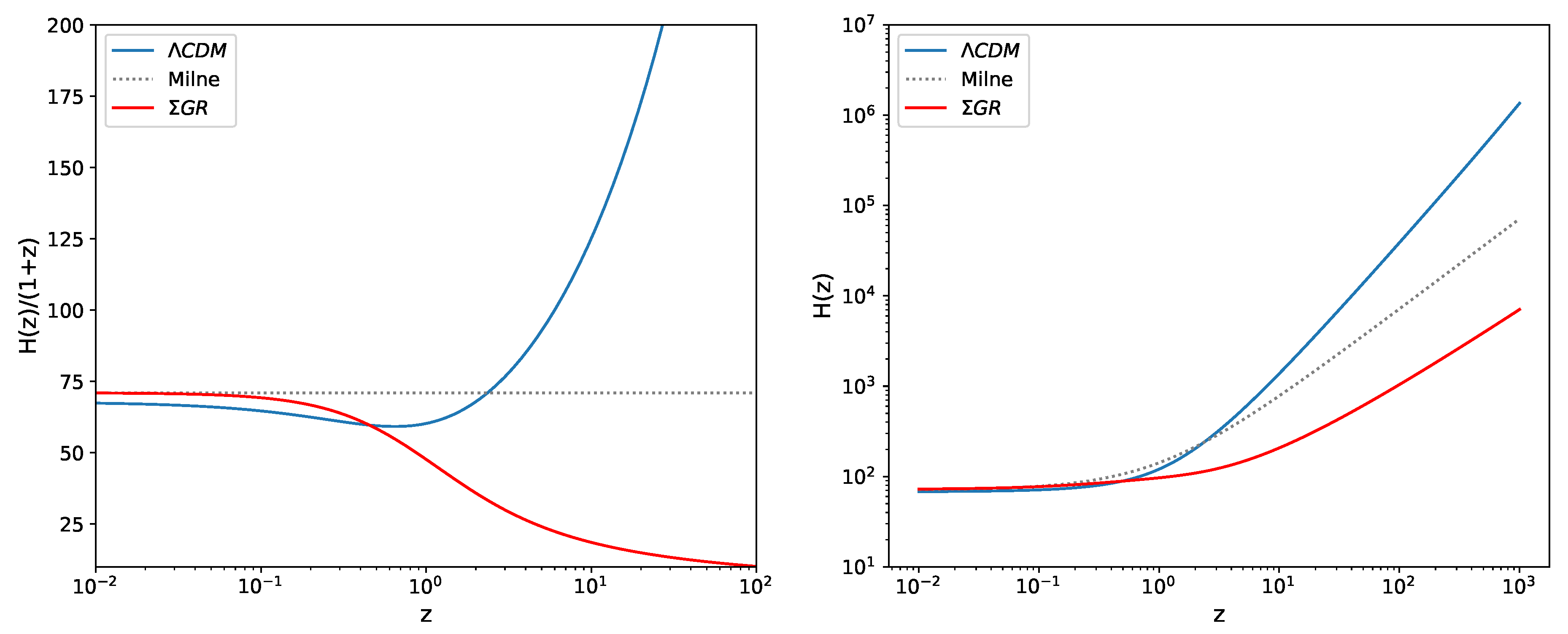
Figure 5.
Redshift-distance relations for different cosmological models
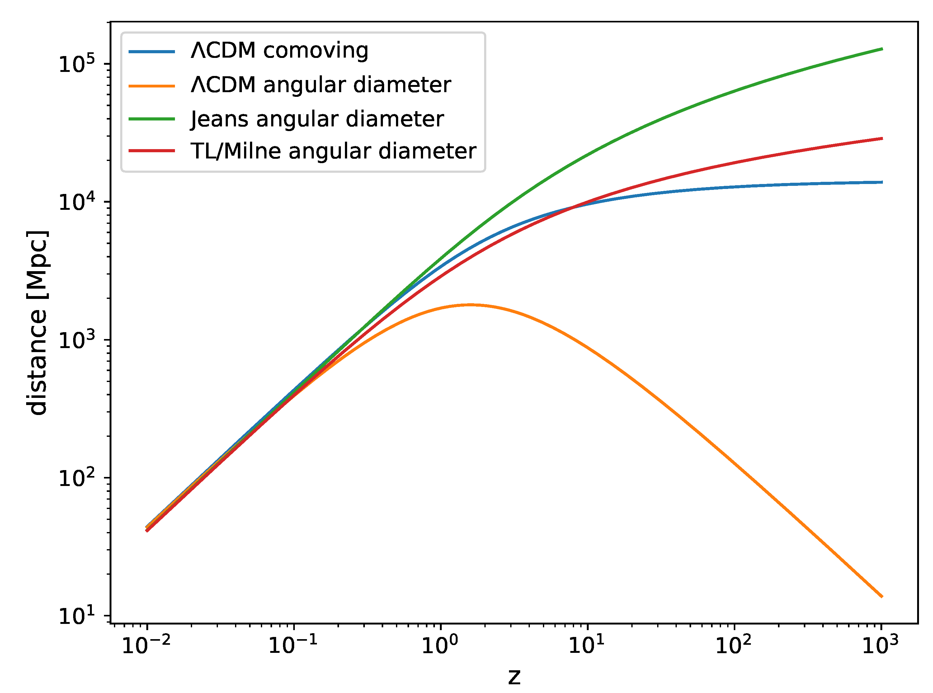
Figure 6.
Angular diameter as a function of redshift z for an object of fixed size .
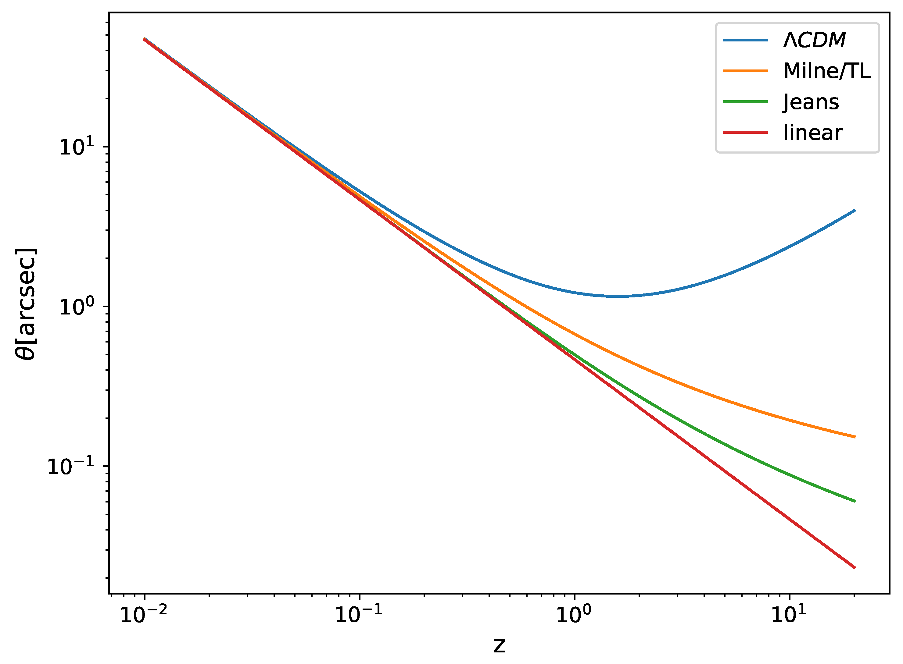
Figure 7.
Age - redshift relation
Disclaimer/Publisher’s Note: The statements, opinions and data contained in all publications are solely those of the individual author(s) and contributor(s) and not of MDPI and/or the editor(s). MDPI and/or the editor(s) disclaim responsibility for any injury to people or property resulting from any ideas, methods, instructions or products referred to in the content. |
© 2024 by the authors. Licensee MDPI, Basel, Switzerland. This article is an open access article distributed under the terms and conditions of the Creative Commons Attribution (CC BY) license (http://creativecommons.org/licenses/by/4.0/).
Copyright: This open access article is published under a Creative Commons CC BY 4.0 license, which permit the free download, distribution, and reuse, provided that the author and preprint are cited in any reuse.


