
Submitted:
05 December 2024
Posted:
06 December 2024
You are already at the latest version
Abstract
Retrofitting regional turboprop aircraft with hydrogen (H2)-electric powertrains, using fuel cell systems (FCS), has gained interest in the last decade. This type of powertrain eliminates CO2, NOx, and fine particle emissions during flight, as FCS only emit water. In this context, the "Hydrogen Aircraft Powertrain and Storage Solutions" (HAPSS) project targets the development of a H2-electric propulsion system for retrofitting Dash 8-300 series aircraft. The purpose of the study described in this paper is to analyze the performance of the retrofitted H2-electric aircraft during critical operating conditions. Takeoff as well as climb, cruise and go-around performances are addressed. The NLR in-house tool MASS (Mission, Aircraft and Systems Simulation) was used for the performance analyses. The results show that the retrofitted H2-electric aircraft has a slightly increased takeoff distance compared to the Dash 8-300 and it requires a maximum rated shaft power of 1.9 MW per propeller. A total rated FCS output power of 3.1 MW is sufficient to satisfy the takeoff requirements, at the cost of lower cruise altitude and reduced cruise speed as compared to the Dash 8-300. Furthermore, a higher rated FCS is required to achieve the climb performance required for the typical climb profile of the Dash 8-300.
Keywords:
hydrogen-powered aircraft
; hydrogen-electric propulsion
; retrofitted aircraft
; fuel cell systems
; performance analysis
; mission simulation
; powertrains
1. Introduction
Reducing greenhouse gas emissions and energy consumption is one of the main challenges for the development of future commercial aircraft. Design efforts to create aircraft with lower energy consumption – e.g. by weight reduction, improved aerodynamic efficiency and more efficient engines - are common in commercial aircraft development. The lower energy consumption also contributes to a reduction of the emissions. However, if kerosene is used as fuel, still CO2 and other greenhouse gasses are emitted during flight.
In the last decade also alternative fuels and propulsion systems have gained more attention in order to further reduce the environmental impact of aviation. For instance battery or hybrid electric powertrains, hydrogen (H2) powered propulsion or the use of sustainable aviation fuels (SAF) are being considered. The development of H2 powered aircraft has recently become a topic of major interest as it presents the opportunity to eliminate CO2 emissions. H2 for propulsion cannot be used in current transport aircraft, e.g. because of the absence of adequate H2 storage systems. Disruptive technologies to enable H2-powered aircraft are investigated in the European research programs Clean Aviation [1] and Clean Hydrogen [2]. In particular the onboard use of liquid hydrogen (LH2) is under investigation, taking advantage of its more compact storage potential in comparison to compressed gaseous hydrogen (GH2).
Novel aircraft propulsion concepts are being studied (and developed) either with H2 combustion engines, H2 fuel cells delivering electric power for electrically driven propulsors, or a combination of both [3,4,5,6,7,8,9,10] . In 2020, a feasibility study was performed [3] highlighting the potential of H2 in aviation and recommending further research in this direction. Various aircraft sizes were conceptually assessed, ranging from small regional aircraft with fuel cell based propulsion to large aircraft with H2 combustion. Several (more detailed) studies followed, addressing various aircraft sizes. Besides the aforementioned European research programs, aircraft concepts with H2 powered propulsion are being investigated by Airbus [4] and in several national research initiatives [5,6,7,8].
This paper addresses aircraft propulsion by means of fuel cells, in combination with electrically driven propellers: H2-electric propulsion. This type of propulsion provides opportunities to eliminate CO2, NOX, and fine particle emissions, as fuel cells only emit water. It also facilitates distributed propulsion layouts (e.g. [4,6,7]) which may have several advantages, such as improved aerodynamic and propulsive efficiency, system redundancy and steering by thrust vectoring [9]. In the aviation sector, H2-electric propulsion is a technology under development, and it poses several design challenges [10]. For example, difficulties arise for the H2 storage and distribution on board the aircraft due to the unique properties of the fluid and the stringent requirements in terms of safety, weight, and volume. The added weight, volume and packaging of the LH2 tanks result in weight and drag penalties to the aircraft design. Furthermore, fuel cells need special systems for conditioned air and H2 supply and they need an extensive cooling system. These additional systems also result in weight, volume, drag and power penalties which impact the aircraft design.
H2-electric propulsion is mostly investigated in the context of regional turboprop aircraft (e.g. below 2000 km range) [3,4,5,6,7]. In comparison to the relatively small gas turbines that are employed in regional turboprop aircraft, H2-electric propulsion systems (HPS) 1 can result in a higher overall efficiency of the powertrain [3,11]. Although regional aircraft are only a small fraction of the global aviation and will therefore have a limited climate impact, the development and maturation of the H2 technology for these aircraft may serve as stepping stone for application in larger aircraft [11].
H2-electric propulsion can either be applied to new aircraft concepts based on clean sheet design [4], or to retrofit existing aircraft [12,13]. In the case of clean sheet design aircraft, it is expected that these designs result in optimal performances, taking advantage of the benefits of a larger design space. Retrofitted aircraft have a smaller design space – being restricted by the limitations of the reference aircraft – and may therefore result in suboptimal performance. However, it is foreseen that certification efforts are less, resulting in a shorter time to market [13]. Several start-ups and established aircraft manufacturers have announced plans to develop fuel cell electric aircraft, or have even demonstrated retrofits of existing aircraft [10,14].
In the Netherlands, the " Luchtvaart in Transitie" (Aviation in Transition) program [8] has been established as a pioneering initiative to accelerate sustainability in aviation. Participating partners from the Dutch aviation sector are focused on developing innovative solutions, including energy-efficient technologies, lightweight materials and systems, and carbon-neutral propulsion systems, such as H2 powertrains. In this framework, the "Hydrogen Aircraft Powertrain and Storage Solutions" (HAPSS) project, launched in October 2022 [13,15], concerns the development of commercially viable HAPSS. The objective is to bring this technology to market by the end of the decade, starting from retrofitting of existing regional aircraft. The HAPSS comprise the powertrain from a LH2 tank to Fuel Cell System (FCS), electric motor and propeller, with all required auxiliary systems: thermal management, controls, and electric distribution. Figure 1 illustrates the aircraft concept proposed in the HAPSS project. The first case study is the De Havilland Canada Dash 8-300 series aircraft. This regional turboprop aircraft has a 50-passenger capacity. The proposed retrofit approach involves making a limited change to an aircraft that has already been certified.
Knowledge about the performance and sizing of HPS, i.e. what operating conditions constrain the design, is still under development [10]. For example, it is yet unclear which design point (takeoff, top of climb, etc.) is critical for the sizing of the HPS and the thermal management system (TMS) for a regional airplane like the Dash 8-300. The objective of the work described in this paper, is to understand the performance of the HAPSS aircraft concept during critical mission conditions, i.e. the mission conditions which impact the sizing of the HPS and the TMS, and to compare the performance with the reference kerosene aircraft (the Dash 8-300).
Full mission simulations with the HAPSS aircraft – e.g. for payload and range performance analysis – as well as sizing and performance analysis of the LH2 storage and distribution system are not in scope of this paper. Such simulations have been performed already and can be found in Ref. [13]. Instead, this paper focuses on specific mission phases and operating conditions that can be critical for the sizing of the HPS and the TMS. Results from Ref. [13] were re-used in the study, e.g. in terms of the mass breakdown of the retrofitted aircraft.
This paper addresses following research questions:
- What power rating of the HPS is needed to fulfill the takeoff requirements, according to CS-25 [16], and what is the corresponding takeoff distance?
- What is the impact on the TMS, in terms of cooling demand during takeoff?
- What power rating of the HPS is needed to fulfill the go-around (missed approach) requirements, according to CS-25 [16],
- What are the climb and cruise performances of the HAPSS aircraft for various HPS ratings and operating conditions?
The remainder of this paper is structured as follows. Section 2 describes the applied methods and developed models to simulate the performance of the reference aircraft and the HAPSS aircraft for various mission conditions. In Section 3 the performance simulation results are presented for the various mission phases and operating conditions. In Section 4 the simulation results are discussed, in relation to the model assumptions. Items for further research are identified. Section 5 provides a summary of the findings and concluding remarks.
2. Materials and Methods
This section contains the description of the applied methods, models, parameter settings and assumptions to carry out the mission performance simulations. First, the aircraft level assumptions are described (applied reference aircraft data and assumptions for the retrofitted H2-electric aircraft). Second, the tooling is described including the underlying performance models. These include the mission models, aircraft equations of motion, aerodynamic models, propeller model, engine model (for the reference aircraft) and HPS model (including the FCS and electric components, for the H2-electric aircraft). Models of the LH2 fuel system are not in the scope of this paper (as explained in the previous section). Fixed aircraft mass assumptions are applied, based on Ref. [13].
2.1. Aircraft Level Assumptions
The 311 model of the Dash 8-300 aircraft was selected as the reference aircraft to retrofit a turboprop aircraft with a H2 fuel cell system [13]. Key parameters of the reference aircraft which are used in this study are summarized in Table 1, while an illustration of the aircraft is provided in Figure 2. These parameters serve as a baseline for the performance simulations of both the reference and the retrofitted aircraft.
Some of the mass parameters in Table 1 are adapted for the retrofitted H2-electric aircraft (also referred to as the HAPSS aircraft). The sizing of the HAPSS aircraft is described in Ref. [13]. From this sizing process, the resulting aircraft mass breakdown is adopted:
- The aircraft operational empty mass (OEM) was increased from 11.6 t to 15.6 t, for the HAPSS aircraft. This increase is due to the additional HPS and LH2 fuel system masses (including tanks) [13].
- The maximum takeoff mass (MTOM) is lowered to the maximum landing mass of the reference aircraft (19.1 t). The reason for this decrease is that it is foreseen that the HAPSS aircraft cannot dump any fuel, after takeoff, in case of emergency [13].
- Due to the increased OEM and decreased MTOM, the payload mass is decreased to 3.1 t and the range is lowered to 750 km [13].
2.2. Mission Models
2.2.1. Mission Performance Tooling
The aircraft modelling and corresponding performance analysis was carried out using the NLR in-house tool MASS (Mission, Aircraft and Systems Simulation for energy performance analysis [21]). MASS is a MATLAB-based tool for mission performance and sizing analysis of aircraft and powertrains. Various aircraft powertrain configurations can be simulated, e.g. conventional turboprop, (hybrid) electric or H2-electric. System models of various complexity levels can be applied. The system models used in this paper are described in the following sections. With MASS, usually the fuel flow and total power are calculated as function of mission time in order to predict total trip fuel, energy consumption and emissions [11]. This is illustrated by the black arrows in Figure 3. The mission profile is then derived by interpolation between specified speed, altitude and rate of climb (ROC) combinations, which can be retrieved from public sources such as [22,23] as illustrated in Figure 4.
For specific use cases - when power values are known and when more detailed (acceleration, speed and ROC) performances must be determined, during specified mission segments (e.g. takeoff, climb or go-around) - an alternative simulation method was implemented in MASS, illustrated by the orange arrows in Figure 3.
2.2.2. Modelling of the Takeoff Phase
The takeoff phase of an aircraft can be subdivided into several segments determined by flap, landing gear and power settings [16]. The segments are bounded by specific speed and altitude values. The subdivision of the takeoff phase is illustrated in Figure 5. Two scenarios are considered: all-engines-operative (AEO) and the one-engine-inoperative (OEI). The speeds that mark the segment bounds are:
- Initial speed v0. This is the start speed of the takeoff run, typically 0 m/s.
- Decision speed v1 In case an engine failure takes place below this speed, the aircraft must be able to break and come to a standstill before the end of the runway. When the aircraft has reached v1 it must be able to continue the takeoff with the other engine(s) that is/are still in operation.
- Rotation speed vR. At this speed the aircraft starts it rotation, by using the control surfaces.
- Liftoff speed vLOFF. At this speed the aircraft lifts off and its altitude increases with respect to the ground level.
- Obstacle clearance speed v2. The aircraft must have reached this speed when reaching 35 ft (10.7 m) altitude above the ground.
- Climb speed venroute. This is the indicated air speed for (the first part of) the climb phase.
International Standard Atmosphere (ISA) conditions are considered in the takeoff analysis, as well as a dry runway at sea level, non-icing conditions, no runway slope and no wind. In the takeoff modelling, flap and gear settings were also taken into account, as well as rolling friction and ground effect (see Section 2.3). In the OEI case, asymmetric rudder drag and propeller feathering drag were also modelled, as described in Section 2.4. Furthermore, part of the analysis was to verify that the altitude gradients during the second and fourth segment climb (see Figure 5) are above the specified values in CS-25.111 and CS-25.121 [16], namely 2.4% and 1.2% for the second segment and the fourth segment respectively, for aircraft with two engines.
2.3. Aircraft Equations of Motion
In the default simulation flow (see the black arrows in Figure 3), the aircraft model takes as input the flight path variables from the mission profile in combination with aircraft specific parameters (such as the aircraft mass, and lift and drag coefficients as function of flap and gear settings and Mach number) and calculates the required thrust as function of time. The model is based on a so-called “point mass” representation of the aircraft, see Figure 6. Both flight and on-ground behavior have been modelled, taking into account normal forces and rolling friction as well as dependency of the aerodynamic coefficients on flap and gear settings.
Only forward motion and flight path angle are included in the flight mission; turns and maneuvers and roll and yaw rotations are not considered. The equations below detail the calculation process of the thrust , with all variables dependent on time t. SI-units are applicable. Changes in flight path angle γ are approximated by (piecewise) circular motion (see Eq. 7).
where v is true air speed (TAS), h is altitude, g is gravitational acceleration, L is lift force and m is aircraft instantaneous mass , which is calculated by
where is the takeoff mass and is the fuel flow which is computed using the engine or HPS model (see Section 2.6 and Section 2.7).
The drag forces D and Dground are calculated by
where is air density, is total wing area (reference area), N is normal force (N=0 N in the air) and µ is ground rolling friction coefficient (assumed equal to 0.03 [24]).
where and are the aerodynamic lift and drag coefficients, the lift coefficient at zero angle of attack (assumed equal to 0.12) and the zero-lift drag coefficient, the drag coefficients dependent on flaps, gear and OEI settings (rudder drag to stabilize the aircraft during the OEI case and propeller feathering drag due to the inactive propeller of the failed engine) respectively, and k the lift-induced drag coefficient. The time derivatives , and are approximated numerically.
If the alternative simulation model flow is chosen (see the orange arrows in Figure 3), the thrust is specified in the equations of motion. The specified thrust on its turn is calculated from the specified shaft power value using the propeller performance model, which is described in Section 2.5. The accelerations and flightpath angle are calculated in a segmented approach. During the horizontal flight segments – e.g. takeoff ground run - the flightpath angle is set to zero. The acceleration is calculated by modifying Eq. 1 to
and calculating by time integration of
During the non-horizontal flight sections the flightpath angle is calculated by rewriting Eq. 1 to
In this case either a constant velocity is assumed (zero acceleration) or the velocity is interpolated linearly with altitude and is then approximated numerically from . The altitude is calculated by time integration of combined with Eq. 2
In all cases the horizontal distance is calculated by time integration of the horizontal velocity by
2.4. Aerodynamic Coefficients
The aerodynamic coefficients of the aircraft lift-drag polar – as used in Eq. 9 - were estimated by comparing information from various sources from the public domain. Drag polars from an ATR 42 related study by Gunnam [25], a Dash 8-300 related study by Quillet et al [26] and from conceptual design textbooks Roskam averaged statistics [27] and a combination of Roskam and Obert [28] were compared. The coefficients – for the clean configuration without flap or gear contributions - are summarized in Table 2 below. The corresponding drag polars, depicted as lift-to-drag ratio as function of lift coefficient are shown in Figure 7.
Figure 7 shows that the various drag polars have similar shapes but the one provided by Quillet [26] has the lowest L/D prediction. In the remainder of this study, this polar was applied, following a worst case estimation approach. Because the drag contributions of flaps and landing gear were not provided in Ref. [26], the estimations provided by Roskam [27] were applied. The resulting coefficients for the clean and for the takeoff condition are summarized in Table 3 below.
In the OEI case, the rudder must be deflected to stabilize the aircraft forward motion due to asymmetric thrust by the one engine that is still in operation. This creates additional drag. The “asymmetric rudder drag” contribution was estimated 3 by the empirical relation
with the rudder deflection in radials. A maximum value of 16 deg (0.28 rad) [29] was applied, which leads to a contribution of 0.0055. Furthermore, in the OEI case, the dysfunctional propeller will feather but still cause additional drag. To estimate the additional drag, a formula by Torenbeek [30] is used
where is the wing surface area, Bp the number of propeller blades and Dp the propeller diameter. Applying the values from Table 1 results in a of 0.0014.
As the takeoff is performed in close proximity of the ground, the ground effect is taken into account for performance calculations. The effects are expressed as ratios between, on one hand the lift coefficient in ground effect () with respect to the lift coefficient in the absence of the ground effect (), and on the other hand, the ratio between the lift-induced drag factor in ground effect (keff) and the lift-induced drag factor in absence of the ground effect (k). The ground effect on the lift coefficient is expressed using the ratio by Torenbeek [30]. The formula is simplified by assuming a straight wing (without sweep):
where h is the distance between the wing and the ground (for this purpose assumed to be similar as the modelled altitude), cg is the mean geometric chord of the wing, Bw is the wing span, AR is the wing aspect ratio, is the ground effect factor, a correction factor for the ground effect and is the lift curve slope obtained from the thin airfoil theory formula, which are obtained from:
The ground effect on the drag coefficient is determined using the method by Raymer [31], for which the lift induced drag term – see also Eq. 9 - is corrected with the factor .
Eq. 17-22 show that when the altitude h becomes sufficiently large, the ratios and get closer to 1.
Finally, as explained in Section 1, the HPS is retrofitted into the Dash 8-300 aircraft. Therefore, the aerodynamic coefficients that are applicable to the reference aircraft are also applicable to the H2-electric configuration. Nevertheless, additional drag is expected from an increased nacelle size, and from the ram air ducts that are needed to cool the fuel cells. Detailed drag models were not available yet, due to the conceptual stage of the design. Instead a rough estimation was made that the increased wetted surface of the nacelles and ram air drag of the TMS would lead to overall increase of the parasite drag coefficient with 7% [32].
2.5. Propeller Model
The thrust that is needed for the aircraft motion (see Eq. 1) is delivered by a propeller. In case of the Dash 8-300 it is a Hamilton Sunstrand propeller with four blades, variable pitch and a maximum propeller shaft speed of 1212 rpm [19]. The relation between thrust and propeller shaft power was modelled by
where v is the true air speed, the total net thrust, the total mechanical shaft power and the propeller efficiency.
The propeller efficiency was modelled by reproducing the Dash 8-300 propeller map presented in Ref. [26]. In the propeller map the propeller efficiency is given as function of advance ratio J and power coefficient , by
where is the air density in kg/m3, n is the shaft speed in rev/s, is the propeller diameter in m and is the lookup table interpolation function as illustrated in Figure 8.
For situations where shaft power should be computed for a known thrust, a second propeller map is constructed which gives the propeller efficiency as a function of advance ratio J and thrust coefficient , by
where is the lookup table interpolation function as illustrated in Figure 9.
2.6. Engine Model
In the reference aircraft the shaft power is delivered by a PW123 turboprop engine. A maximum shaft power of 1775 kW per engine can be provided [20].
The engine model depicted in Figure 3 was used to predict fuel flow as function of shaft power and flight conditions. The fuel flow (used in Eq. 3) can be predicted by means of the Power Specific Fuel Consumption (PSFC) number
The PSFC depends on the actual flight condition. For the PW123 engine a PSFC during takeoff of 0.286 kg/kWh was found [33]. The PSFC values in the other flight phases were modelled by using an in-house data set of a similar turboprop engine and scaling it with the takeoff PSFC value. Typical values are listed in Table 4.
2.7. HPS Model
In the simulations with the HPS retrofitted aircraft, the gas turbine engine model was replaced by an electric propulsion unit (EPU) and FCS performance model. The applied models are described in Section 2.7.1 and Section 2.7.2.
The EPU and FCS are connected by an electric (DC) distribution system. Figure 10 depicts the applied architecture of the HPS, in a simplified way. The EPUs of the two propeller shafts are powered by four FCS modules. The DC busses of the EPUs are cross-connected: if one FCS module fails, the other three can still provide power and divide it over the two shafts.
In Ref. [13] also batteries are considered as part of the system architecture, e.g. to provide transient power demands. In our study they were not modelled, as transient system responses were not considered.
2.7.1. EPU Model
The EPU [13] consists of the electric motor (EM), inverter and reduction gearbox (RGB) and delivers shaft power to the propeller. The EPU model describes the power losses by means of efficiencies. Also electric power losses in the electric distribution system (e.g. cables and DC-DC converters) are included. Furthermore the power offtakes needed for the non-propulsive systems (e.g. ice protection system, environmental control system, flight controls, avionics) are taken into account. For simplicity, all these losses and the power offtakes are embedded in the EPU model. The model describes the relation between propeller shaft power to be delivered and the corresponding electric DC power demand to be delivered by the FCS:
where - estimated at 88% - represents the multiplied efficiencies taking into account the power losses at the RGB, motor, inverter and electric distribution system. represents the power needed for the offtakes, which ranges between 1% and 4% of the shaft power, depending on the flight phase [13].
2.7.2. Fuel Cell System Model
The FCS consists of the fuel cell (FC) stack and balance of plant (BoP) components. The FC stack generates the electric power (by means of oxidation of supplied H2). The BoP components are needed to provide the optimal operating conditions of the fuel cell stack in terms of air supply mass flow, pressure, temperature and humidity. Furthermore the FC stack must be cooled. In our FCS model, the considered BoP components are:
- a compressor that is needed to deliver the air mass flow, at the pressure needed by the FC stack;
- a heat exchanger to lower the air temperature – which increases due to the compressor – to the temperature level needed by the FC stack;
- a humidifier that creates the level of air humidity needed by the FC stack.
The power consumption of the TMS that cools away all heat generated by the FCS components is addressed as well. The FCS model is shown schematically in Figure 11.
The FCS model describes the relation between DC output power and H2 fuel flow
where represents the overall FCS efficiency and represents the Lower Heating Value of H2 (120 MJ/kg).
and cannot be computed directly for a desired , but can be computed for a given , the FC stack output. Rather than employing an iterative method to find the that leads to the desired , values of , and are pre-computed for a range of values, and the results are interpolated.
The FC stack model was based on measurement data from an ElringKlinger fuel cell [34]. This data, valid for a stoichiometry factor of 1.7, was reworked into a map relating FC stack pressure and power density pd to cell voltage , shown in Figure 12, and a relation between pressure and fuel stack temperature , shown in Figure 13. Power density pd is defined as
where is the total area of the cells. The efficiency of the fuel cell (for the LHV) and the fuel consumption follow from Ref. [35]:
where is the cell reference voltage of 1.25 V [35].
It was assumed that the compressor will be electrically driven and use a (small) part of the electric power delivered by the FC stack. The compressor power depends on the FC stack pressure and the pressure losses in the air filter, heat exchanger and the humidifier. is a model parameter and is assumed constant throughout the mission. The pressure losses for various components that were assumed are specified in Table 5. The compressor power was modelled (in a simplified way) by
where represents the air mass flow (derived from the H2 fuel flow and stoichiometry factor), the specific heat capacity, the ratio of the specific heat capacities, the isentropic efficiency and the driver efficiency (motor bearings etc.). The values used can be found in Table 5. and represent the total temperature at the compressor inlet and outlet respectively, and PR represents the compressor pressure ratio. As a simplification, the ram air compression effect in the FC stack air intake was ignored, and the compressor is used for the compression from static ambient ISA atmosphere temperature ( and pressure () to the required pressure. This simplification (conservatively) overestimates the required compressor power, especially at higher Mach numbers 4, but it eliminates the dependency of the FCS model on flight velocity, greatly reducing the number of iterations (computational cost) needed to create the lookup tables for interpolation.
The heat exchanger model – describing heat to be cooled away from the compressed air – is shown below in Eq. 39. Furthermore a fixed pressure drop was assumed for the heat exchanger (see Table 5).
For the humidifier only a fixed pressure drop was modelled (see Table 5). The air humidity itself is not taken into account in this FCS model.
The TMS coolant pump power (PTMS), needed to cool the FCS components is modelled as follows. First, the total FCS heat flux to be cooled away is computed as the sum of the heat fluxes generated by the FC stack (), by the heat exchanger cooling the air () and by the electric motor that drives the compressor ():
is modelled as 2% of the heat flux to be cooled away, based on inhouse experience. Note that the drag of the TMS ram air ducts is accounted for in the aerodynamic model (see Section 2.4). The residual thrust from the exhaust is ignored and the potential for power recovery with a turbine is not considered in this study.
Finally, the FCS output power follows from
The fuel stack design, including the design pressure, is outside the scope of this work. Typical operating pressures lie in range of 1.6 bar(a) to 1.9 bar(a) [36]. A fuel stack pressure of 1.6 bar(a) was assumed in the simulations in this paper.
No compressor speed limit is applied in the compressor model, while it is known to greatly affect the maximum achievable FCS power at altitude. To incorporate this effect, the maximum system power as function of altitude found by Ref. [34] is added as a limit to the model. This limit is shown in Figure 14.
Figure 14 depicts the derived FCS efficiency model, as function of altitude and FCS output power, relative to rated FCS output power. This refers to the maximum net useful (DC) output power of the FCS, at sea level ISA conditions, at the “end-of-life” condition. BoP power losses (e.g. compressor power) are already subtracted, see Eq. 41. Figure 14 shows that the overall FCS efficiency decreases with altitude and with power demand.
3. Results
The section presents the results of the performance simulations during critical mission phases. The first part describes the takeoff performance results. In the second part the performance during climb, cruise and go-around is described.
3.1. Takeoff Performance
In this section only the takeoff conditions for the OEI cases are presented as these cases represent the critical performances.
3.1.1. Validation with Reference Aircraft Data
As a first step, takeoff simulations were performed with the reference aircraft model, for comparison with reference data. In Ref. [17] information on takeoff distances (TOD) was found for the reference aircraft. A takeoff with OEI was simulated: when the aircraft has reached decision speed v1, one engine fails and the takeoff is proceeded in the OEI condition. The TOD represents the distance from takeoff start to the point where the 35 ft (10.7 m) clearance altitude is reached, see also Figure 5. A dry runway, non-icing conditions, no runway slope and no wind are applicable. ISA sea level conditions were used. Figure 15 shows the results for the TOD segment. The simulation starts with normal takeoff (NTO) power of ~1600 kW per engine which adds to ~3200 kW in total [20]. After the engine failure at v1 the remaining operating engine is switched to a maximum takeoff (MTO) power setting (1775 kW). This results in a TOD of 1767 m. This simulation was performed with a takeoff mass (TOM) of 19.5t, which is the maximum TOM of the reference aircraft (see Table 1). The simulation was repeated for various TOM values. The resulting predicted TOD values, were compared with the corresponding data in Ref. [17]. The comparison results are shown in Figure 16. It can be seen in Figure 16 that for the lower TOM values the simulated TODs match well with the data from [17]. For the larger TOM values the simulation predictions overestimate the TOD data, up to 11%.
3.1.2. HAPSS Aircraft Results
Second, the takeoff phase (with OEI) was simulated with the HAPSS aircraft model, under the same conditions as with the reference aircraft (ISA, dry runway etc.). The TOM was reduced from 19.5 t to 19.1 t (following the assumptions in Section 2.1). The parasite drag coefficient of the aircraft increases with 7% (see Section 2.4). From Figure 10 it can be deduced that the most critical failure of a single component is the case where one propeller (or EPU) fails, rather than one FCS module. In that case only the maximum shaft power that is allowed by the other propeller can be used. The propeller failure is therefore considered the OEI case for the HAPSS aircraft. Initially the same MTO shaft power as with the reference aircraft was applied: 1775 kW. Figure 17 shows that this MTO power is not sufficient to achieve the 2.4% gradient requirement [16] during the second segment climb. At least an MTO shaft power of 1865 kW is needed to fulfill this requirement. Figure 17 also shows that both MTO power levels are more than sufficient to achieve the 1.2% gradient requirement [16] during the fourth segment climb. It should be noted that the MTO power was maintained until the end of the takeoff phase. For the HPS there are no time restrictions to maintain maximum power. However, in case of the reference aircraft MTO power to be provided by the engine would be time restricted [20] and therefore the fourth segment climb would be performed with a (lower) maximum continuous (MCT) power setting, as specified in Figure 5.
Figure 18 zooms in on the first part of the takeoff phase – until the 35 ft (10.7 m) clearance altitude is reached – and shows that a TOD of 1838 m and 1717 m can be achieved with the 1775 kW and 1865 kW MTO power settings respectively.
This takeoff simulation was performed with a total rated FCS (output) power of 3.1 MW (see Section 2.7.2). This results in a total available propeller shaft power of 2.7 MW, during the first part of the takeoff, when both propellers are still in operation, as can be seen in Figure 17. After the propeller failure it is assumed that at least one FCS module on this propeller side is still operative and can provide electric power to the other side, facilitated by the cross-connected DC busses (see Figure 10).
3.1.3. Sensitivity Analysis of HAPSS Aircraft Parameters
The performance model still contains many uncertainties because several parameter were estimated, such as the parasite drag coefficient , induced drag coefficient k, ground roll friction coefficient and the propeller efficiency . Therefore a sensitivity analysis was applied to better understand their impact on the predicted TOD and second segment climb gradient (in case of OEI). In addition, the takeoff speed values (v1, vR, vLOFF, v2 ) were varied to estimate their impact on the takeoff distance and second segment climb gradient. For all parameters deviations from the reference values were applied, from - 10% to +10% (except for the propeller efficiency which has -5% as lower bound 5), in separate cases. Quadratic polynomials were fitted to the lower, upper bound and reference values, to predict the sensitivity behavior in between the bounds for each parameter. The results are depicted in Figure 19. The propeller efficiency has largest impact (both on TOD and second segment gradient). The induced drag factor k has the second largest impact, has third largest impact. Increased velocities (v1, vR, vLOFF, v2) have large impact on TOD but a small impact on the gradient.
3.1.4. Effect of Gradual Power Increase on Fuel Cell Cooling Demand
During the takeoff analyses full NTO power was applied, immediately from the start of the takeoff phase (see the bottom plots of Figure 17 and Figure 18). Applying full FCS power at the beginning of takeoff can be very demanding for the cooling of the FC stack, due to the low air speed. Therefore, the effect of gradually increasing the power from the start of the takeoff, was also investigated, see Figure 20.
The FCS power was increased from 20% to 100% of the maximum NTO power, reaching that maximum at different speeds: either at the start of takeoff (v0), at the ground minimum control speed (vMCG), at the air minimum control speed (vMCA) or at decision speed (v1 ). The impact on TOD - while applying the OEI condition after v1 was reached with MTO power 1865 kW - and fuel cell cooling demand was simulated. The latter is derived using Eq. 37 and shown in Figure 20. Table 6 summarizes the results, where the cooling demand was evaluated at the (arbitrary) speed of 40 kts (20.6 m/s). The cases with gradually increased power reduce the cooling demand – at 40 kts - with at least 57% but result in an TOD increase of 9 to 21%.
The investigated cases have no effect on the second segment climb gradient, as in this segment the same MTO power setting is applied, similar to the previous takeoff analyses.
3.2. Performance During Other Mission Phases
3.2.1. Go-Around Performance
With a similar approach as with the takeoff analyses, the go-around (or missed approach) mission phase was analyzed. During the final approach phase, the aircraft switches to takeoff power settings, with OEI. During go-around, CS-25 [16] requires a minimum 2.1% climb gradient in the OEI case. Similar to the takeoff case, this value could be achieved with the 1865 kW shaft power (one propeller) but not with the 1775 kW shaft power, as is illustrated in Figure 21.
3.2.2. Climb Performance
Contrary to the takeoff phase, no hard requirements were available for the climb phase to determine the minimum required FCS rated power. Instead, the example mission ROC profile for the reference aircraft (see Figure 4, taken from Ref. [22]) was used to evaluate the maximum rate of climb of three HAPSS aircraft variants with different FCS size in Figure 22. The black dashed line depicts the example ROC profile, and serves as a reference.
The first selected FCS size (yellow curve in Figure 22) is identical to the FCS with 3.1 MW rated power, as determined in the previous section. This FCS can in theory fly to flight level (FL) 240 (24.000 ft, 7315 m altitude), but at a very slow climb rate 6. The second FCS -which has a larger rated power (4.2 MW, purple curve) and will therefore be larger and heavier - can follow the reference mission profile up to FL140 and is able to achieve a maximum climb rate of 500 ft/min at FL240, which is about half the climb speed at that altitude in the example mission profile. The third (even larger) FCS (5.5 MW, green curve) is able to follow the typical mission profile with a maximum climb rate of 1000 ft/min at FL240. This FCS is required for a comparable climb performance to the reference aircraft (dash-dotted blue line), in terms of maximum rate of climb at higher altitude.
3.2.3. Cruise Performance
Finally, the cruise performance of the HAPSS aircraft was analyzed. Using the 3.1 MW rated FCS, several cruise altitude and speed settings were varied, to explore the effect on the energy efficiency. Figure 23 illustrates the exploration results in terms of range specific energy consumption (RSEC) in MJ/km, and shows the range-optimal altitude 7 for each speed (marked by the red curve). For comparison also the same exploration was performed with the reference aircraft. The RSEC is calculated for each potential cruise altitude-speed combination, by dividing the cruise fuel flow by the corresponding air speed and multiplying it with the LHV. The RSEC is impacted by the aerodynamic efficiency (L/D), propeller efficiency and HPS efficiency (of the HAPSS aircraft) or gas turbine efficiency (of the reference aircraft). For the HAPSS aircraft, the RSEC increases with altitude, which is mainly caused by the increasing compressor power needed for the FCS. For the reference aircraft, it is the other way round: the gas turbine operates more efficiently at higher altitudes. For both aircraft the RSEC contours also show symmetry compared to the speed values. This is because L/D is optimal for a particular lift coefficient (as can be seen in Figure 7). The cruise lift coefficient on its turn is impacted by the speed and altitude (see Eq. 8).
Figure 23 also provides information on the operating limits. It shows that with the 3.1 MW rated FCS, cruising at the Dash 8-300 ceiling altitude of 25.000 ft (7620 m) with a TAS of 133 m/s (see Table 1) is not feasible 8. The FCS output power limit - included to represent the compressor speed limit (see Section 2.7.2) - causes the visible operating limits. Following the red line in the right part of Figure 23 shows that an optimal cruise performance (in terms of high range and high TAS) is achieved at 112 m/s and 5800 m. Larger TAS values are feasible, but due to the operating limits the HAPSS aircraft is forced to fly lower, which causes a decrease in L/D and therefore a sharp increase in RSEC. In general, following the red line in the right graph of Figure 23 shows that flying lower and slower decreases the RSEC, in the HAPSS aircraft case.
When comparing the left and right graph of Figure 23 one can see that the overall RSEC values of the HAPSS aircraft are lower. This can be explained by the differences in powertrain efficiency. The reference aircraft has a typical cruise PSFC of 0.284 kg/kWh (see Table 4) which corresponds to an overall powertrain efficiency (from fuel power to shaft power) of ~30%. The HAPSS aircraft has an FCS efficiency of ~47% at the maximum feasible operating power (see Figure 14). Taking into account the EPU losses, this results in an overall powertrain efficiency of ~42%. This efficiency increase still compensates the drag increase due to the TMS (estimated at 7% increase in ).
4. Discussion
In this section the results (see the previous section) are discussed in relation to the underlying models, methods and assumptions. Potential improvements and directions for future research are suggested.
In the results section it was shown that the performance models overestimate the TOD with 11% for the MTOM case of the reference aircraft. This overestimation could be (partly) due to the relatively “pessimistic” setting of the aerodynamic coefficients (see Section 2.4). The sensitivity analysis described in Section 3.1.3 shows that a 10% decrease in induced drag coefficient k results in ~5% lower TOD 9.
The TOD overestimation could also be (partly) explained by a (small) level of exhaust thrust that the gas turbine engine produces during takeoff [37], which could be implicit to the lower TOD values stated in Ref. [17], but which was not taken into account in the TOD simulation.
The values stated in Ref. [17] to which the simulated TOD were compared are in fact takeoff field length (TOFL) values. The TOFL [16] is the maximum of the TOD and the accelerate stop distance: the total distance needed to accelerate to v1 and then decelerate to full stop, in case the pilot chooses to reject the takeoff after engine failure. The accelerate-stop case was not simulated in this study. However, given that the TOD estimations in this paper - based on the OEI case only - already overestimate the reference values in Ref. [17] this was considered sufficient to proceed, following a worst case approach.
From Section 3.1.2 it was learned that, with the HAPSS aircraft, the TOD increases slightly w.r.t the reference aircraft, although the MTOM was reduced from 19.5 t to 19.1 t. This increase is caused by the additional drag. Furthermore, with an MTO power setting of 1775 kW – based on the rated MTO power of the reference aircraft - the 2.4% gradient requirement in the second segment climb could not be achieved. At least a MTO power of 1865 kW would be necessary. Given the worst case approach (as described above) this value could reduce, when more refined models are available. Nevertheless, a shaft power of 1865 kW seems feasible, as a maximum shaft torque of 14913 Nm and a maximum rotational speed of 1212 rpm could be applied [20], which results in 1893 kW maximum power. This remains to be checked for the exact propeller (sub)type to be applied for the HAPSS aircraft, during the subsequent design phases. For the FCS the 1865 kW is also not limiting as this power can be delivered easily, when at least three of the four FCS modules are in operation.
It was also found that a gradual increase of power at the first part of the takeoff phase reduces cooling demand drastically (more than 50% during the early takeoff phase), whereas it increases the TOD with 9 to 21%. The second segment climb gradient is not impacted by this gradual power increase.
The takeoff simulations were restricted to ISA (sea level) conditions, with a dry runway, no ice, no runway slope and no wind in accordance with Ref. [16]. Nevertheless, the current models can be extended to also simulate the other conditions, as part of future work.
The findings from Section 3.1 are also applicable to the go-around phase. The required MTO power needed for the takeoff phase was found to be sufficient for the OEI case in the go-around (or missed approach) phase, as described in Section 3.2.1.
In Section 3.1.3, it was already acknowledged that several model parameters are still subject to uncertainty. A more refined version of the drag polar could improve the takeoff performance simulations. Especially the estimation of the additional parasite drag of the HAPSS aircraft due to the increased wetted surface of the nacelles and ram air drag of the TMS was based on a rough estimation. Nevertheless, it was learned from the sensitivity analysis in Section 3.1.3 that changes to the parasite drag coefficient do affect the TOD and climb gradient, but changes to the induced lift coefficient k and especially the propeller efficiency have a larger impact. Therefore, further validation and improvements to the modelling of both the propeller and the aerodynamic coefficients is recommended for further work.
From the takeoff simulations it was learned that an FCS with 3.1 MW rated power would be sufficient to achieve the takeoff requirements, when taking into account that three out of four FCS modules will be always available, based on the electric architecture with cross connections between the two HPS nacelles (see Figure 10). If these cross connections are not feasible, the 1865 kW MTO shaft power needs to be provided by two FCS modules, which would result in a higher total FCS rated power. Also from the climb simulations in Section 3.2.2, it was learned that an 3.1 MW rated FCS has strong limitations on the climb performance (e.g. a climb time of at least one hour to FL240, making that altitude practically unfeasible). With a 4.2 MW rated FCS, an improved climb performance could be achieved. This higher rating will come with a volume and mass penalty and potentially a larger drag penalty. Nevertheless, a higher rated FCS can also provide more NTO power during the first part of the takeoff (which would result in a lower TOD) or it allows the FCS to operate with increased efficiency during the NTO phase. If the same power as with the lower-rated FCS is applied, this then requires a lower power fraction which results in an increased FCS efficiency (see also Figure 14). This efficiency increase reduces the cooling demand which could result in a smaller TMS (and therefore smaller nacelles). It is recommended to further study these potential effects as part of future work. Anyhow, if the lower rated FCS of 3.1 MW is applied, it is recommended to reduce the cruise altitude and speed, as is explained in Section 3.2.3.
It needs to be remarked though that the FCS performance simulations were based on simplified modelling. The stack operating pressure was based on a fixed value of 1.6 bar(a) but could be optimized [36]. The compressor was modelled with fixed efficiencies instead of performance maps. A speed limit of compressor was assumed indirectly, modelled as a power limit of the FCS (based on Ref. [34]), which strongly impacts the climb and cruise performance limits. Improved models of the compressor and of the air supply system (taking into account other designs and architectures) could be part of future work. The simplification of the FCS modelling has limited impact on the takeoff performance though as here the shaft power requirements were focused on. Nevertheless, improved models of the FCS will also impact the FCS cooling demand during takeoff. Part of these improvements could also be to model interaction between the TMS sizing and FCS sizing (during takeoff) and corresponding trade-offs, e.g. the relation between FCS operating temperature, efficiency, mass, heat capacity and TMS sizing.
Finally, the model enhancements could also include batteries, e.g. provide startup power and to reduce the FCS peak power demands, which could also result in a smaller TMS [13] (and therefore smaller nacelles).
5. Conclusions
A first version of the mission performance models has been created of the HAPSS modified Dash 8-300. The models were (partially) validated by comparing the reference aircraft predictions against available performance data.
The focus of this paper was on the performance in the takeoff, climb, cruise and go-around phases. From the analyses it follows that the HAPSS aircraft has a slightly increased TOD as compared to the reference aircraft and that it requires a MTO power of 1865 kW to satisfy the gradient requirement during the second segment climb during takeoff and during the go-around phase. It was also found that a gradual power ramp-up at the first part of the takeoff phase reduces cooling demand drastically (more than 50% during the early takeoff phase), whereas it increases the TOD (up to 21%). The second segment climb gradient is not impacted by this power ramp-up.
A total rated FCS power of 3.1 MW was found sufficient to satisfy the takeoff and go-around requirements, under the system architecture assumption that, if one propeller fails, the other propeller can receive power from at least three FCS modules. However, with this FCS sized for takeoff, the Dash 8-300 ceiling altitude of 25.000 ft (7620 m) and typical cruise speed of 133 m/s could not be achieved. The operationally optimal cruise point was found to be 5800 m altitude at 112 m/s. Furthermore, it was found that a higher-rated FCS will be needed to achieve a climb performance, that gets closer to the reference aircraft climb profile. A higher rated FCS may also allow for a lower cooling demand during takeoff, but it comes with mass and volume penalties and potentially drag penalties, which need to be further investigated as part of future work.
Finally, it should be remarked that the findings in this paper are still subject to uncertainty as many model parameters had to be estimated. A sensitivity analysis of these parameters showed that the propeller efficiency has the largest impact on takeoff performance, followed by the induced drag factor and the parasite drag coefficient. Improved parameter estimations and more detailed components models are considered as part of future work during the subsequent design phases in the HAPSS project.
Author Contributions
Conceptualization, W.L.; Formal analysis, E.S, and P.D.; Funding acquisition, W.L.; Investigation, E.S. and P.D.; Methodology, W.L., P.D. and E.S.; Project administration, W.L.; Software, P.D. and E.S.; Supervision, W.L.; Validation, E.S, and P.D.; Visualization, E.S, and P.D.; Writing—original draft, W.L and P.D.; Writing—review & editing, W.L., P.D. and E.S. All authors have read and agreed to the published version of the manuscript.
Funding
This research was funded by the Dutch ministry of Infrastructure and Water management in the context of the “Luchtvaart in Transitie" (Aviation in Transition) program which is part of the National Growth Fund.
Data Availability Statement
Certain data may be obtained from the authors.
Acknowledgments
The authors would like to acknowledge the HAPSS project partners and in particular Bidin Suleimanovic and Bartjan Rietdijk (from Conscious Aerospace) for their discussion and input to the performance analyses.
Conflicts of Interest
The authors declare no conflicts of interest. The funders had no role in the design of the study; in the collection, analyses, or interpretation of data; in the writing of the manuscript; or in the decision to publish the results.
| 1 | In this paper, with HPS the combination of fuel cell system, electric distribution, power electronics and electric motors is meant.. |
| 2 | Picture adapted from https://simple-drawing.com/img/plane-outline-drawing-22.html. |
| 3 | Based on in-house experience at NLR. |
| 4 | For cruise at Mach 0.43, the overestimation of the compressor power is ca 10%. Since the compressor power itself is ca 10% of the FC stack power during cruise, the error in FCS output power is ca 1%. For low Mach numbers the error is significantly lower: at lift-off, the overestimation of the compressor power is ca 2% and the FCS output power error is ca 0.1%. |
| 5 | At the beginning of the takeoff, the propeller efficiency is already very low. When lowering it with more than 5%, the propeller model (see Section 2.5) gets outside operating limits of the propeller map. |
| 6 | The total climb to FL240 would take more than 1 hour. In the example mission profile of the reference aircraft, the total climb to FL240 takes only 20 minutes. |
| 7 | Altitude for a given speed at which the fuel flow is lowest and the potential range therefore maximal. |
| 8 | A service ceiling of 7620 m, was found to be possible with the 3.1 MW rated FCS, but at the expense of higher fuel consumption and slower speed, which is operationally not beneficial. |
| 9 | This sensitivity analysis was performed with the HAPSS aircraft. However, the lift induced drag coefficient was not changed between reference and HAPSS aircraft. |
References
- Home | Clean Aviation. Available online: https://www.clean-aviation.eu/ (accessed on 2 November 2024).
- Homepage - Clean Hydrogen Partnership. Available online: https://www.clean-hydrogen.europa.eu/index_en (accessed on 2 November 2024).
- Clean Sky 2 Joint Undertaking, Fuel Cells and Hydrogen 2 Joint Undertaking and McKinsey & Company (2020). Hydrogen powered aviation: A fact-based study of hydrogen technology, economics, and climate impact by 2050, Luxembourg, 22 July 2020.
- Airbus ZEROe. 2024. Available online: https://www.airbus.com/en/innovation/energy-transition/hydrogen/zeroe (accessed 30 October 2024).
- Lvovich, V.; Perkins, D.; Lavelle, T.; Hanlon, P.; Hasseeb, H.; McNichols, E.; Holland, F. Commercially-viable Hydrogen Aircraft for Reduction of Greenhouse Emissions. In Proceedings of the 26th International Society for Air Breathing Engines (ISABE) Conference, Toulouse, France, 22-27 September 2024.
- Ramm, J.; Rahn, A.; Silberhorn, D.; Wicke, K.; Wende, G.; Papantoni, V.; Dahlmann, K. Assessing the Feasibility of Hydrogen-Powered Aircraft: A Comparative Economic and Environmental Analysis. Journal of Aircraft, 2024, 61(5), 1337-1353. [CrossRef]
- Debney, D.; Beddoes, S.; Foster, M.; James, D.; Kay, E.; Kay, O.; Wilson, R. Zero-carbon emission aircraft concepts. Aerospace Technology Institute Fly Zero report FZO-AIN-REP-0007, 2022.
- Luchtvaart In Transitie, "Aviation in Transition". Available online: https://luchtvaartintransitie.nl/en (accessed on 2 November 2024).
- Sahoo, S.; Zhao, X.; Kyprianidis, K. A review of concepts, benefits, and challenges for future electrical propulsion-based aircraft. Aerospace, 2020, 7(4), 44. [CrossRef]
- Adler, E. J.; Martins, J. R. Hydrogen-powered aircraft: Fundamental concepts, key technologies, and environmental impacts. Progress in Aerospace Sciences, 2023, 141, 100922. [CrossRef]
- Lammen, W. F.; Peerlings, B.; van der Sman, E. S.; Kos, J. Hydrogen-powered propulsion aircraft: conceptual sizing and fleet level impact analysis. In Proceedings of the 9th European Conference for Aeronautics and Space Sciences (EUCASS), Lille, France, July 2022. [EUCASS2022-7300.pdf].
- Home – ZeroAvia. Available online: https://zeroavia.com/ (accessed on 30 October 2024).
- Rietdijk, B.; Selier, M. ARCHITECTURE DESIGN FOR A COMMERCIALLY VIABLE HYDROGEN-ELECTRIC POWERED RETROFITTED REGIONAL AIRCRAFT. In Proceedings of the ICAS conference, Florence, Italy, 9-13 September 2024. [ICAS2024_1090_paper.pdf].
- Tiwari, S.; Pekris, M. J.; Doherty, J. J. A review of liquid hydrogen aircraft and propulsion technologies. International Journal of Hydrogen Energy, 2024, 57, 1174-1196. [CrossRef]
- HAPSS. Available online: https://www.hapss.eu/ (accessed on 30 October 2024).
- Easy Access Rules for Large Aeroplanes (CS-25) - Revision from January 2023 | EASA (europa.eu). Available online: https://www.easa.europa.eu/en/document-library/easy-access-rules/online-publications/easy-access-rules-large-aeroplanes-cs-25 (Accessed on 2 November 2024).
- Q300 Dash 8 The Quiet One, Airport Planning Manual (APM), PSM 1-83-13, Bombardier Inc. Issue 2, 27 July 2001.
- CemAir / De Havilland-Dash 8 Q300. Available online: https://www.flycemair.co.za/general_r/dehavilland_dash8-q300.php (accessed on 2 November 2024).
- TYPE-CERTIFICATE DATA SHEET No. EASA.IM.A.191 For DHC-8, EASA Issue 16, 03 Feb 2023.
- TYPE-CERTIFICATE DATA SHEET No. IM.E.041 for PW100 series engines, EASA Issue: 07, 20 December 2023.
- MASS tool flyer. Available online: https://www.nlr.org/flyers/en/f543-analyse-the-energy-performance-of-aircraft.pdf (accessed on 2 November 2024).
- Aircraft Performance Database > DH8C (eurocontrol.int). Available online: https://contentzone.eurocontrol.int/aircraftperformance/details.aspx?ICAO=DH8C&NameFilter=dash (accessed on 2 November 2024).
- BOMBARDIER Dash 8 Q300 | SKYbrary Aviation Safety. Available online https://skybrary.aero/aircraft/dh8c (accessed on 2 November 2024).
- Shinkafi, A; Mohammed, A; Isah, A. Estimation of Drag Polar for ABT-18 Unmanned Aerial Vehicle. Nig. Res. Journal of Eng. and Env. Sc., 2021, 6. 357-365. 10.5281/zenodo.5048440. [CrossRef]
- Gunnam, R.S.; Design of a Regional Hybrid Transport Aircraft. MSc Thesis, San Jose State University, CA, USA, May 2019.
- Quillet, D.; Boulanger, V.; Rancourt, D.; Freer, R.; Bertrand, P. Parallel hybrid-electric powertrain sizing on regional turboprop aircraft with consideration for certification performance requirements. In Proceedings of AIAA Aviation 2021 Forum (p. 2443), 28 July 2021. [CrossRef]
- Roskam, J. Airplane Design: Preliminary sizing of airplanes. DARcorporation, Lawrence, Kansas, USA, 1985.
- Obert, E. Aerodynamic design of transport aircraft. IOS press, Amsterdam, The Netherlands, 2009.
- BOMBARDIER DASH-8-200-300 - SmartCockpit - Airline training guides, Aviation, Operations, Safety. Available online: https://www.smartcockpit.com/my-aircraft/bombardier-dash-8-200-300/ (accessed on 2 November 2024).
- Torenbeek, E. Synthesis of subsonic airplane design. Delft University Press, Delft, The Netherlands, 1982.
- Raymer, D. Aircraft design: a conceptual approach. American Institute of Aeronautics and Astronautics, Inc., 2012.
- Bidin Suleimanovic. (Conscious Aerospace, Ypenburg, The Netherlands). Personal communication, May 2024.
- Pratt & Whitney Canada PW100 - Wikipedia. Available online: https://en.wikipedia.org/wiki/Pratt_%26_Whitney_Canada_PW100 (accessed on 2 November 2024).
- Schröter, J. Fuel cell air supply for hydrogen electric propulsion systems in aircraft applications. Doctoral dissertation, Universität Ulm, 13 June 2023, http://dx.doi.org/10.18725/OPARU-49048 .
- Larminie, J.; Dicks, A.; McDonald, M. S. Fuel cell systems explained (Vol. 2, pp. 207-225). J. Wiley, Chichester, UK, 2003.
- Schröder, M.; Becker, F.; Kallo, J.; Gentner, C. Optimal operating conditions of PEM fuel cells in commercial aircraft. Int. Journal of Hyd En, 2021 46(66), 33218-33240. [CrossRef]
- Turboprop Engine. Available online: https://www.grc.nasa.gov/www/k-12/airplane/Animation/turbtyp/etph.html (accessed on 2 November 2024).
Figure 1.
Illustration of the HAPSS aircraft concept, picture adapted from Ref. [13].
Figure 1.
Illustration of the HAPSS aircraft concept, picture adapted from Ref. [13].
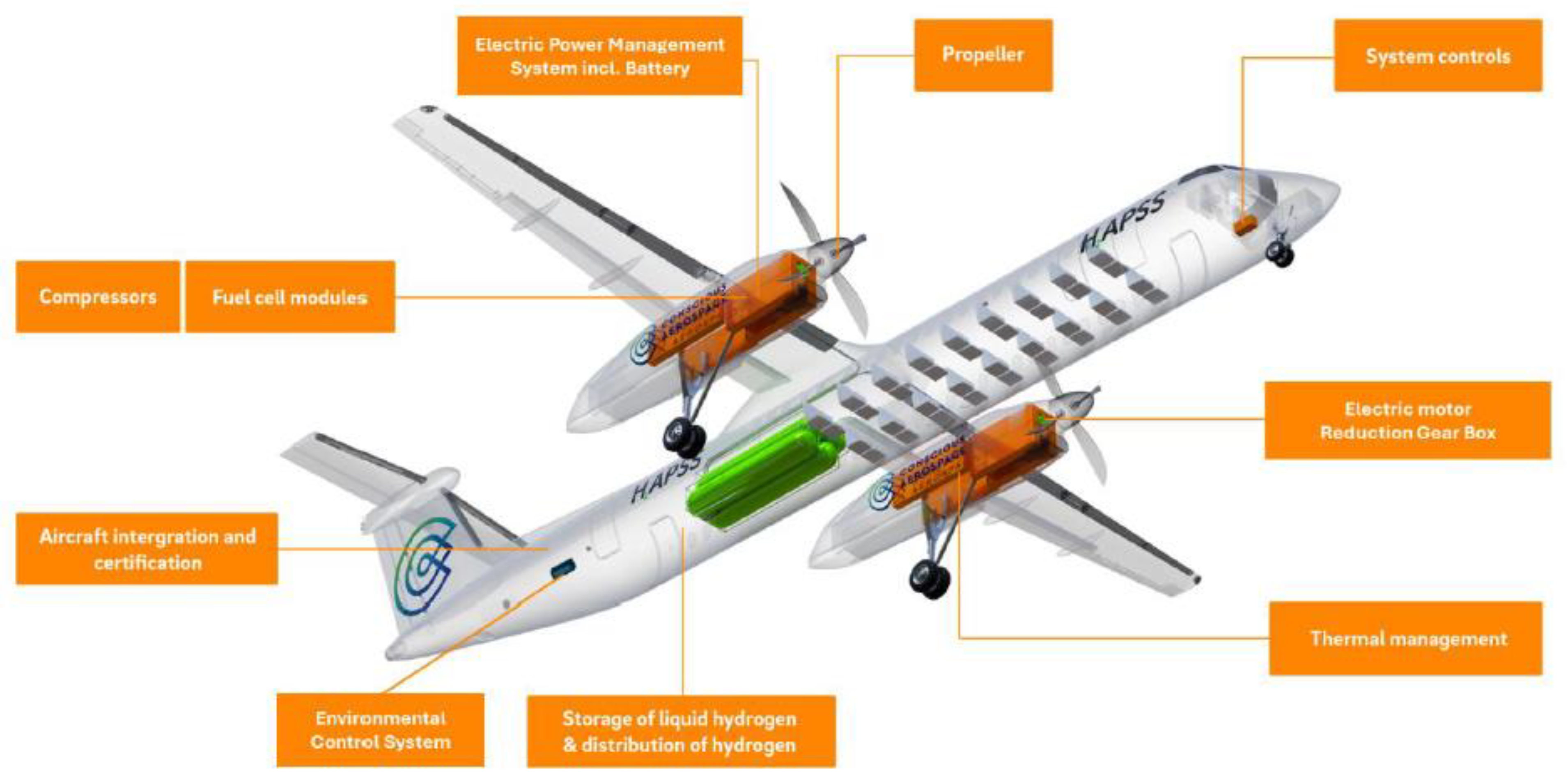
Figure 2.
Air New Zealand Dash 8-300 (2017), copyright picture by Jordan Tan, via Shutterstock (StockFoto ID: 729358585).
Figure 2.
Air New Zealand Dash 8-300 (2017), copyright picture by Jordan Tan, via Shutterstock (StockFoto ID: 729358585).
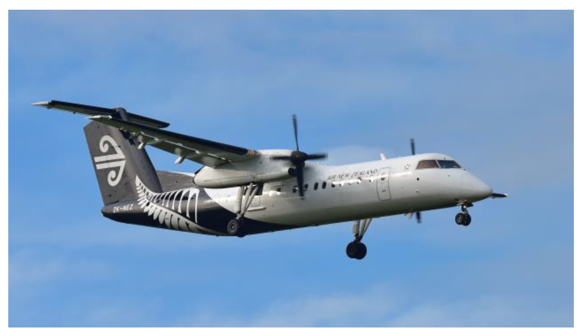
Figure 3.
Performance simulation model scheme.
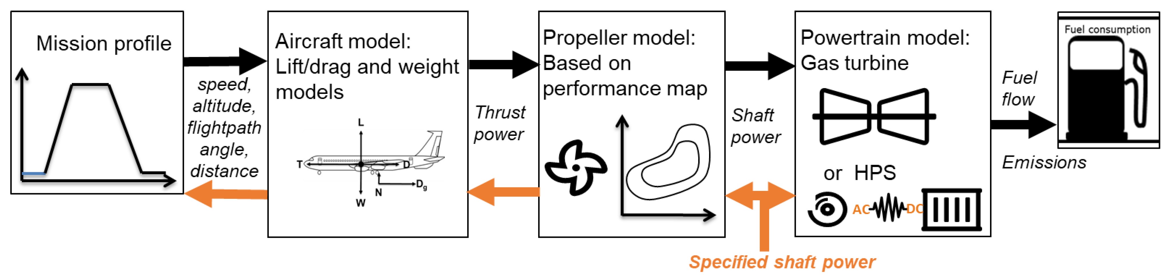
Figure 4.
Example mission profile information for the Dash 8-300, adapted from Ref. [22].
Figure 4.
Example mission profile information for the Dash 8-300, adapted from Ref. [22].
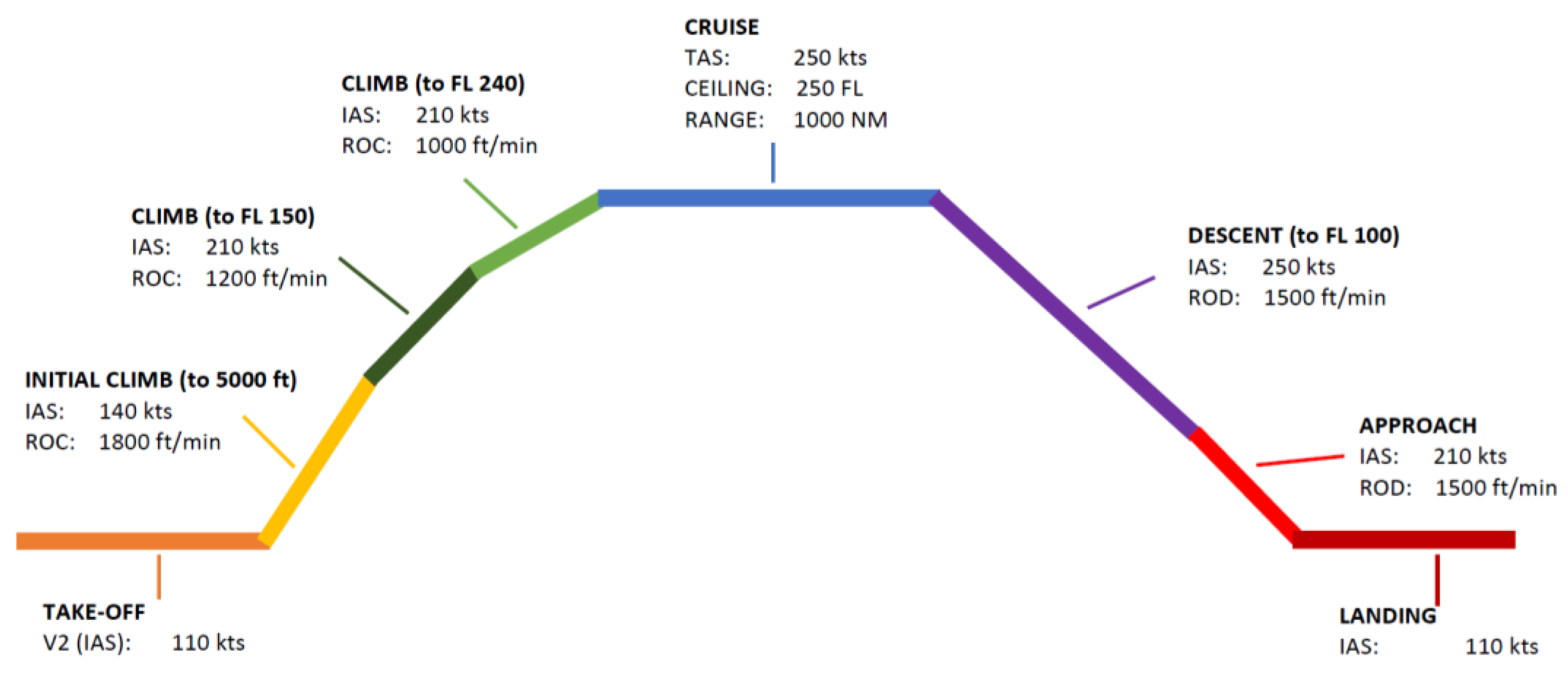
Figure 5.
Division of the takeoff phase into segments determined by flap, landing gear and power settings.
Figure 5.
Division of the takeoff phase into segments determined by flap, landing gear and power settings.
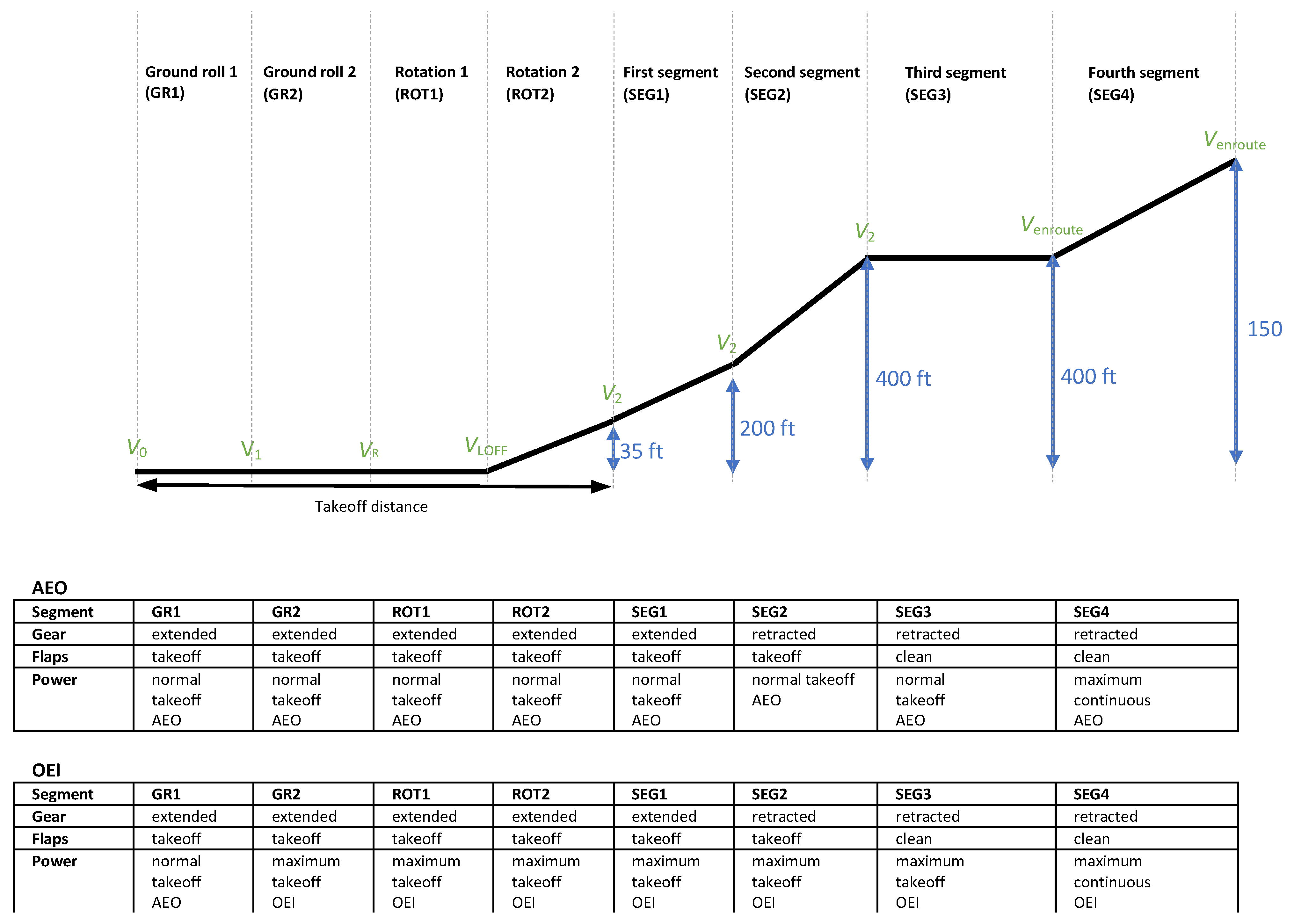
Figure 6.
Illustration 2 of the forces in the basic aerodynamic “point mass” model, with forces: D drag, Dg ground friction, N normal, L lift, W weight and T thrust.
Figure 6.
Illustration 2 of the forces in the basic aerodynamic “point mass” model, with forces: D drag, Dg ground friction, N normal, L lift, W weight and T thrust.
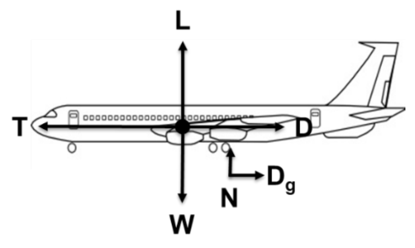
Figure 7.
Comparison of drag polars (clean configuration) by lift-to-drag ratio L/D as function of lift coefficient .
Figure 7.
Comparison of drag polars (clean configuration) by lift-to-drag ratio L/D as function of lift coefficient .
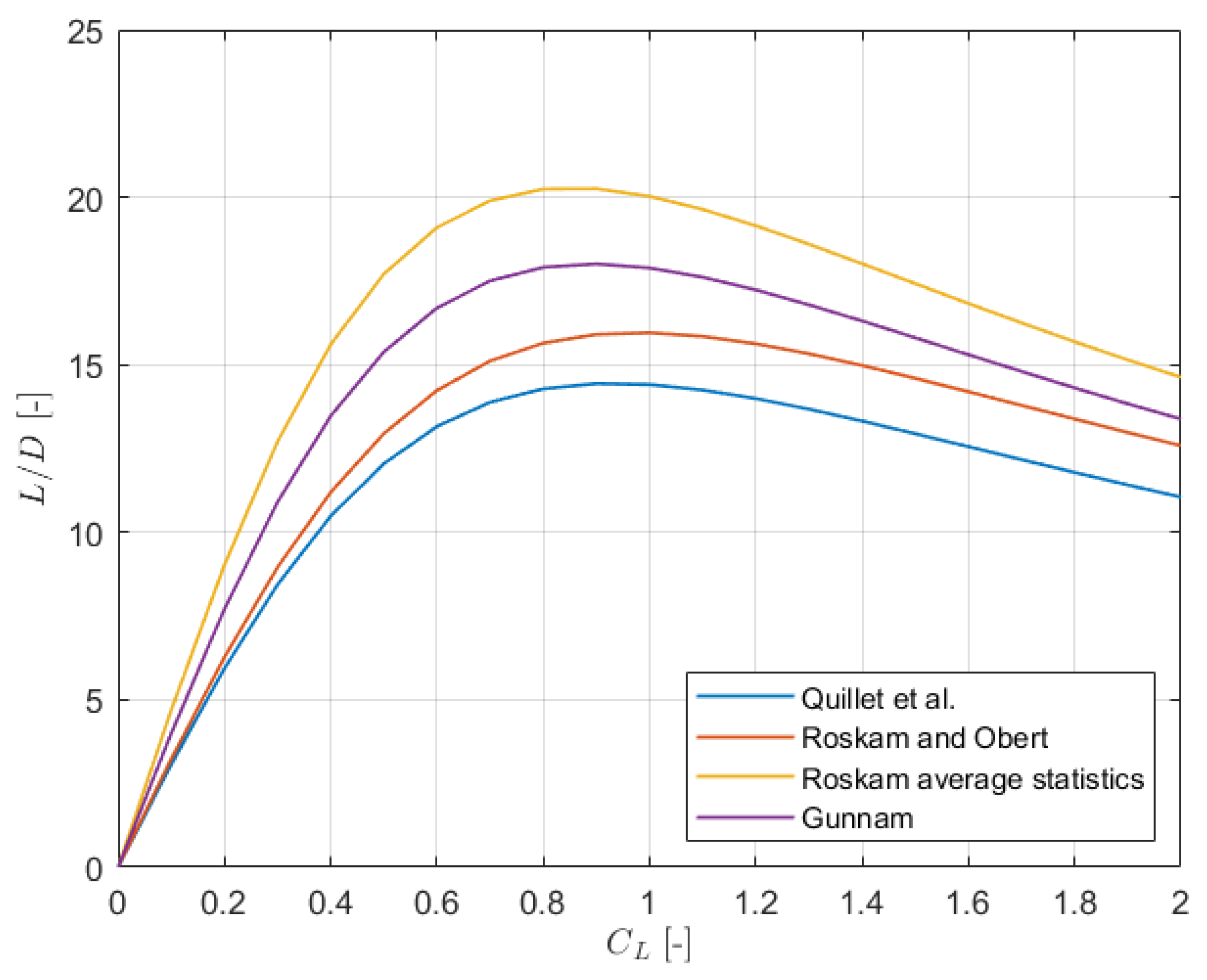
Figure 8.
Depiction of the Dash 8-300 propeller map , reproduced from Ref. [26].
Figure 8.
Depiction of the Dash 8-300 propeller map , reproduced from Ref. [26].
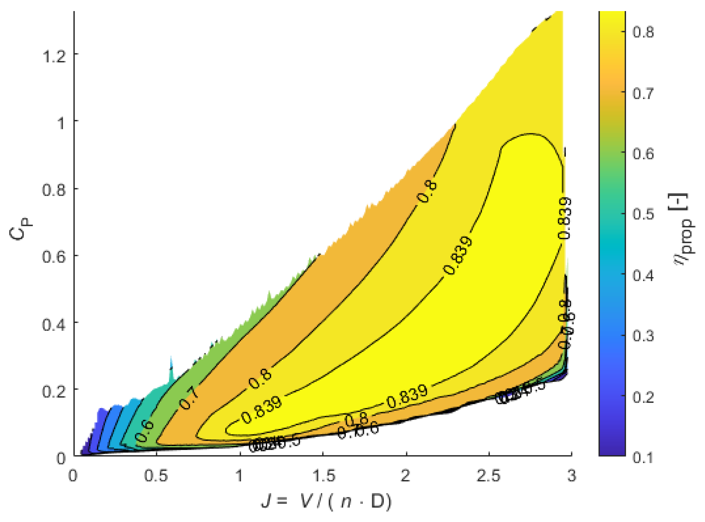
Figure 9.
Depiction of the Dash 8-300 propeller map
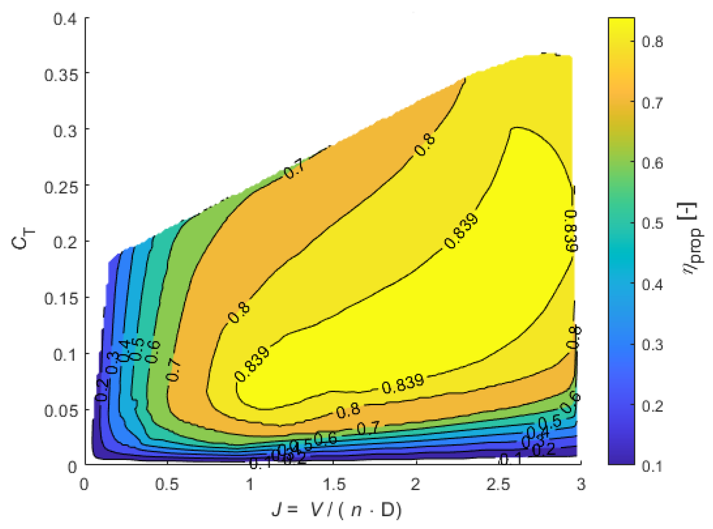
Figure 10.
Illustrating scheme of HPS architecture, with four FCS modules.
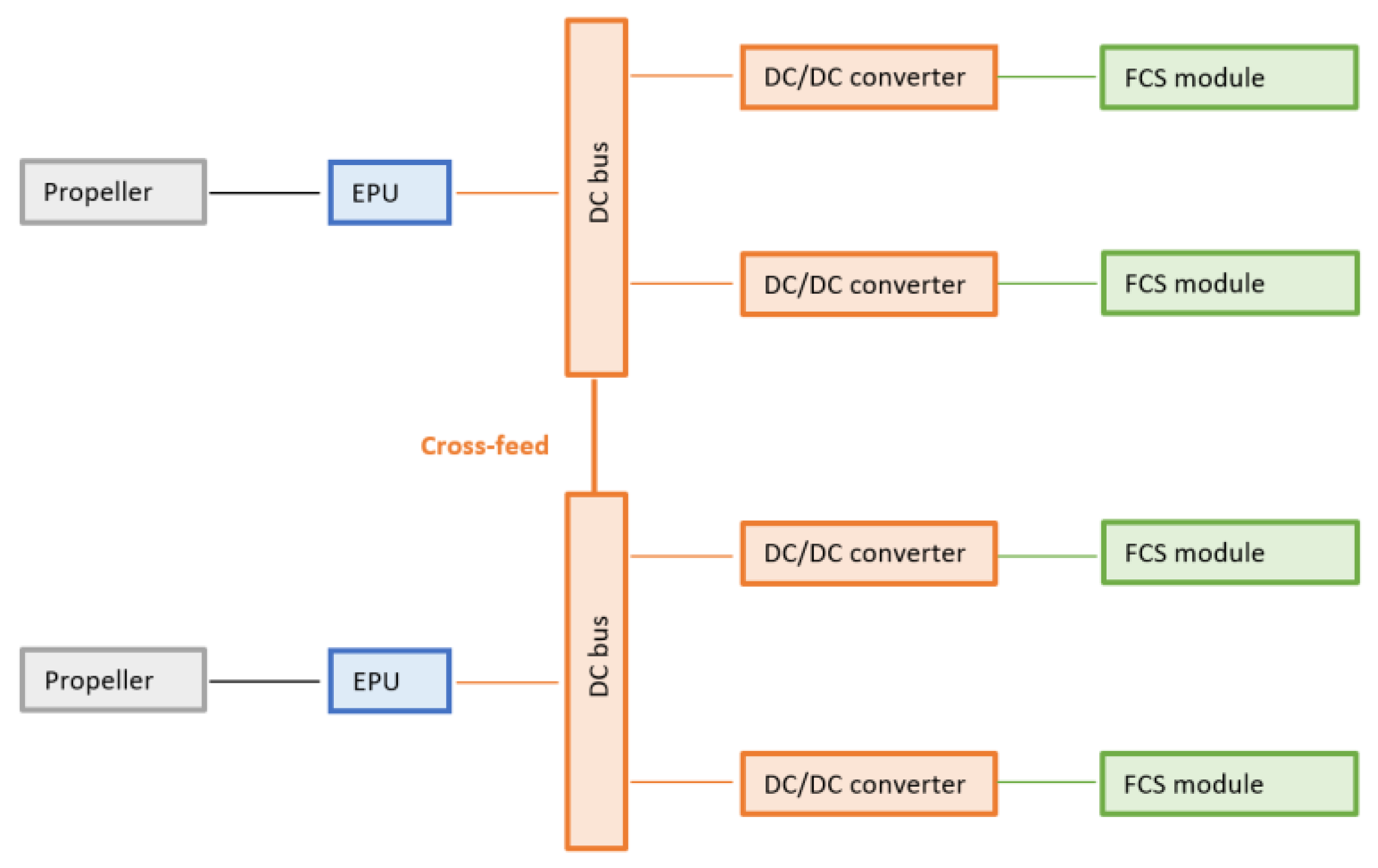
Figure 11.
Illustrating scheme of the FCS model.
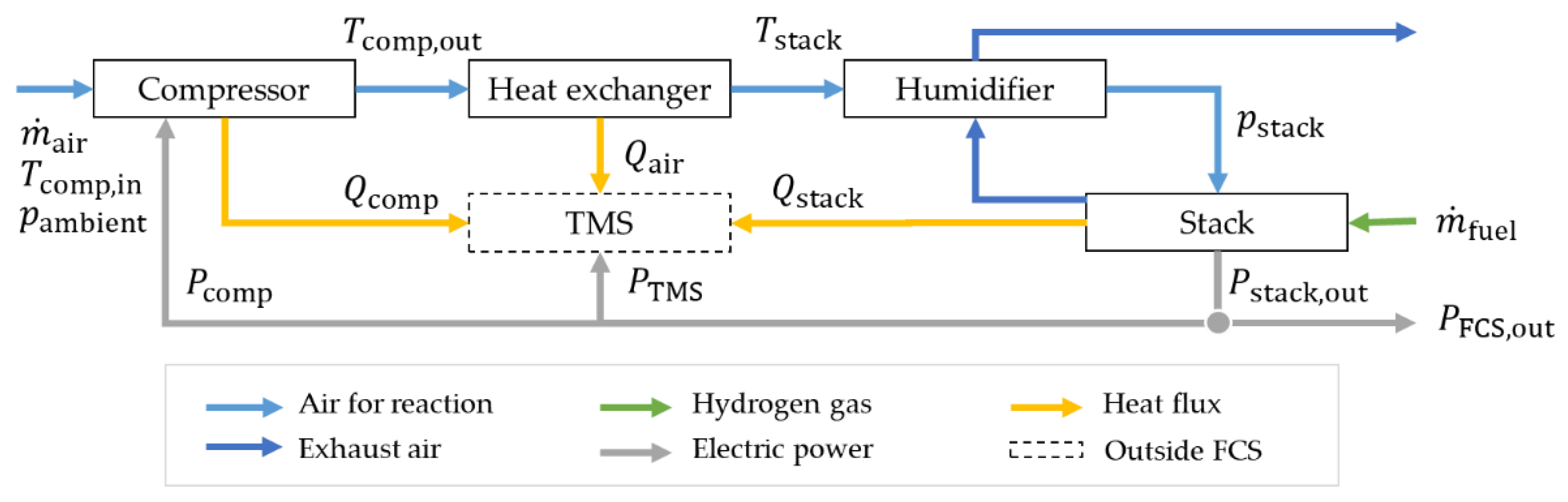
Figure 12.
Map relating FC stack pressure and power density to cell voltage, derived from Ref. [34].
Figure 12.
Map relating FC stack pressure and power density to cell voltage, derived from Ref. [34].
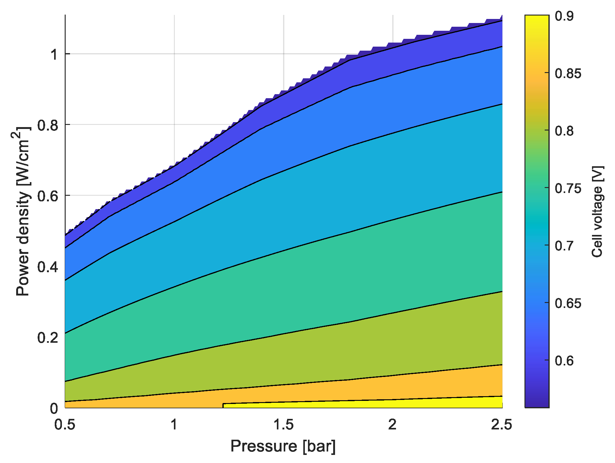
Figure 13.
Relation between FC stack pressure and temperature in the ElringKlinger stack, derived from Ref. [34].
Figure 13.
Relation between FC stack pressure and temperature in the ElringKlinger stack, derived from Ref. [34].
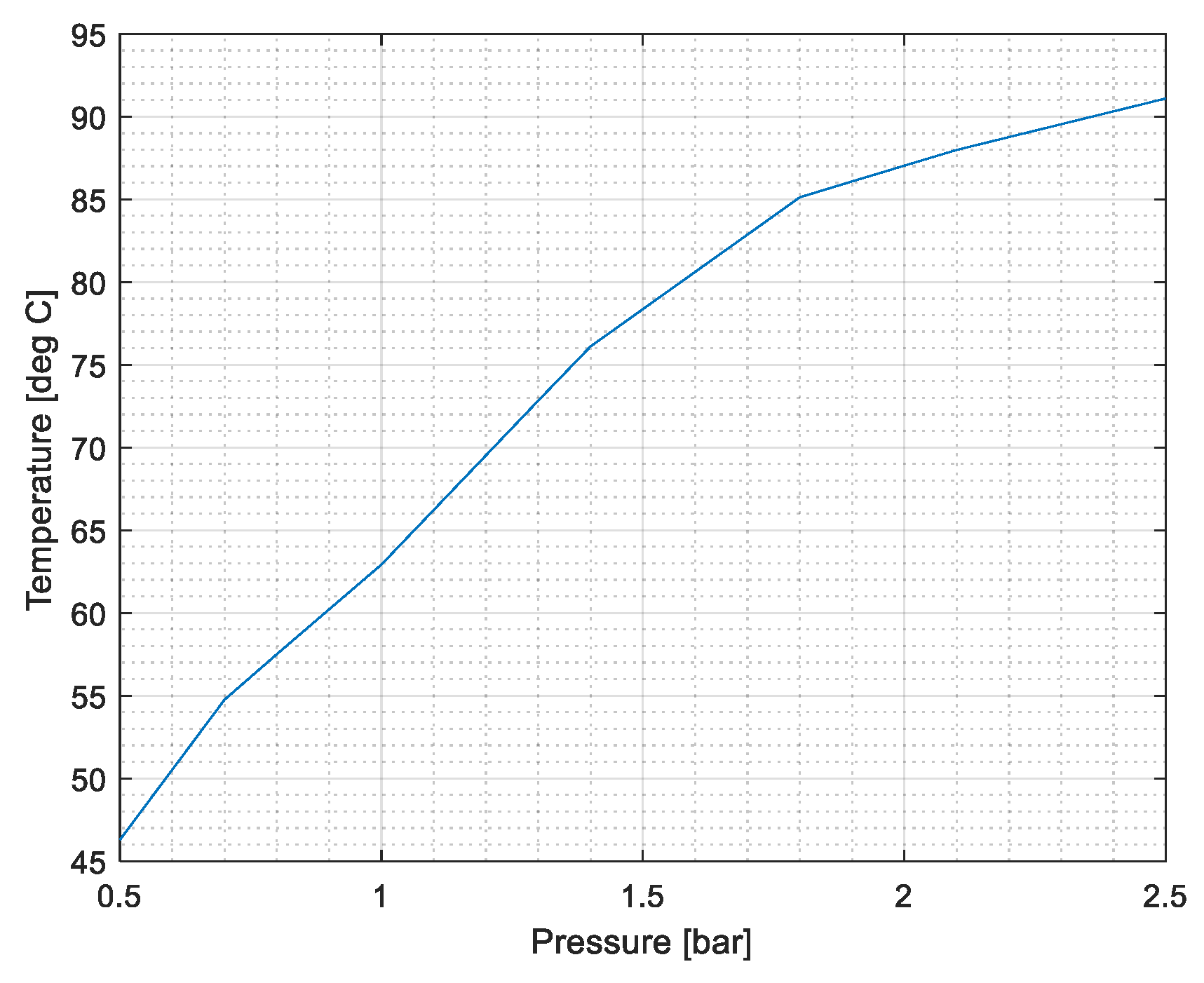
Figure 14.
Derived FCS efficiency model, as function of altitude and output power demand. In red, the altitude-dependent maximum system power limit from Ref. [34] is indicated.
Figure 14.
Derived FCS efficiency model, as function of altitude and output power demand. In red, the altitude-dependent maximum system power limit from Ref. [34] is indicated.
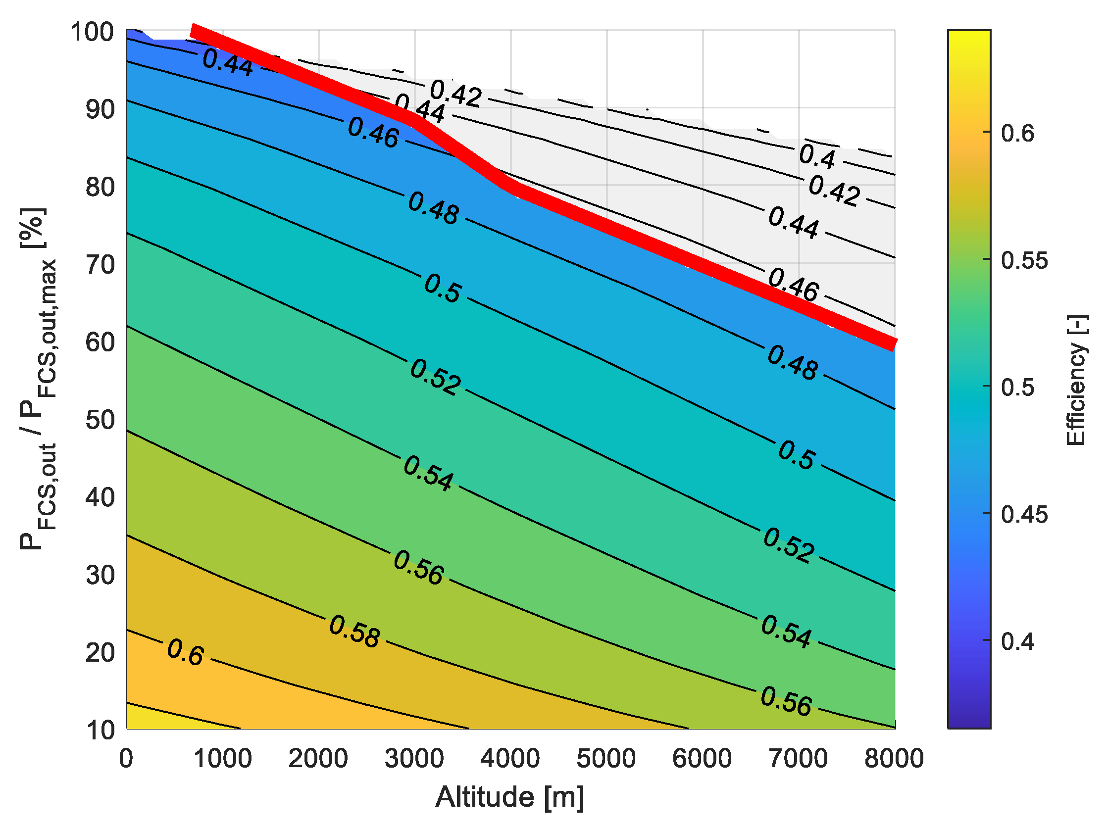
Figure 15.
TOD segment simulation results with the reference aircraft.
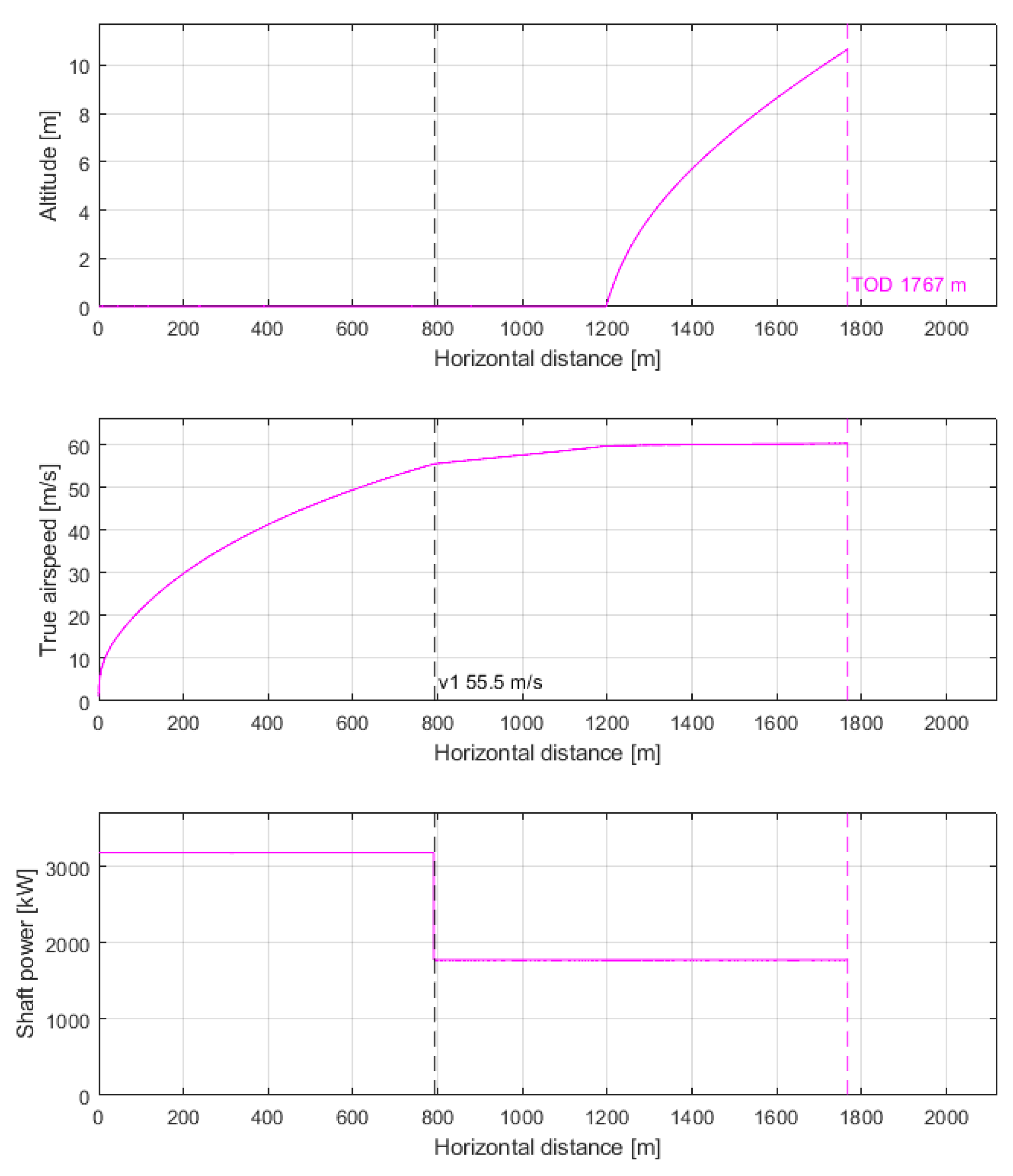
Figure 16.
Comparison of simulated and reference takeoff distances [17] at ISA sea level conditions.
Figure 16.
Comparison of simulated and reference takeoff distances [17] at ISA sea level conditions.
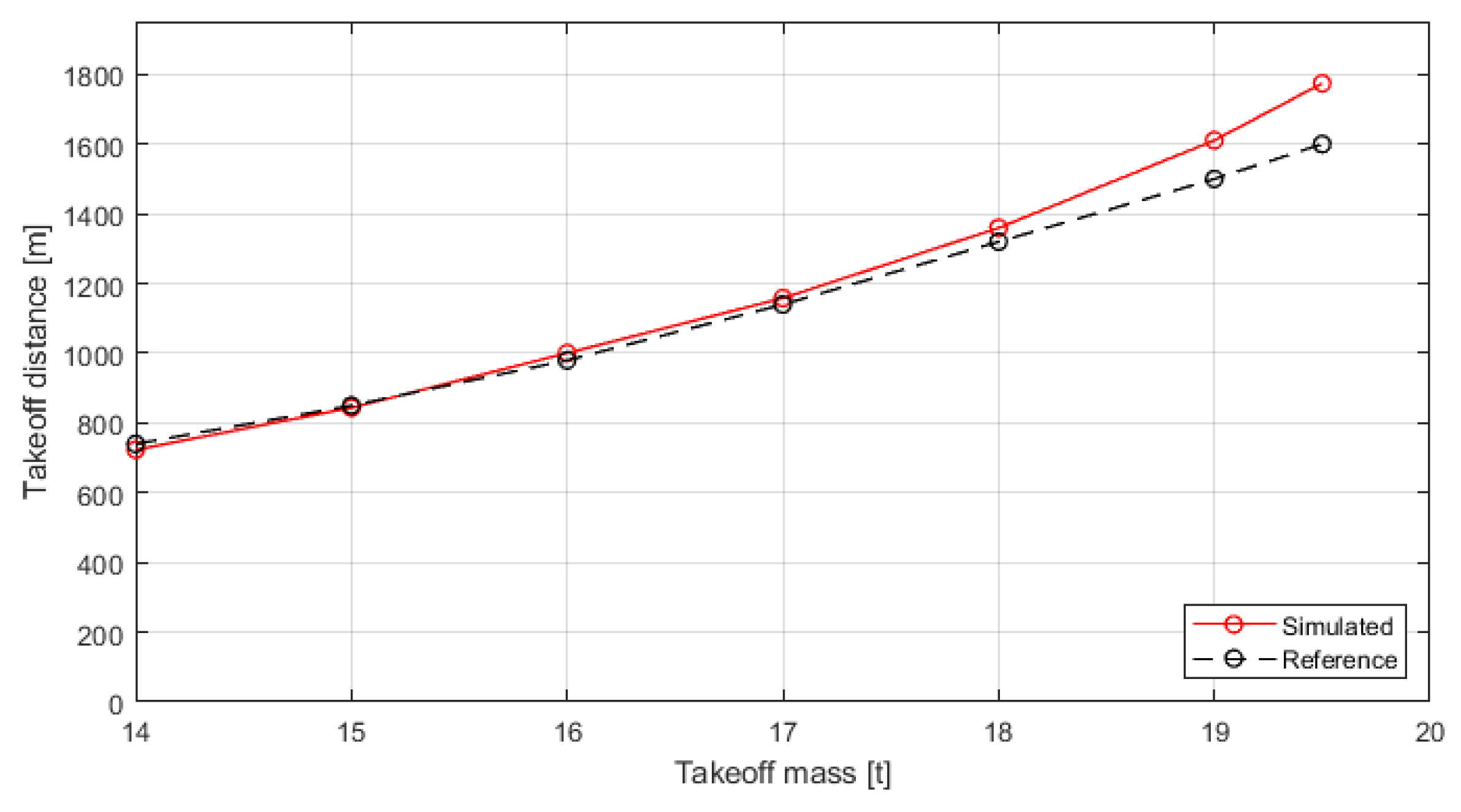
Figure 17.
Takeoff simulation results with the HAPSS aircraft model for the OEI case.
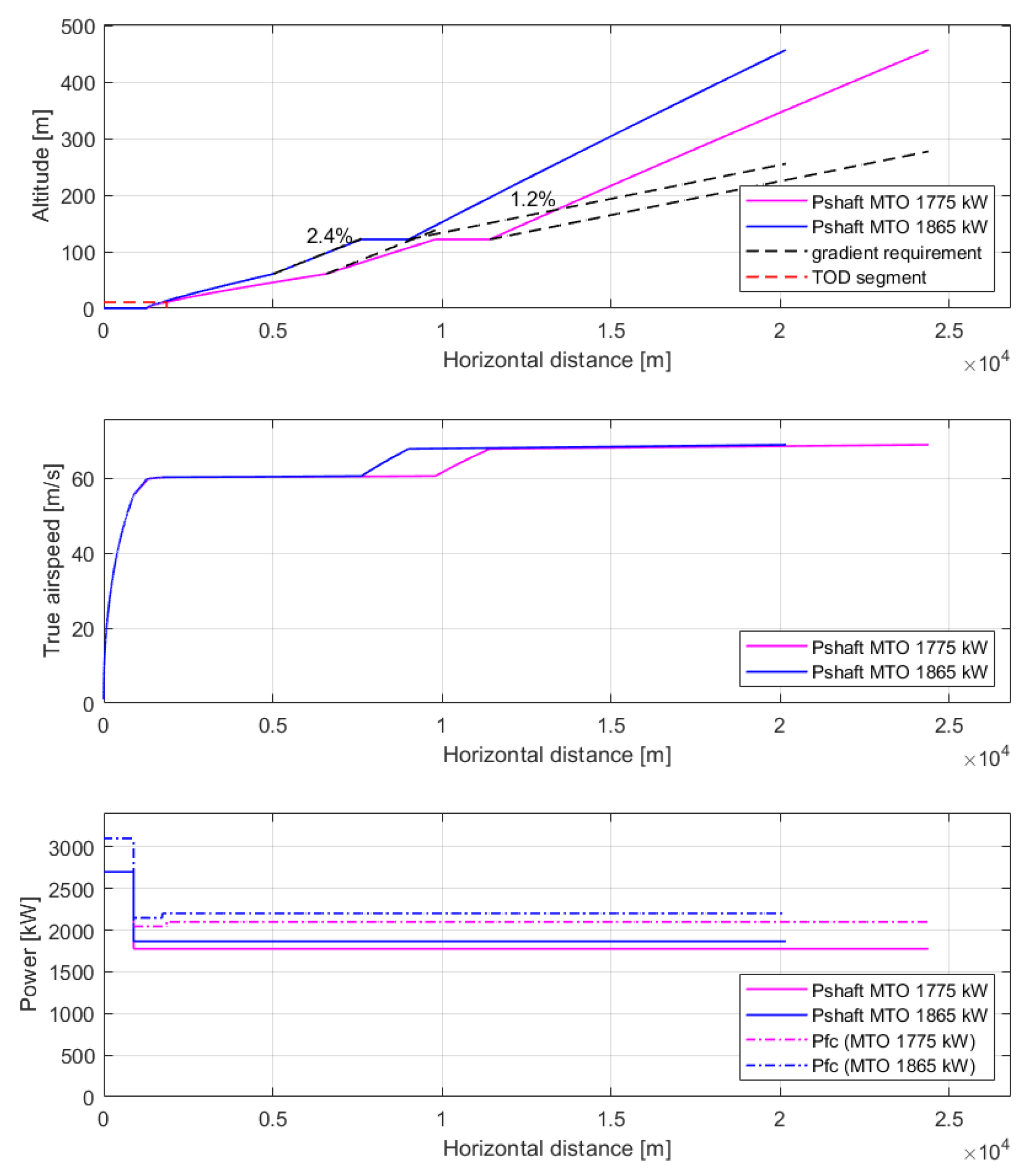
Figure 18.
Takeoff distance segment simulation results with the HAPSS aircraft model for the OEI case.
Figure 18.
Takeoff distance segment simulation results with the HAPSS aircraft model for the OEI case.
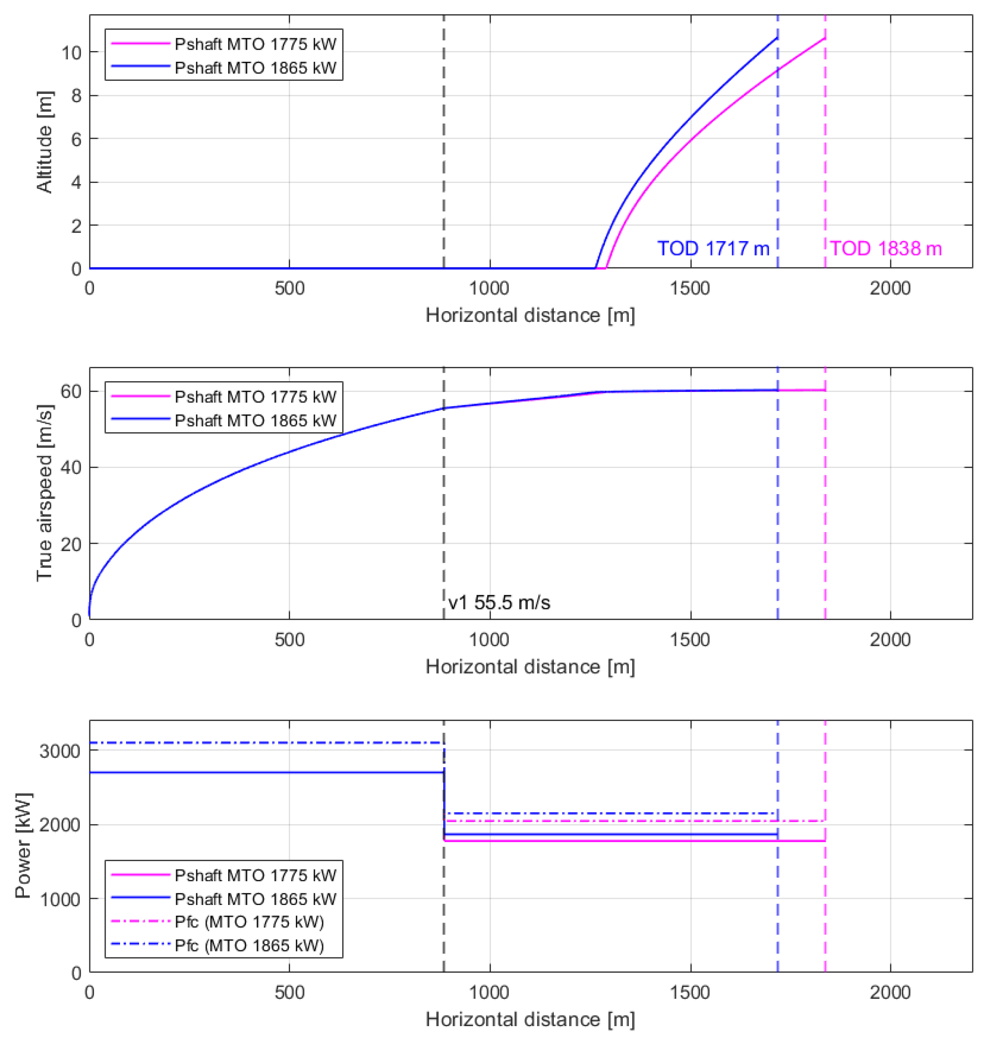
Figure 19.
Sensitivity results for the takeoff distance (left) and second segment gradient (right) for various model parameters (expressed as percental deviation from the reference value).
Figure 19.
Sensitivity results for the takeoff distance (left) and second segment gradient (right) for various model parameters (expressed as percental deviation from the reference value).
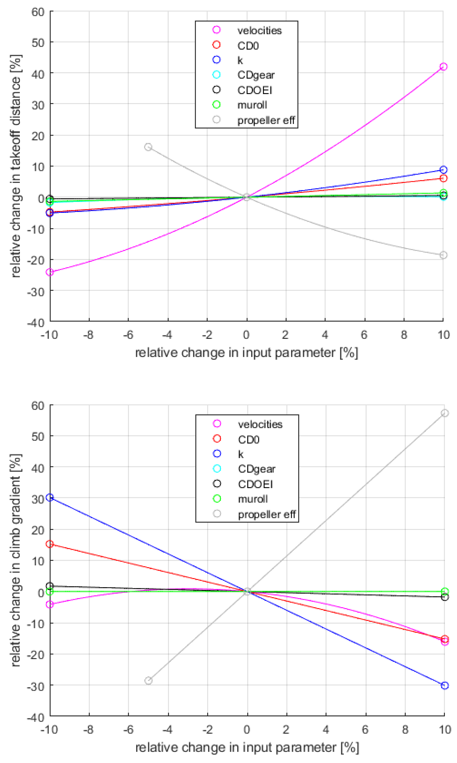
Figure 20.
Fuel cell heat production for different speeds at which the NTO shaft power is reached.
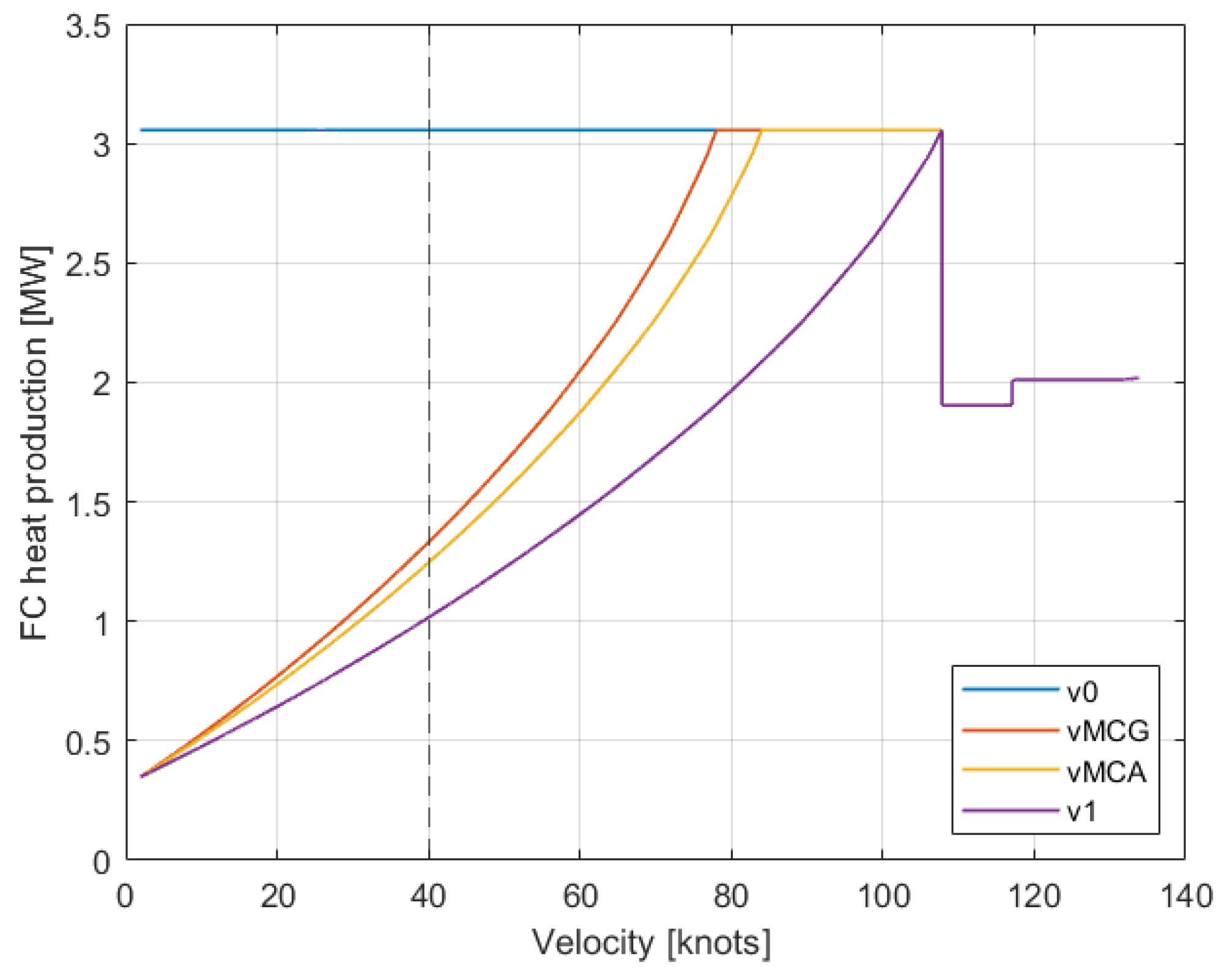
Figure 21.
Go-around simulation results with the HAPSS aircraft model (OEI case) illustrating the gradient requirement.
Figure 21.
Go-around simulation results with the HAPSS aircraft model (OEI case) illustrating the gradient requirement.
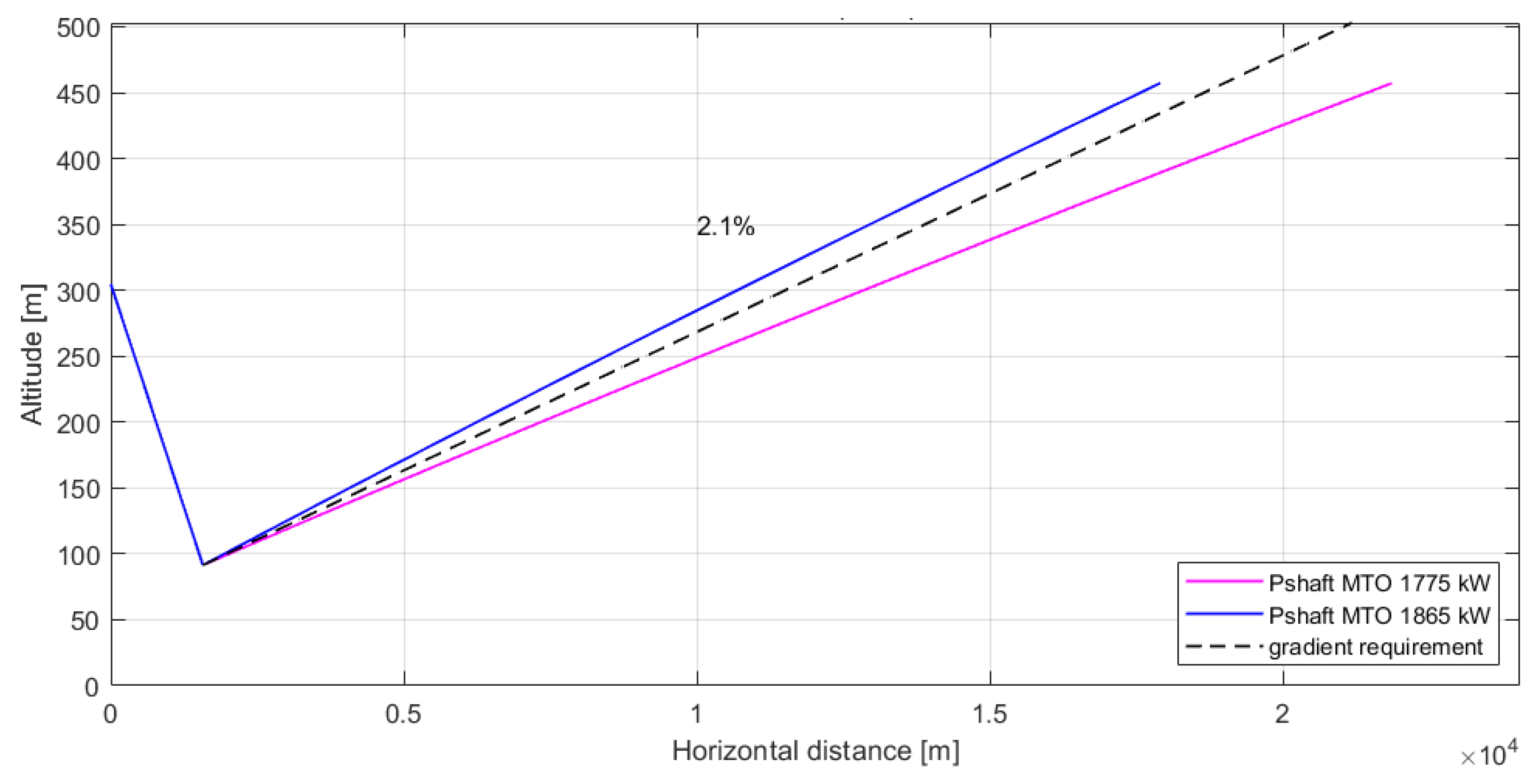
Figure 22.
Climb performance plots for various FCS rated powers, compared with reference aircraft data.
Figure 22.
Climb performance plots for various FCS rated powers, compared with reference aircraft data.
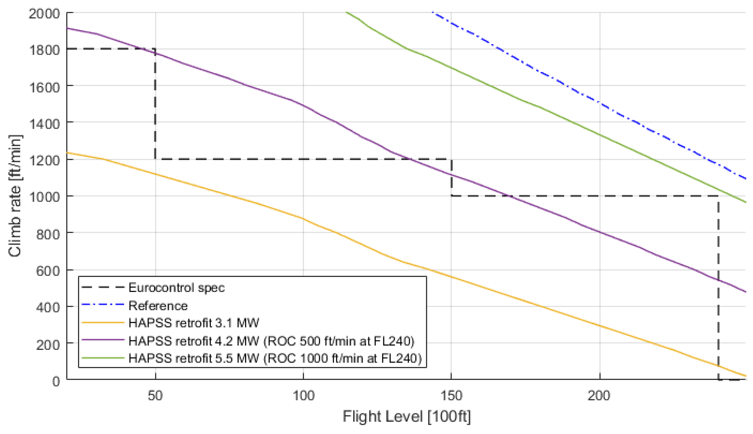
Figure 23.
RSEC for various cruise altitudes and speed conditions, for the reference kerosene aircraft (left) and the HAPSS aircraft (right).
Figure 23.
RSEC for various cruise altitudes and speed conditions, for the reference kerosene aircraft (left) and the HAPSS aircraft (right).
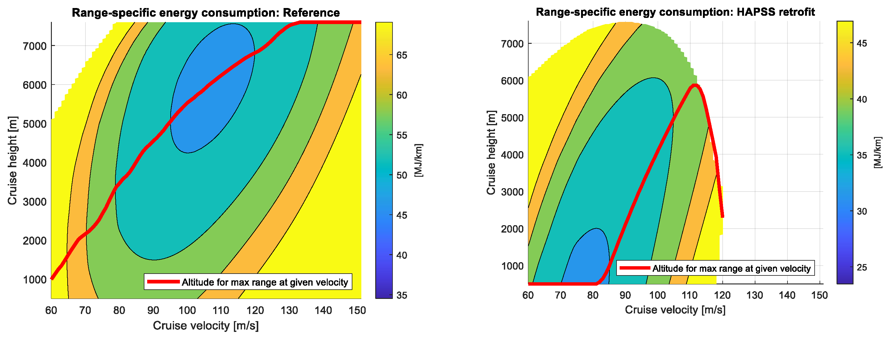

Table 1.
Applied reference aircraft data.
| Parameter | Description | Value [17,18,19,20] |
|---|---|---|
| Aircraft | Aircraft model | 311 |
| R | Range | 920 NM (1704 km) |
| hCr | Maximum cruise altitude | 25000 ft (7620 m) |
| vCr | Cruise true air speed | 133 m/s (480 km/h) |
| MTOM | Maximum takeoff mass | 19505 kg |
| MLM | Maximum landing mass | 19051 kg |
| DPM | Design payload mass | 5300 kg |
| OEM | Operational empty mass | 11653 kg |
| Sw | Wing area | 56.3 m2 |
| Bw | Wing span | 27.4 m |
| Np | Number of engines / propellers | 2 |
| Engine | Engine type | Pratt & Whitney PW123 |
| MTO power | Maximum takeoff (shaft) power, per engine |
1775 kW |
| Propeller | Propeller type | Hamilton Sundstrand 14SF |
| Dp | Propeller diameter | 3.96 m |
| Bp | Number of propeller blades | 4 |
Table 2.
Summary of compared drag polar coefficients (clean configuration).
| Source | [-] | Lift-Induced Drag Coefficient k [-] |
|---|---|---|
| Gunnam [25] | 0.0247 | 0.0312 |
| Quillet et al [26] | 0.0322 | 0.0372 |
| Roskam averaged Statistics [27] |
0.0210 | 0.0289 |
| Roskam & Obert [28] | 0.0306 | 0.0320 |
Table 3.
Clean and takeoff drag polar coefficients applied.
| Aircraft Configuration | [-] | Lift-induced drag coefficient k [-] |
|---|---|---|
| Clean | 0.0322 | 0.0372 |
| Takeoff flaps | 0.0422 | 0.0403 |
| Takeoff flaps + Landing gear |
0.0572 | 0.0403 |
Table 4.
Modelled fuel flow and PSFC values for typical mission operating points.
| Mission Phase | h [m] | v [m/s] |
(1 Engine) [kW] | (1 Engine) [kg/h] | [kg/kWh] |
|---|---|---|---|---|---|
| taxi | 0 | 10 | 100 | 86 | 0.860 |
| take off | 0 | 0 | 1775 | 507 | 0.285 |
| climb | 4000 | 100 | 1603 | 462 | 0.288 |
| cruise | 7620 | 133 | 1062 | 301 | 0.284 |
| descent | 4000 | 100 | 100 | 62 | 0.615 |
| landing | 0 | 0 | 855 | 267 | 0.321 |
Table 5.
FCS model parameters.
| Parameter | Symbol | Value |
|---|---|---|
| Air filter pressure drop [34] | - | 5e2 Pa |
| Humidifier pressure drop (supply side) [34] | - | 5e3 Pa |
| Heat exchanger pressure drop (supply side) [34] | - | 1e4 Pa |
| Specific heat capacity (for air) | 1006 J/kg/K | |
| Ratio of the specific heat capacities (for air) | 1.4 | |
| Compressor isentropic efficiency [36] | 0.76 | |
| Compressor driver efficiency (mechanical, electrical and power conversion efficiency) [36] | 0.97 0.94 0.95 = 0.87 |
Table 6.
Speed at which max takeoff power is reached with corresponding impact on TOD and cooling demand.
Table 6.
Speed at which max takeoff power is reached with corresponding impact on TOD and cooling demand.
| Speed Cases (at Which Max Power Is Reached) | Speed Value [kts] |
TOD [m], Determined by OEI Condition | Cooling Demand [MW] (at v = 40 kts) |
|---|---|---|---|
| from the start (reference case v0) | 0 | 1717 | 3.06 |
| ground minimum control speed vMCG | 78 | 1869 | 1.33 |
| air minimum control speed vMCA | 84 | 1901 | 1.25 |
| decision speed v1 | 108 | 2071 | 1.02 |
Disclaimer/Publisher’s Note: The statements, opinions and data contained in all publications are solely those of the individual author(s) and contributor(s) and not of MDPI and/or the editor(s). MDPI and/or the editor(s) disclaim responsibility for any injury to people or property resulting from any ideas, methods, instructions or products referred to in the content. |
© 2024 by the authors. Licensee MDPI, Basel, Switzerland. This article is an open access article distributed under the terms and conditions of the Creative Commons Attribution (CC BY) license (http://creativecommons.org/licenses/by/4.0/).
Copyright: This open access article is published under a Creative Commons CC BY 4.0 license, which permit the free download, distribution, and reuse, provided that the author and preprint are cited in any reuse.


