Submitted:
05 December 2024
Posted:
06 December 2024
Read the latest preprint version here
Abstract
Since for finite systems the thermodynamic potentials are not equivalent the fluctuation induced forces defined in any of them lead to different forces - Casimir force (CF) in grand canonical ensemble (GCE) and Helmholtz force (HF) in canonical (CE) one with fixed magnetization. Here we consider the HF within Nagle-Kardar model with periodic boundary conditions. Thus, the current study is complimentary to the recent one for the CF, see , in the same model. We remind that the model represents one-dimensional Ising chain with long-range equivalent-neighbor ferromagnetic interactions of strength Jl/N>0 superimposed on the nearest-neighbor interactions of strength Js which could be either ferromagnetic (Js>0) or antiferromagnetic (Js<0). In the infinite system limit the model exhibits in the plane (Ks=βJs,Kl=βJl) a critical line 2Kl=exp−2Ks,Ks>−ln(3)/4, which ends at a tricritical point (Kl=−3/2,Ks=−ln(3)/4). The obtained results demonstrate that the temperature behavior of the HF differs essentially form the one of the CF. Furthermore, we show that the CE and GCE are not equivalent for the current model - even in the thermodynamic limit. Finally, in the phase space {Ks,Kl,m} we determine the regions of stable states of the system.
Keywords:
finite-size effects
; exact results
; Helmholtz force
; Casimir force
; Nagle-Kardar model
; phase transitions
; critical phenomena
; phase diagrams
1. Introduction
In any physical systems there are fluctuations. If the temperature T is low, this is due to the quantum nature of its constituents. When T increases, temperature fluctuations set in and become dominant. If the fluctuations are mediated by massless excitations that can freely proliferate, they lead to long ranged interactions, called fluctuation induced forces, between any two bodies immersed in such a medium. The currently most prominent example of a fluctuation-induced force is the one due to quantum or thermal fluctuations of the electromagnetic field, leading to the so-called QED Casimir effect, named after the Dutch physicist H.B. Casimir. In 1948 he first realized that in the case of two perfectly-conducting, uncharged, and smooth plates parallel to each other in vacuum at , these fluctuations lead to an attractive force between them [2]. Thirty years after Casimir’s publication, Fisher and De Gennes [3] showed that a very similar effect exists in critical fluids, today known as the critical Casimir effect. Depending on the boundary conditions imposed on the surfaces bounding the system, the Casimir force can be bot attractive and repulsive. A summary of the results available for this effect can be found in the recent reviews [4,5,6,7]. Naturally, the effect takes place only in finite systems. Thus, the description of the critical Casimir effect is based on finite-size scaling theory [8,9,10]. The effect is more than a theoretical construction within statistical mechanics—the critical Casimir effect has been observed experimentally [11,12,13,14,15] in a variety of systems.
Within equilibrium statistical mechanics, thermodynamic ensembles are described in terms of specific thermodynamic potentials, through which thermodynamic parameters control the macroscopic behavior of considered systems. One can define a fluctuation induced force in any of them. This can be motivated by the physical situation. The ensembles are, normally, thermodynamically equivalent in the bulk limit. The fluctuation induced forces are defined, however, in a system with at least one finite dimension, i.e., within finite systems. Thus, the forces defined in two different ensembles for any given model shall be expected to be, in principal, with a different behavior - at least as a function of the characteristic finite size L and the temperature T. Recently this has been demonstrated explicitly in the example of the fluctuation induced force in a system with fixed value of the total magnetization [16,17,18,19]. The corresponding fluctuation induced force has been defined in [16] in the case of an Ising chain and called Helmholtz force. In [16,17,18,19] it has been shown that the behavior of the Helmholtz force is quite different from that of the Casimir force. This has been done for periodic, antiperiodic, Dirichlet boundary condition, as well as for the Ising chain with a defect bond. In the current article we continue the study of the ensemble dependence of the fluctuation induced forces in the example of the Nagle-Kardar model. More specifically, we consider the Helmholtz force in a model Hamiltonian [20,21,22] with two competing interactions: the Ising model on a chain with “ nearest-neighbor" and with “infinitesimal equivalent-neighbor" interactions between the spins. This is also known as the Nagle-Kardar model (for reviews see [23,24,25]). The Hamiltonian of the model is:
where the following notations: , are used. Given the symmetry of the problem it suffices to fix magnetization .
The first term on the right hand side of (1) describes the Ising model with short-ranged interactions between nearest neighbors on a spin chain with periodic boundary conditions and with with interaction constant . The second term is the equivalent-neighbor Ising model with infinitesimal long-ranged interaction between spins characterized by . With one obtains the so-called Husimi-Temperley model [26,27]. In the case considered here, the nearest-neighbor interaction is either ferromagnetic or antiferromagnetic, i.e., or , while the long-range interaction is always ferromagnetic, i.e., . It can be shown that when there is no long-range order in the bulk system at any finite temperature.
Initially, this model was introduced within the grand canonical ensemble, in the presence of an external field h, by Baker in 1969 [20]. Actually, subsequent considerations of the model have been mainly carried out in the grand canonical ensemble. The seminal contributions of Nagle [21] and Kardar [22] demonstrated that the model is instructive as a means to analyze complicated phase diagrams and crossover phenomena arising from the competition between ferromagnetic and antiferromagnetic interactions. A wide range of physical and mathematical problems have been revealed by this simple long-range interaction reviving interest in one-dimensional Ising systems [23,24,25,28,29,30,31,32,33,34,35,36,37,38,39,40,41], which has proven to be a fertile platform for the investigation of various generalizations of the competition between the antiferromagnetic and ferromagnetic interactions [39,40,42,43,44,45,46,47,48,49]. In particular it has been shown that this simple system may well describe a number of interesting phenomena, including ensemble inequivalence [34,36,49], negative specific heat[34,35,36], ergodicity breaking [34,35,36], long-lived thermodynamically unstable states [34,35], the prospect of analysis of different information estimators [42] and the cooling process of a long-range system [50]. The bulk thermodynamic properties of the model have been actively studied in both the grand canonical [21,22,30,51] and the microcanonical ensemble [25,34,35,36,47].
We are not aware of the behavior of the Nagle-Kardar model within the canonical ensemble (with fixed magnetization) having been reported in any research up to this time—even in the case of the bulk limit. Here we will discuss it in a finite chain in that ensemble subject to periodic boundary conditions.
We note that there are systems for which the statistical-mechanical ensembles are not equivalent, even in the thermodynamic limit. One example is the case of systems with non-additive interactions [52,53]. The second term in Eq. (1) is an example of such an interaction. As we will see, it leads to as non-convex behavior of the Helmholtz free energy in the canonical ensemble. In this case there are stable, metastable and unstable states in the system. For the Nagle-Kardar model we will determine their position in the plane.
We have derived the behavior of this system not only in the thermodynamic limit, in which its phase diagram is highly non-trivial—see below—but also when the system is finite, in which case the fluctuation-induced critical Helmholtz force (HF) can be defined and studied.
The structure of the article is as follows. We define the model in Section 2. In Section 3 we determine the phase diagram of the model. Then, Section 4 contains our analysis of the stable, metastable and unstable states of the system and the determination of their positions. The behavior of the Helmholtz force is elucidated in Section 5. The article ends with a conclusion and discussion section, in Section 6.
2. The Model in Canonical Ensemble
We start with the calculation of the canonical partition function
where
Obviously
Knowing the partition function for the short-range Ising model under periodic boundary conditions with fixed magnetization [16], which equals the sum that remains in Eq. (4), it is easy to determine the partition function :
where 2 is the generalized hypergeometric function [54]. From Eq. (5) it immediately follows that the Helmholtz free energy density of the model takes the form:
with the Helmholtz free energy density of the one-dimensional Ising model:
Let minimize the Helmholtz free energy given by Eq.(8), i.e. . Then this, from now on to be referred to as the equilibrium magnetization , is given by the solution of the equation
Explicitly, one has
For any fixed values of and the free energy attains an extremum as a function of m, in that it is a minimum, at when the system is in unordered phase; in the ordered phase this equation has more than one solution. In that case, at the free energy usually attains a maximum there and possesses two minima at . As we will see below, the system considered here also exhibits a tricritical point. There, the free energy, Eq. (8), shows three equally deep minima, one of which is at .
We note that corresponds to the analogous solution for magnetization of the same model in the grand canonical ensembles with —see Eq. (7) in [1]; there the actual magnetization of the system indeed is .
3. On the Phase Diagram in Canonical Ensemble
We start by briefly commenting on how one can determine the phase diagram in the model.
Expanding , see Eq. (8), about we obtain
Keeping in mind that when the and terms vanish as function of their parameters determes the critical, i.e., the second order phase transition line, and tricritical behavior of the system, respectively, we find
- the second order phase transition exists when , with ;
- there is a tricritical point in the system at , i.e., .
4. On the Stability of the System
In the current section we will study the region of the stability of the states of Nagle-Kardar model within the canonical ensemble. Let us remind that in the current model any state is characterized by coordinates.
According to thermodynamics
and
Obviously, the system will be stable if
The last inequality implies that, when it is valid, the free energy is a convex function of .
From Eq. (8) it follows that the above condition is equivalent to
Obviously, the last can be rewritten as
The second inequality, concerning the Ising model, is fulfilled for all values of and m. The first, however, is not. For any nonzero finite value of it will be a region, for which the system will be unstable. Explicitly, one has
The above expression determines the equation of the "spinodal surface" of the magnetization , called "spinodal magnetization", as a function of and
Obviously, the spinodal surface indicates onset of metastability. Let us note that the susceptibility in the grand canonical ensemble, since it represents there the mathematical dispersion of the sum of spins, is always positive. Thus, in the regions, where Eq. (17) is violated, CE and GCE for the Nagle-Kardar model are not equivalent, even in the thermodynamic limit.
For a few limiting cases one can easily obtain explicit solutions for . For example, setting in Eq. (20) , we obtain the well-know result [52] for the Husimi-Temperley model [26,27]
For the solution of Eq. (20) can also be directly found. It is
One can also immediately show that when , formally the same solution of the above equation for , up to the leading order, is also valid (but for other restrictions over and ).
The regions of stability in the system are visualized in Figure 1 for . Figure 2, left, visualizes the spinodal surface and the region below it, for which the system is with positive second derivative of the free energy with respect to m which embraces the regions of thermodynamically stability. Above this region everywhere where <0 the system is thermodynamically unstable for the corresponding . The right panel shows the cross sections of this region with planes at given values of , for and . Figure 3 shows the behavior of the bulk free energy as a function of m for the regions where system is stable, with free energy being convex, metastable - with a mixture of convex and concave regions of the free energy, or unstable, where the free energy is concave. For convenience of the reader the comparison with the known results [55] for the Husimi-Temperley model, for which , is shown in Figure 4.
Figure 1.
Left panel. The figure illustrates the behavior of in the plane. The blue and green lines are the isolines of and m, respectively. The red line shows the positions of the zeros of - i.e., it position the horisontal cross section of the spinodal surface - see below Eq. (20). Below the horizontal surface that passes through this red line the system is . Right panel. The behavior of the bulk susceptibility in the plane for . The area in plane below the reddish surface belongs to the set of thermodynamic variables with .
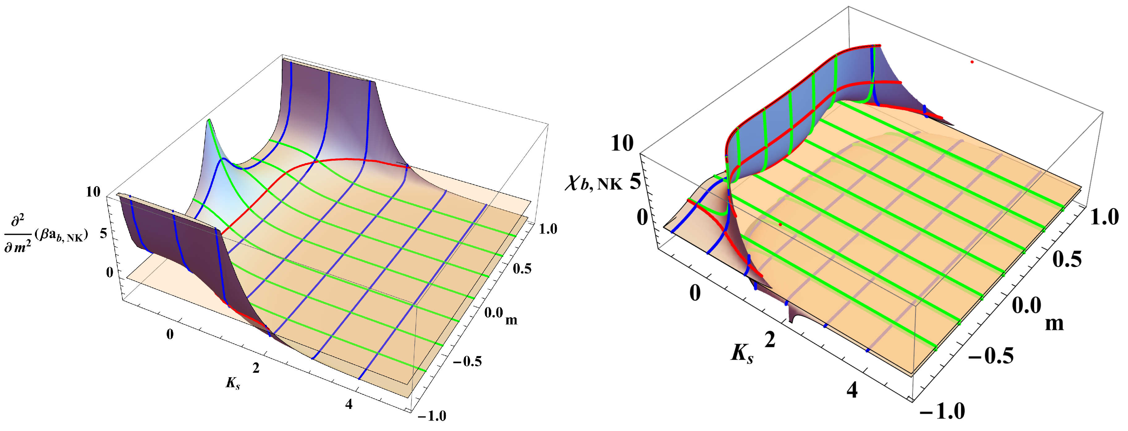
Figure 2.
Left panel The region in the space where the second derivative of the free energy of the system is non-negative is embraced by the figure presented. The upper surface of this reagion is given by the spinodal surface. Right panel The corresponding cross-sections of this region with planes at and are presented on the right panel. Their upper limiting lines are equal to , , and .
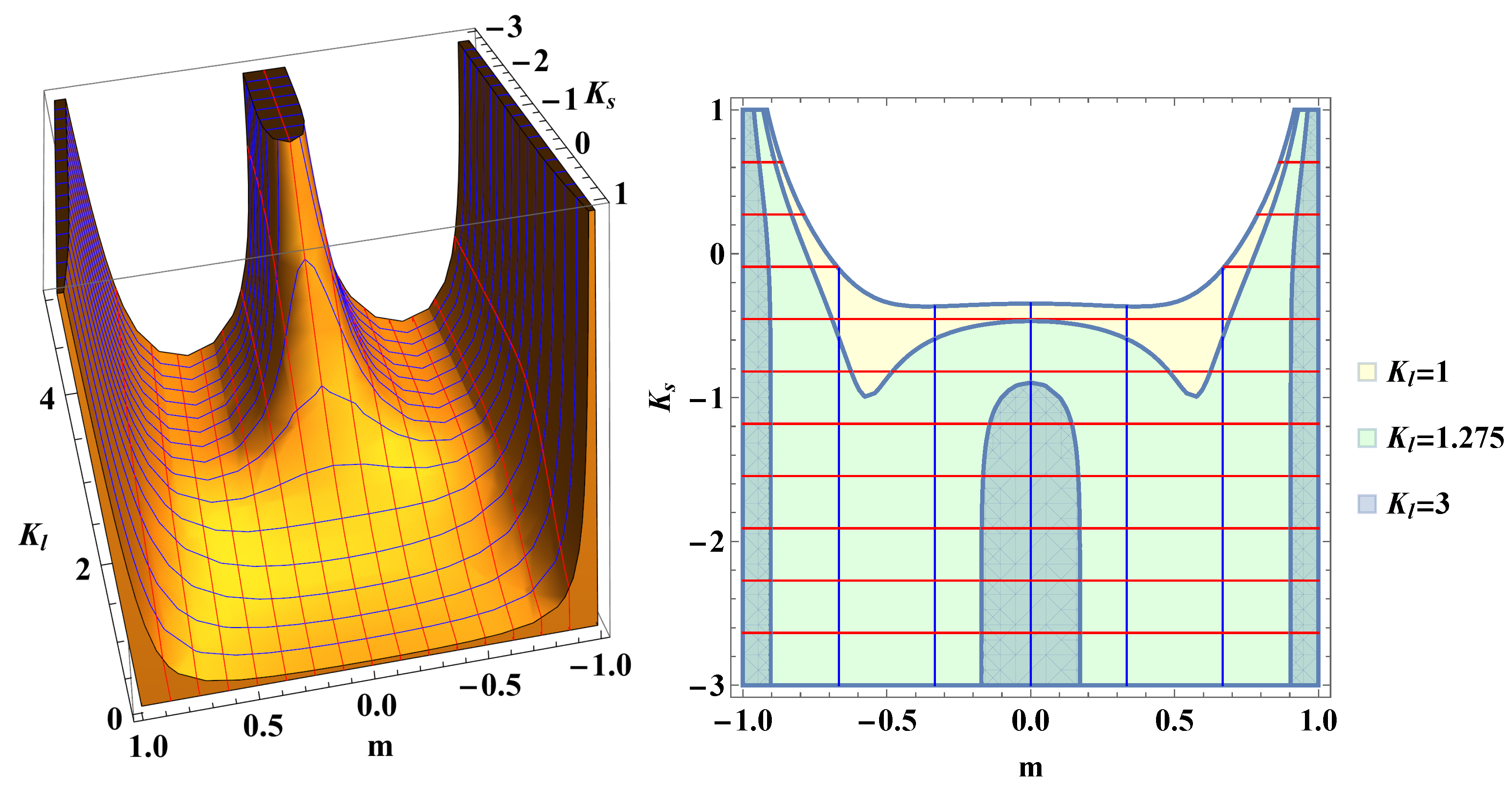
Figure 3.
The behavior of the Helmholtz bulk free energy , see Eq. (8), as a function of m for specific values of the combination and for which the system is in a thermodynamically stable (leftmost) - with convex free energy, metastable (middle), or unstable (rightmost) states - for which the free energy is concave function. For the curves of the free energy im the middle panel (in blue) there are two regions: i) region in which the free energy is concave (this is a stable region, it is about and between the orange points; these points indicate the states at which the second derivative changes its sign) and ii) another region where it is convex, i.e., the system is unstable (it is about the minimum of the free energy).
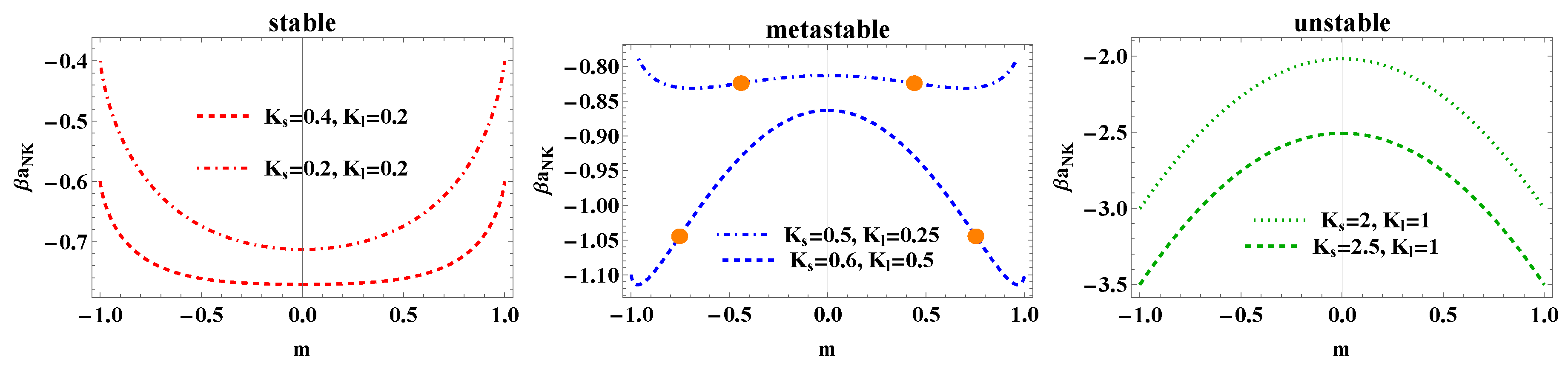
Figure 4.
Left panel The thermodynamically stable, metastable and unstable regions for Husimi-Temperley model, for which . The blues region between the dot-dashed red spinodal line of , determined by Eq. (20) with , and the dot-dashed blue line of equilibrium magnetization , given by Eq. (11) with , is the region of metastable states. The white region is the one with thermodynamically unstable states. The part of the blue region below the metastable curve is a region of stable states. Right panel The behavior of the free energy as a function of m for given values of , with .The green line has a minimum only at and the free energy is convex. That is why all states with given coordinates belonging to this curve are stable. The orange curve has a maximum at and two minima at . The curve is concave in the middle, around , and convex about . Thus, on this line we have a mixture of stable and unstable states - metastable curve. The big orange dots indicate the states at which the second derivative changes its sign. The blue line has a maximum at and minima at . This curve is everywhere concave, i.e., all states belonging to it are unstable. The vertical dot-dashed blue line on the left panel represents the solution . It is an extremum of the free energy, but it is not always its minimum — see the right panel.
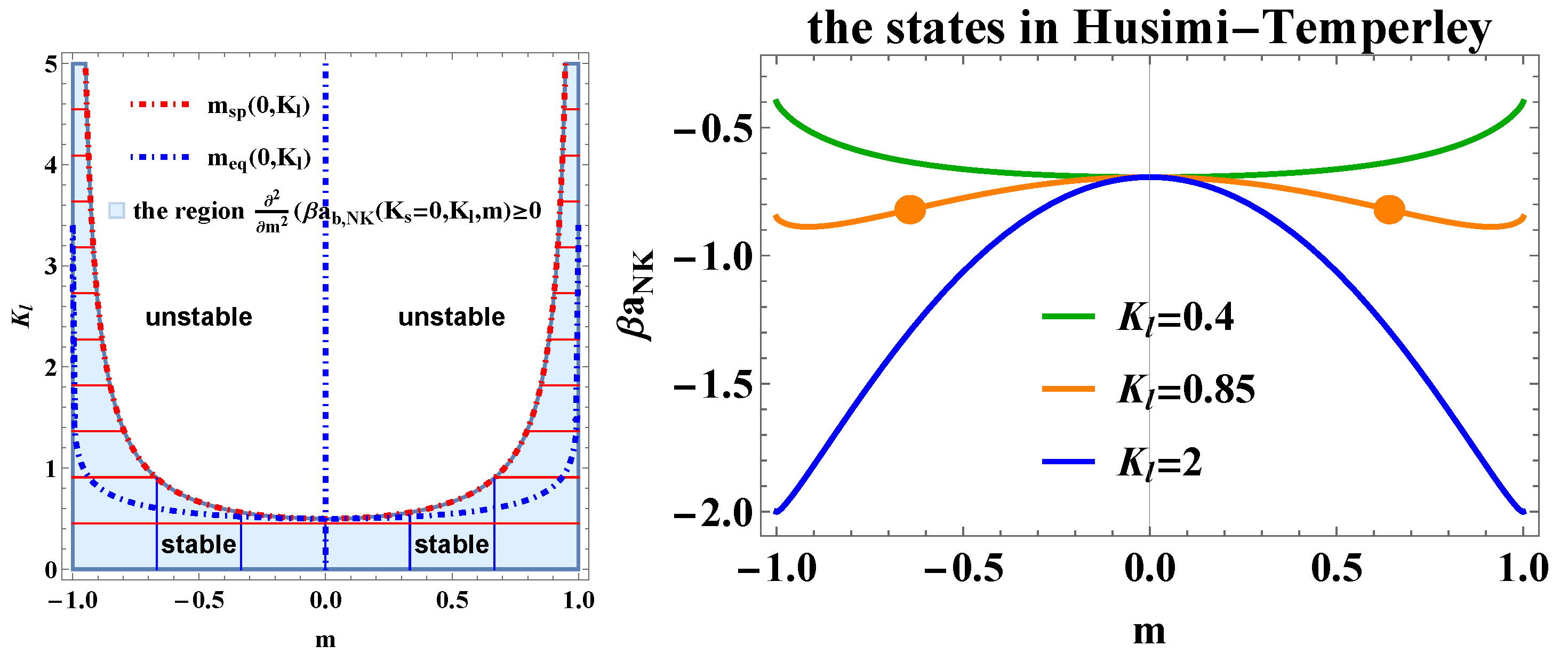
Figure 5.
The thermodynamically stable, metastable and unstable regions for Nagle-Kardar model. The reddish surface is the spinodal one, see Eq. (19), while the greenish surface is the equilibrium one, see Eq. (11). The surfaces mutually penetrate into each other. The region above the two surfaces is the one with unstable states, the one below the two - of stable states, while inbetween them embraces the metastable ones. This figure is the analogy of Figure 4, left panel, that visualizes the case of the much simpler Husimi-Temperley model.
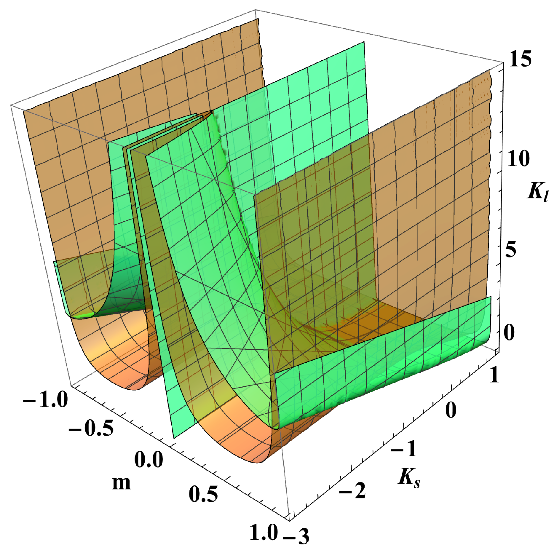
Figure 6.
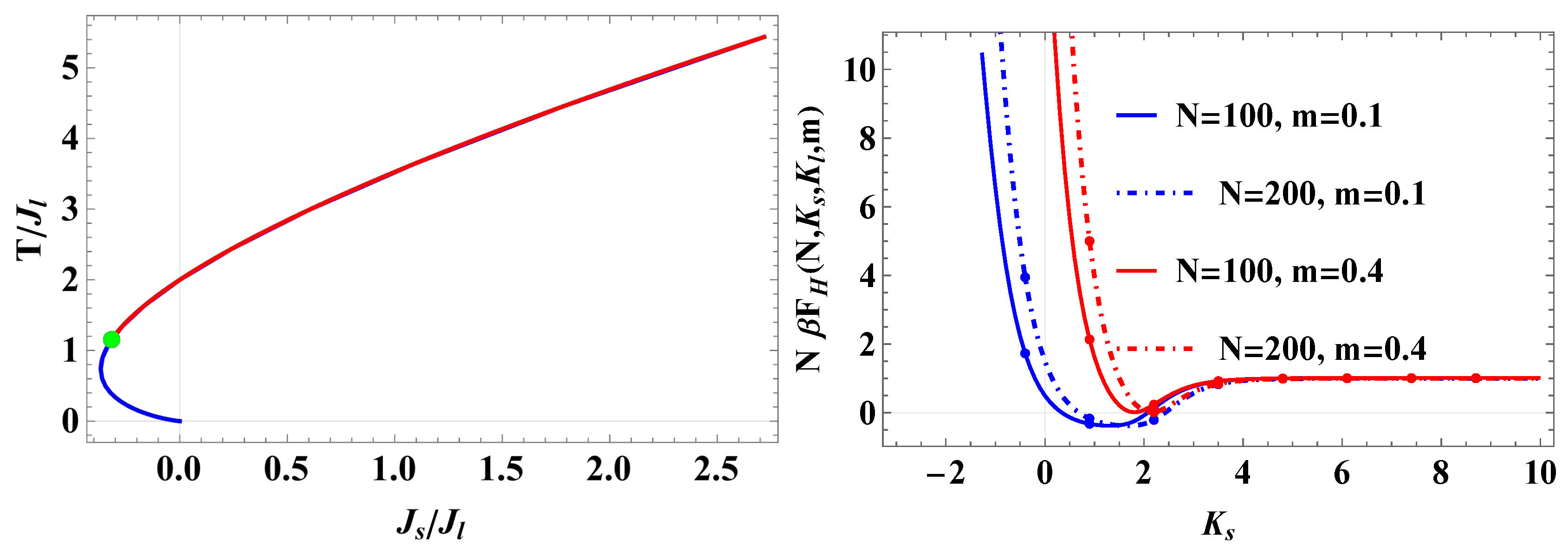
Left panel The phase diagram in terms of the temperature. It is shown as a function of and . The red line represents a line of critical points with , while the green point marks the tricritical point with . The coordinates of the tricritical point in terms of and are and in terms of and are , and . From this point, for a line is starting at which three phases with the same free energy and magnetization coexist. It is shown in blue. Above it at zero external field the magnetization is zero, while below it there are two phases with nonzero magnetization. That is why this blue line is the line of first-order phase transitions. Right panel The figure illustrates the behavior of the Helmholtz force as a function of for fixed values of N and m. This function does not depend on . The function is repulsive and increases linearly for negative values of . For large positive the curves show the usual scaling behavior of the one-dimensional Ising model. For large positive the curves show the usual scaling behavior of the one-dimensional Ising model - for details see [7,16,17,19].
Figure 6.
Left panel The phase diagram in terms of the temperature. It is shown as a function of and . The red line represents a line of critical points with , while the green point marks the tricritical point with . The coordinates of the tricritical point in terms of and are and in terms of and are , and . From this point, for a line is starting at which three phases with the same free energy and magnetization coexist. It is shown in blue. Above it at zero external field the magnetization is zero, while below it there are two phases with nonzero magnetization. That is why this blue line is the line of first-order phase transitions. Right panel The figure illustrates the behavior of the Helmholtz force as a function of for fixed values of N and m. This function does not depend on . The function is repulsive and increases linearly for negative values of . For large positive the curves show the usual scaling behavior of the one-dimensional Ising model. For large positive the curves show the usual scaling behavior of the one-dimensional Ising model - for details see [7,16,17,19].
For examples of the behavior of the bulk Nagel-Kardar Helmholtz free energy when there is the possibility of a first order phase transition, see Figure 7.
5. On the Behavior of the Helmholtz Force
Starting from the expression for the Helmholtz excess free energy
and the definition of the Helmholtz force
we obtain, with
(for some details concerning the definition of the Helmholtz force and a comparison with Casimir force see the review [7]).
From Eq. (6) and Eq. (8) we derive
The last implies that the Helmholtz force in the Nagle-Kardar model does not depend on ! In fact, it equals the Helmholtz force for the Ising model. The behavior of the force as a function of for different values of N is shown in the right panel of Figure 6. The additional essential difference with respect to the Ising model is that the critical regime in Nagle-Kardar model is not achieved, as in Ising model, for . The critical behavior is near the second-order phase transitions depicted as a red line in Figure 6.
6. Discussion and Concluding Remarks
In the current article we studied the behavior of the Nagle-Kardar model in an ensemble with conserved magnetization: the canonical ensemble, or CE. As explained in the introduction, this model has bee extensively studied in the grand canonical (with fixed external field) and in microcanonical ensemble. The current article, as far as we are aware about, is the only one that clarifies its behavior in the CE. We determined the phase diagram of the bulk model—see Figure 6. It turns out that it has the same second-oder phase transition line, ending at a tricritical point (we note that this line, using the Lambert W function, can be obtained analytically, as explained in [1]), but differs in its behavior below that point. Furthermore, it turns out that the bulk system has stable, metastable and unstable thermodynamically regions, while the model in the GCE possesses only stable states. Details about where as a function of and m these states are located are visualized in Figure 1— Figure 3. For the Nagle-Kardar model coincides with the Husimi-Temperley model, the behavior of which has been studied in both the GCE and the CE and is well known as a function of the same parameters used in the current article. This is shown in Figure 4. They are in a full agreement with the existing literature for this model. In addition to the bulk behavior, we have also studied the finite-size behavior of a Nagle-Kardar chain under periodic boundary conditions and determined the behavior of the Helmholtz fluctuation-induced force. The behavior of this force as a function of for several fixed values of the number of particles in the chain is shown in the right panel of Figure 6. Interestingly, it does not depend on , i.e., on the long-ranged part of the interaction. This means that the force actually coincides with the corresponding force for the Ising model. Thus, the Nagle-Kardar model is characterized by different thermodynamic behaviors in GCE and CE, and, in addition—by different fluctuation induced forces—the Casimir force in GCE and Helmholtz force in CE.
Author Contributions
Conceptualization, D.D., N. T. and J. R.; methodology, D.D., N. T. and J. R.; software, D. D.; validation, D.D., N. T. and J. R.; formal analysis, D.D., N. T. and J. R.; writing—original draft preparation, D.D., N. T. and J. R.; writing—review and editing, D.D., N. T. and J. R.; visualization, D.D.; All authors have read and agreed to the published version of the manuscript.
Funding
Partial financial support via Grant No KP-06-H72/5 of the Bulgarian National Science Fund is gratefully acknowledged.
Institutional Review Board Statement
Not applicable.
Informed Consent Statement
Not applicable.
Data Availability Statement
There are no data related to the study reported in the current article.
Acknowledgments
The authors thank Prof. M. Kardar for suggesting the problem and for a valuable discussion on the topic.
Conflicts of Interest
The authors declare no conflicts of interest.The funders had no role in the design of the study; in the collection, analyses, or interpretation of data; in the writing of the manuscript; or in the decision to publish the results.
Abbreviations
The following abbreviations are used in this manuscript:
| CE | canonical ensemble |
| GCE | grand canonical ensemble |
| CCF | critical Casimir force |
| PBC’s | periodic boundary conditions |
References
- Dantchev, D.; Tonchev, N.; Rudnick, J. Finite-size Nagle-Kardar model: Casimir force 2024. [arXiv:cond-mat.stat-mech/2404.18324]. [CrossRef]
- Casimir, H.B. On the Attraction Between Two Perfectly Conducting Plates. Proc. K. Ned. Akad. Wet. 1948, 51, 793–796. [Google Scholar]
- Fisher, M.E.; de Gennes, P.G. Phénomènes aux parois dans un mélange binaire critique. C. R. Seances Acad. Sci. Paris Ser. B 1978, 287, 207–209. [Google Scholar]
- Maciołek, A.; Dietrich, S. Collective behavior of colloids due to critical Casimir interactions. Rev. Mod. Phys. 2018, 90, 045001. [Google Scholar] [CrossRef]
- Dantchev, D.; Dietrich, S. Critical Casimir effect: Exact results. Phys. Rep. 2023, 1005, 1–130. [Google Scholar] [CrossRef]
- Gambassi, A.; Dietrich, S. Critical Casimir forces in soft matter. Soft Matter 2024. [Google Scholar] [CrossRef]
- Dantchev, D. On Casimir and Helmholtz Fluctuation-Induced Forces in Micro- and Nano-Systems: Survey of Some Basic Results. Entropy 2024, 26, 499. [Google Scholar] [CrossRef]
- Barber, M.N. Finite-size Scaling. In Phase Transitions and Critical Phenomena; Domb, C.; Lebowitz, J.L., Eds.; Academic, London, 1983; Vol. 8, chapter 2, pp. 146–266.
- Privman, V. Finite-size scaling theory. In Finite Size Scaling and Numerical Simulations of Statistical Systems; Privman, V., Ed.; World Scientific, Singapore, 1990; pp. 1–98.
- Brankov, J.G.; Dantchev, D.M.; Tonchev, N.S. The Theory of Critical Phenomena in Finite-Size Systems - Scaling and Quantum Effects; World Scientific, Singapore, 2000.
- Garcia, R.; Chan, M.H.W. Critical Fluctuation-Induced Thinning of 4He Films near the Superfluid Transition. Phys. Rev. Lett. 1999, 83, 1187–1190. [Google Scholar] [CrossRef]
- Garcia, R.; Chan, M.H.W. Critical Casimir Effect near the 3He-4He Tricritical Point. Phys. Rev. Lett. 2002, 88, 086101. [Google Scholar] [CrossRef]
- Ganshin, A.; Scheidemantel, S.; Garcia, R.; Chan, M.H.W. Critical Casimir Force in 4He Films: Confirmation of Finite-Size Scaling. Phys. Rev. Lett. 2006, 97, 075301. [Google Scholar] [CrossRef]
- Hertlein, C.; Helden, L.; Gambassi, A.; Dietrich, S.; Bechinger, C. Direct measurement of critical Casimir forces. Nature 2008, 451, 172–175. [Google Scholar] [CrossRef]
- Schmidt, F.; Callegari, A.; Daddi-Moussa-Ider, A.; Munkhbat, B.; Verre, R.; Shegai, T.; Käll, M.; Löwen, H.; Gambassi, A.; Volpe, G. Tunable critical Casimir forces counteract Casimir–Lifshitz attraction. Nat. Phys. 2022. [Google Scholar] [CrossRef]
- Dantchev, D.; Rudnick, J. Exact expressions for the partition function of the one-dimensional Ising model in the fixed-M ensemble. Phys. Rev. E 2022, 106. [Google Scholar] [CrossRef]
- Dantchev, D.M.; Tonchev, N.S.; Rudnick, J. Casimir versus Helmholtz forces: Exact results. Ann. Phys-New. York. 2023, 459. [Google Scholar] [CrossRef]
- Dantchev, D.; Tonchev, N. A Brief Survey of Fluctuation-induced Interactions in Micro- and Nano-systems and One Exactly Solvable Model as Example. arXiv:2403.17109 [cond-mat.stat-mech] 2024, [arXiv:cond-mat.stat-mech/2403.17109]. [CrossRef]
- Dantchev, D.; Tonchev, N.; Rudnick, J. Casimir and Helmholtz forces in one-dimensional Ising model with Dirichlet (free) boundary conditions. Ann. Phys-new. York. 2024, 464, 169647. [Google Scholar] [CrossRef]
- Baker, G.A. Ising model with a long-range interaction in presence of residual short-range interactions. Phys. Rev. 1963, 130, 1406–1411. [Google Scholar] [CrossRef]
- Nagle, J.F. Ising chain with competing interactions. Phys. Rev. A 1970, 2, 2124. [Google Scholar] [CrossRef]
- Kardar, M. Crossover to equivalent-neighbor multicritical behavior in arbitrary dimensions. Phys. Rev. B 1983, 28, 244–246. [Google Scholar] [CrossRef]
- Patelli, A.; Ruffo, S. Statistical mechanics and dynamics of long-range interacting systems. Rivista Di Matematica Della Universita Di Parma 2013, 4, 345–396. [Google Scholar]
- Campa, A.; Dauxois, T.; Fanelli, D.; Ruffo, S. Physics of long-range interacting systems, first edition. ed.; Oxford University Press: Oxford, 2014; pp. xvi, 410 p.
- Gupta, S.; Ruffo, S. The world of long-range interactions: A bird’s eye view. Int. J. Mod. Phys. A 2017, 32. [Google Scholar] [CrossRef]
- K.Husimi. Statistical mechanics of condensation. In Proceedings of the Proc. Intern. Conf. Theor. Phys. Kyoto and Tokyo, 1953, p. 531.
- Temperley, H.N.V. The Mayer theory of condensation tested against a simple model of imperfect gas. Proc. Phys. Soc. London 1954, A 67, 233. [Google Scholar] [CrossRef]
- Hoye, J.S. Spin model with antiferromagnetic and ferromagnetic interactions. Physical Review B 1972, 6, 4261. [Google Scholar] [CrossRef]
- Kaufman, M.; Kahana, M. Cayley-tree Ising-model with antiferromagnetic nearest-neighbor and ferromagnetic equivalent-neighbor interactions. Phys. Rev. B 1988, 37, 7638–7642. [Google Scholar] [CrossRef]
- Vieira, A.; Goncalves, L. One-dimensional lattice gas. Condens. Matter Phys. 1995, 5, 210–225. [Google Scholar] [CrossRef]
- Paladin, G.; Pasquini, M.; Serva, M. Ferrimagnetism in a disordered Ising-model. Journal De Physique I 1994, 4, 1597–1617. [Google Scholar] [CrossRef]
- Vieira, A.P.; Goncalves, L.L. One-dimensional Ising model with long-range and random short-range interactions. J. Magn. Magn. Mater. 1999, 192, 177–190. [Google Scholar] [CrossRef]
- Boukheddaden, K.; Linares, J.; Spiering, H.; Varret, F. One-dimensional Ising-like systems: an analytical investigation of the static and dynamic properties, applied to spin-crossover relaxation. Eur. Phys. J. B 2000, 15, 317–326. [Google Scholar] [CrossRef]
- Mukamel, D.; Ruffo, S.; Schreiber, N. Breaking of ergodicity and long relaxation times in systems with long-range interactions. Phys. Rev. Lett. 2005, 95. [Google Scholar] [CrossRef] [PubMed]
- Mukamel, D. Notes on the Statistical Mechanics of Systems with Long-Range Interactions. arXiv:0905.1457 [cond-mat.stat-mech] 2009. [CrossRef]
- Campa, A.; Dauxois, T.; Ruffo, S. Statistical mechanics and dynamics of solvable models with long-range interactions. Phys. Rep. 2009, 480, 57–159. [Google Scholar] [CrossRef]
- Bouchet, F.; Gupta, S.; Mukamel, D. Thermodynamics and dynamics of systems with long-range interactions. Physica A 2010, 389, 4389–4405. [Google Scholar] [CrossRef]
- Ostilli, M. Mean-field models with short-range correlations. Epl 2012, 97. [Google Scholar] [CrossRef]
- Salmon, O.D.R.; de Sousa, J.R.; Neto, M.A. Phase diagrams of a spin-1 Ising system with competing short- and long-range interactions. Phys. Rev. E 2015, 92. [Google Scholar] [CrossRef] [PubMed]
- Kardar, M.; Kaufman, M. Competing Criticality of Short- and Infinite-Range Interactions on the Cayley Tree. Phys. Rev. Lett. 1983, 51, 1210–1213. [Google Scholar] [CrossRef]
- Kaufman, M.; Kahana, M. Cayley-tree Ising model with antiferromagnetic nearest-neighbor and ferromagnetic equivalent-neighbor interactions. Phys. Rev. B 1988, 37, 7638. [Google Scholar] [CrossRef]
- Cohen, O.; Rittenberg, V.; Sadhu, T. Shared information in classical mean-field models. J. Phys. A 2015, 48. [Google Scholar] [CrossRef]
- Li, Z.X.; Hou, J.X. Cooling a long-range interacting system faster via applying an external magnetic field. Mod. Phys. Lett. B 2022, 36. [Google Scholar] [CrossRef]
- Campa, A.; Gori, G.; Hovhannisyan, V.; Ruffo, S.; Trombettoni, A. Ising chains with competing interactions in the presence of long-range couplings. J. Phys. A 2019, 52. [Google Scholar] [CrossRef]
- Yang, J.T.; Hou, J.X. Effect of the nearest-neighbor biquadratic interactions on the spin-1 Nagle-Kardar model. Eur. Phys. J. B 2022, 95. [Google Scholar] [CrossRef]
- Salmon, O.D.R.; de Sousa, J.R.; Neto, M.A.; Padilha, I.T.; Azevedo, J.R.V.; Neto, F.D. The spin-3/2 Blume-Capel model with competing short- and long-range interactions. Physica a-Statistical Mechanics and Its Applications 2016, 464, 103–114. [Google Scholar] [CrossRef]
- Yao, Y.C.; Hou, J.X. Phase Diagram of the Nagel-Kardar Model in the Microcanonical-Canonical Crossover. Int. J. Theor. Phys. 2021, 60, 968–975. [Google Scholar] [CrossRef]
- Campa, A.; Gori, G.; Hovhannisyan, V.; Ruffo, S.; Trombettoni, A. Computation of Microcanonical Entropy at Fixed Magnetization Without Direct Counting. J. Stat. Phys. 2021, 184. [Google Scholar] [CrossRef]
- Yang, J.T.; Tang, Q.Y.; Hou, J.X. Ensemble inequivalence in an extended spin-1 Nagle-Kardar model. Chinese Journal of Physics 2024, 89, 1325–1332. [Google Scholar] [CrossRef]
- Li, Z.X.; Hou, J.X. Cooling a long-range interacting system faster via applying an external magnetic field. Mod. Phys. Lett. B 2022, 36. [Google Scholar] [CrossRef]
- Kislinsky, V.B.; Yukalov, V.I. Crossover between short-term and long-range interactions in the one-dimensional Ising-model. J. Phys. A 1988, 21, 227–232. [Google Scholar] [CrossRef]
- Mori, T. Instability of the mean-field states and generalization of phase separation in long-range interacting systems. Phys. Rev. E 2011, 84, 031128. [Google Scholar] [CrossRef] [PubMed]
- Mori, T. Phase transitions in systems with non-additive long-range interactions. J. Stat. Mech: Theory Exp. 2013, 2013, P10003. [Google Scholar] [CrossRef]
- Abramowitz, M.; Stegun, I.A. Handbook of mathematical functions with formulas, graphs, and mathematical tables; Dover, New York, 1970.
- Kardar, M. Statistical Physics of Fields; Cambridge University Press, Cambridge, 2007.
Figure 7.
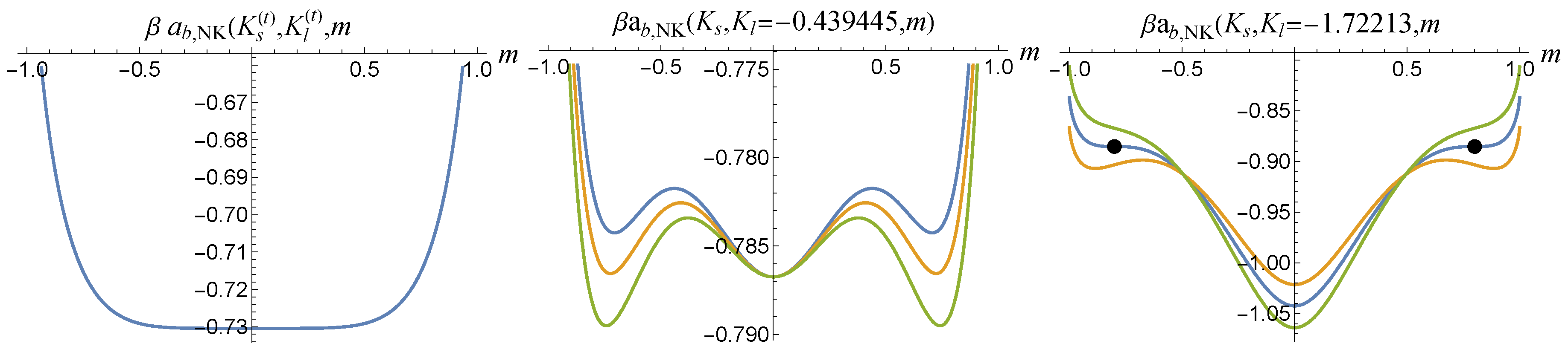
Three examples of the behavior of the bulk Helmholtz free energy in the Nagel-Kardar model, ; see Eq. (8). Leftmost panel: the free energy at the tricritical point, where is the value of at the tricritical point and is the value of there. Middle panel: The bulk Helmholtz bulk free energy with set equal to -0.439554, as indicated on the plot, and set equal to the three values -1.44, -1.4445 and -1.5. There is a first order phase transition between a state with a global minimum at and one of two states with nonzero m when (see the orange line). Rightmost panel: the bulk Helmholtz free energy with set equal to -1.72213 and equal to the three values -0.885264, -0.855264 and -0.915264. At equal to the first value (blue curve), there are spinodal points. When has the second value (orange curve) there is a metastable state at two equal and opposite values of m, and when has the third value (green curve) the only free energy minimum is at .
Figure 7.
Three examples of the behavior of the bulk Helmholtz free energy in the Nagel-Kardar model, ; see Eq. (8). Leftmost panel: the free energy at the tricritical point, where is the value of at the tricritical point and is the value of there. Middle panel: The bulk Helmholtz bulk free energy with set equal to -0.439554, as indicated on the plot, and set equal to the three values -1.44, -1.4445 and -1.5. There is a first order phase transition between a state with a global minimum at and one of two states with nonzero m when (see the orange line). Rightmost panel: the bulk Helmholtz free energy with set equal to -1.72213 and equal to the three values -0.885264, -0.855264 and -0.915264. At equal to the first value (blue curve), there are spinodal points. When has the second value (orange curve) there is a metastable state at two equal and opposite values of m, and when has the third value (green curve) the only free energy minimum is at .
Disclaimer/Publisher’s Note: The statements, opinions and data contained in all publications are solely those of the individual author(s) and contributor(s) and not of MDPI and/or the editor(s). MDPI and/or the editor(s) disclaim responsibility for any injury to people or property resulting from any ideas, methods, instructions or products referred to in the content. |
© 2024 by the authors. Licensee MDPI, Basel, Switzerland. This article is an open access article distributed under the terms and conditions of the Creative Commons Attribution (CC BY) license (http://creativecommons.org/licenses/by/4.0/).
Copyright: This open access article is published under a Creative Commons CC BY 4.0 license, which permit the free download, distribution, and reuse, provided that the author and preprint are cited in any reuse.


