Preprint
Article

This version is not peer-reviewed.

Ecosystem Health Assessment of the Zerendy District, Kazakhstan

A peer-reviewed article of this preprint also exists.

Submitted:

04 December 2024

Posted:

04 December 2024

You are already at the latest version

Abstract

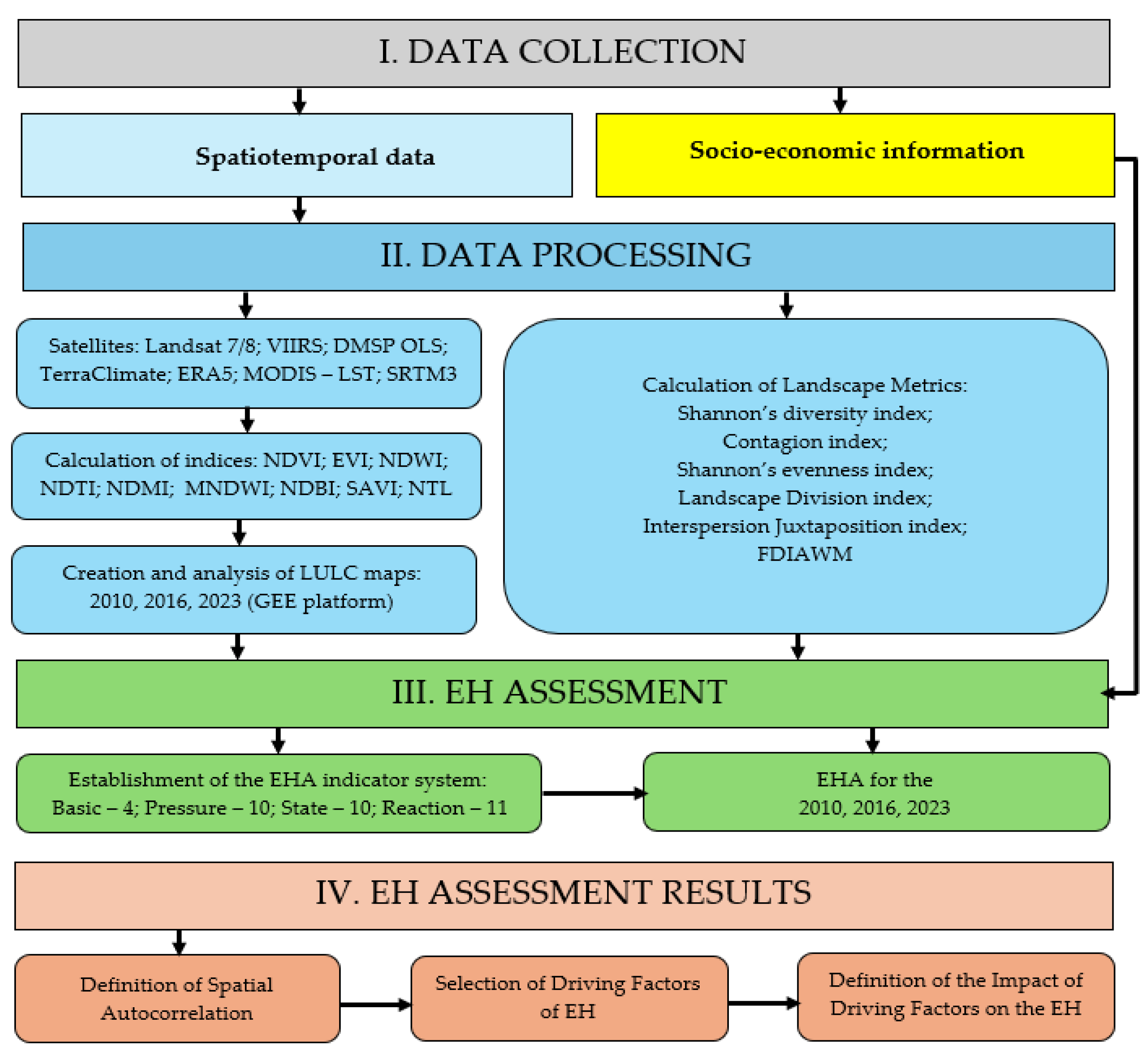
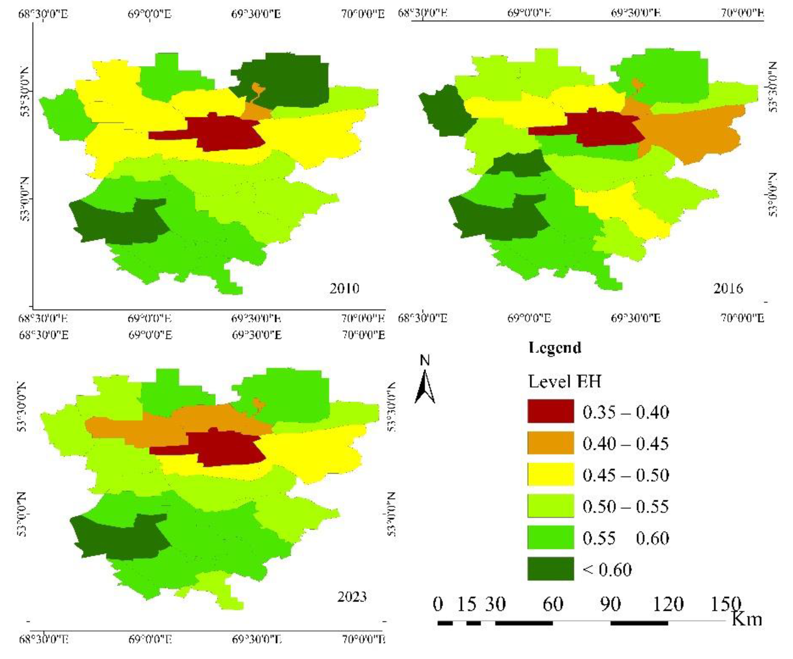
Ecosystem Health Assessment (EHA) is essential for comprehensively improving the ecological environment and socio-economic conditions, thereby promoting sustainable development of a specific area. Most previous EHA studies have focused on urbanized regions, paying insufficient attention to rural areas with urban enclaves and national natural parks. This study employed the Basic-Pressure-State-Response methodological approach. The composition of indicators (35) encompassed both spatiotemporal data and socio-economic information. The Random Forest algorithm was used on the Google Earth Engine platform to classify and evaluate changes in Land Use and Land Cover (LULC). In addition, weighting coefficients were calculated, and driving factors were subsequently identified. The analysis revealed that the rural administrative divisions in the central part of Zerendy district, where the city of Kokshetau is situated, exhibited a relatively low level of Ecosystem Health (EH). The southwestern rural administrative divisions of the studied district, where the national nature park and the reserve territories are located, exhibited a higher level of EH. Other rural administrative divisions located in the eastern parts of the district generally exhibited a moderate level of EH. Interested managers can use the results of our assessment to implement adequate measures aimed at improving the health of the Zerendy district ecosystem.

Keywords: 
;  ;  ;  ;  ;  ;  ;  ;  ;  ;  ;  

1. Introduction

Despite specific difficulties that have arisen in the schedule of the 2030 Agenda, the Sustainable Development Goals (SDGs) are still within reach, but more efforts are required [1]. One of the areas of effort should be research aimed at identifying the internal patterns of “sustainable development”, which can contribute to the earliest possible achievement of the 2030 SDGs. At the same time, despite the passage of more than three centuries since the concept of “sustainability” emerged and the adoption of 17 SDGs, the discussion on the internal structure of “sustainable development” [2,3,4,5] continues. For example, epistemological studies have shown that concepts such as sustainability, resilience, adaptation, transformation, vulnerability and innovation require further understanding and clarification of their application areas [6,7,8,9,10,11]. Importantly, these concepts provide additional information that serves as a basis for developing new approaches and strategies for implementing the SDGs. They also enable the prediction of future research directions in the field of sustainable development [12].
One concept contributing to achieving SDG 2030 is Ecosystem Health (EH), a product of interdisciplinary research [13]. Its aim is to improve the health and well-being of people, animals, and ecosystems and is partly based on the principle of sustainability [14]. The development of EH dates back to 1941. However, despite the constant enrichment and development of the EH concept, there is still no generally accepted definition [15,16,17,18,19,20]. EH is expected to support the stability and integrity of the ecosystem’s internal structure and function, ensure resilience and recovery under external pressures, and provide normal service functions to meet the needs of human social development [20]. According to [21], EH is a relative concept where the relative health of an ecosystem is measured in a specific spatial location and over time. EH combines natural and social sciences [22,23,24,25]. It is believed [24] that achieving EH should become the cornerstone of sustainable development policy, as maintaining it is the main factor in achieving sustainable socio-economic and environmental development. According to [13], research in the field of EH has gone through the stages of anthropocentrism and biocentrism and is currently based on ecocentrism. EH has gradually become an essential issue of our time, as evidenced by the rapid increase in publications on EH over the past ten years [13,26,27]. Several organizations [28,29,30], including individual divisions of the UN [25], and many researchers from different countries and schools are directly involved in the development of EH.
EH requires continuous determination and assessment of its condition [31]. Therefore, the current focus of research has shifted to the methods of EH Assessment (EHA) [15] and the development of its indicators [31]. Various approaches are used for EHA, which can be divided into two large groups: the biological indicator method and the index system method [15]. The first method is based on the use of individual indicator organisms. Due to the lack of information on such indicators, this paper does not consider the biological indicator method. The second method uses indicators combined with socio-economic data, determines their weights and forms a complex index for EHA. Therefore, the index system method is the focus of this paper.
Index systems have been created to synthesize complex information to reflect the actual situation on EH. The prototype of the index method can be considered Vigor, Organization, and Resilience (VOR) [32]. Based on this idea, researchers developed Vigor, Organization, Resilience, and Stability (VORS) [33] and Vigor, Organization, Resilience, Ecosystem Services, and Stability (VORES) [34] and further enhanced it by constructing optimized and improved subindices [35]. The next most frequently used model is the Pressure-State-Response (PSR) model [17,19,36,37] proposed by the Organisation for Economic Co-operation and Development (OECD) [38]. The PSR model is also subject to development. For example, its modifications such as Driving Forces-Pressure-State-Response (DFSR) [20], Driving Forces-Pressure-State-Impact-Response (DPSIR) [39,40,41], Driving Forces-Pressure-State-Impact-Response-Management (DPSIRM) [42], Driving Forces-Pressure-State-Change-Response (DPSCR) [43], Driving Forces-Pressure-State-Exposure-Effect-Action (DPSEEA) [44] and Basic-Pressure-State-Response (BPSR) [19] have been developed. At present, other EHA models have been created. These are Technique for Order Preference by Similarity to Ideal Solution (TOPSIS) [45] and Backpropagation Neural Network (BPNN) [46], which were improved to Genetic Algorithm-Backpropagation Artificial Neural Network (GA-BPANN) [47]. However, it is difficult to give preference to one of these models since, so far, no researcher has used two or more different methods for EHA in the same area on the same time scale [15]. At the same time, all other things being equal, the VOR and PSR methods are improving most rapidly, but as we see from the above, the development of PSR is more intensive. This served as the basis for using the latest modification of PSR in this study – BPSR, which significantly facilitates the comprehensive assessment of the health of the regional ecosystem [19].
One of the disadvantages of the index system is that it is considered to be ignoring detailed information [15]. It is believed that local or regional EHA should focus on studying its temporal and spatial differences [48]. According to [17], each model of the index system is only a basic organizing paradigm for assessing the state of EH. Because each ecosystem has indicators that reflect various aspects of its health, the EHA example, with EHA, cities can use environmental and production functions as internal and economic indicators as external indicators [50].
After establishing an appropriate index system, the Ecosystem Health Index (EHI) is calculated based on the weight assigned to each metric. The choice of weighting method leads to varying ranges of EHI. As for the definition of the indicators, it has been established that there is no uniform standard of EHA. It is determined based on the understanding and interpretation of the connotation of the concept of “ecosystem health” in combination with the results of previous studies and the specific types of ecosystems selected by the researchers, which is entirely subjective [13]. In this case, researchers usually adhere to the principles of integrity, simplicity, and dynamic response, which are not indicators but macro dimensions. Within the framework of macro dimensions, it is relatively easy to understand the drivers of EH, which are social, economic, and environmental indicators [51].
The object of our study is the Zerendy district, a conglomerate of three critical territories. First, it is a city of oblast significance, which is an enclave of this Area of Interest (AOI). Next are the rural divisions of the district engaged in agro-industrial activities, which are the most minor units for which statistical information is collected on a national scale. In addition, a significant part of the territory of the Zerendy district is occupied by a natural national park and a nature reserve or protected areas. Therefore, the direction of our research on EHA is unique due to the coverage of the territory for different target purposes. (Figure 1).
In EHA, of the three areas mentioned, researchers have paid more attention to cities due to their essential role in economic development and the accompanying deterioration in the quality of the urban environment in the context of rapid urbanization [35,50,52,53,54,55,56,57,58].
The peculiarity of rural EHA is that they include a vast diversity. When studying rural health, they are often divided into disciplinary boundaries, which limits the understanding of the health of rural ecosystems as a whole. The many connections between soils, plants, animals and people related to health challenges all monodisciplinary health studies in agricultural ecosystems. Therefore, an interdisciplinary approach is necessary for a more integrated and comprehensive understanding of rural ecosystem health [59,60]. Such studies on EHA for rural regions have typically covered large regions [17,33,61,62,63,64]. However, we have not found any studies that have examined the EHA of the most minor subunits of administrative-territorial divisions, which are below the rural district – such as rural subdivisions.
Of considerable interest are the EHA of territories occupied by national natural parks [65,66], which are divided into strictly protected zones and zones for economic purposes, where work is carried out that is necessary for the functioning and development of the national natural park, as well as the provision of socio-economic infrastructure [67].
Based on the above, the goal of our research was the EHA of the Zerendy district through the construction of a conceptual model based on the BPSR structure and the research objectives:
- identifying changes in individual LULC classes;
- compiling a set of indicators corresponding to the BPSR model;
- performing EHA of individual administrative-territorial divisions of the district;
- analyzing the spatial dependence of the main clusters;
- Identify the main driving forces influencing the district’s EH.

2. Materials and Methods

2.1. Study Area

Zerendy district is located in the north of the Akmola Region of Kazakhstan (52°33′–53°40′N, 68°28′–70°4′E). It includes 22 rural districts (Figure 2) [68], which occupy the third tier in the republican administrative-territorial structure after the oblast and district [69]. Socioeconomic data are collected on them, which can be used for EHA.
The city of Kokshetau is an enclave surrounded by the territory of the Zerendy district and serves as the Centre of the Akmola oblast [70]. The city of Kokshetau is not administratively part of the Zerendy district. However, in this study, the Zerendy district and the city of Kokshetau are considered a single space for assessing the EH since the impact of the city on rural areas is inevitable. The territory of the Zerendy district is located on the western edge of the Kazakh folded country [73], where a relief is characterized by a low-mountain lowland plain. The hydrographic network of the district includes the rivers Shagalaly and its right tributary, Kylshykty, which flow from south to north. In the south of the district, the rivers Zhabay, Arshaly, and Koshkarbay originate from the Ishim River basin. There are also many small lakes in the district territory [71]. The district’s climate is continental, with long, low-snow winters and dry, warm summers. The average temperature in January is (−18°C), and in July (+19°C). The average annual precipitation varies from 350 to 400 mm. Snow cover lasts 140-160 days, but its average height is only 20 cm [74]. The Zerendy district and its enclave uniquely combine urbanized, agricultural and nature conservation areas. The city of Kokshetau, as well as the Kokshetau National Park and the Zerendy Zoological Reserve (Figure 3), have a significant impact on the ecosystems of the district.
If the city’s anthropogenic impact is a pressing concern, the national park and the reserve, in stark contrast, are actively working towards the preservation and restoration of the district’s ecosystem. In general, the heterogeneity of the natural and socio-economic conditions of development in different parts of the district makes it a unique object for EHA.

2.2. Methods

For EHA, we adopted BPSR [19] as the base method. The study was divided into four stages, shown in Figure 4.

2.2.1. Data Collection

Data collection for this study was conducted in two directions. The first direction was spatiotemporal data, including meteorological data classified by LULC classes from Landsat 7/8 images and landscape metrics. The second direction was socioeconomic statistical information by administrative-territorial divisions.

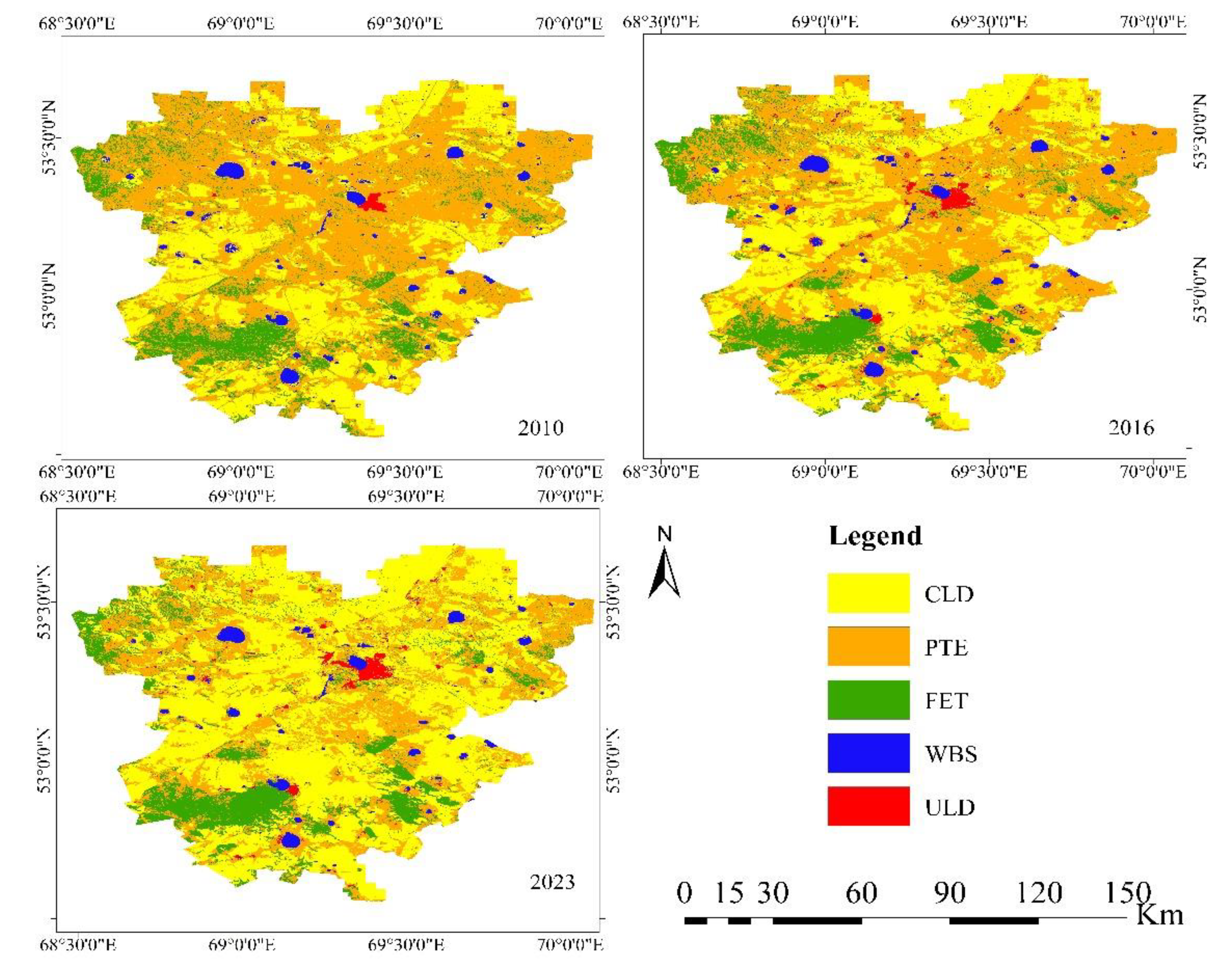
2.2.2. Data Processing

Satellite data from the Earth Engine Data Catalog [75] were used to obtain the spatiotemporal data. Some of their characteristics are given in Table 1.
2.2.2.1. Land Use and Land Cover Classification
Landsat 7/8 images were used to analyze the LULC changes from 2010, 2016 and 2023. The LULC was classified into five classes:
1)
>1) Cropland - CLD,
2)
>2) Pasture - PTE,
3)
>3) Forest - FET,
4)
>4) Water Bodies -WBS,
5)
>5) Urban Land – ULD
using the RF algorithm on the Google Earth Engine (GEE) platform. To improve the classification accuracy were used the following indices: NDVI, EVI, NDWI, NDTI, NDMI, MNDWI [76,77,78,79,80,81], as well as NLT [82], which are described in detail in our previous studies [83,84].
2.2.2.2. Landscape Metrics
Data related to landscape change measures such as Shannon’s diversity index, Contagion index (%), Shannon’s evenness index, Landscape Division Index, Interspersion Juxtaposition Index, and FDIAWM were calculated in Fragstats 4.2 software [85].
2.2.2.3. Statistical Information
The statistical data on administrative-territorial divisions that we used in our study were obtained from the Yearbook of the Bureau of National Statistics Agency for Strategic Planning and Reforms of the Republic of Kazakhstan [86].

2.2.3. Ecosystem Health Assessment

To calculate the EH level, the BPSR system [19] was used, which organizes indicators into four different but interrelated categories: B (Basic), P (Pressure), S (State) and R (Response). In this study, B is the degree of impact of climatic factors, P is the level of pressure exerted by anthropogenic and natural factors on the study area, S characterizes the state of the ecosystem, and R describes the response to pressure. All BPSR indicators we collected and their weighting coefficients are presented in Table 2.
Ecosystem resilience (Rs) was assessed based on the area occupied by LULC classes and calculated using the following formula [87]:
R s = k = 1 m P k × E C k
where P k _k is the area of the class in the district, and E C k is the ecosystem elasticity coefficient of the given class.
Based on studies [88], the ecosystem Elasticity coefficient (EC) of the classes was measured using the following equation:
EC=0.7×Resist+0.3×Resil
where EC denotes the ecosystem elasticity coefficient; ’Resil’ refers to the Resilience coefficient of the LULC class, and ’Resist’ refers to the Resistance coefficient of the LULC class.
In this study, more emphasis was placed on Resistance, as the area occupied by Cropland expanded rapidly, increasing interventions and disturbances. Therefore, greater weight was assigned to Resistance (0.7) and less to Resilience (0.3). The coefficient applied for each land-use type is listed in Table 3.
Given the differences in measurement and scale of the selected indicators, the data were standardized [89] before analysis using the following equations:
For positive indicators:
  X i j = x i j m i n ( x j ) m a x ( x j ) m i n ( x j )
For negative indicators:
X i j = max x j x i j m a x ( x j ) m i n ( x j )
where X i j is the normalized value of indicator j in year i, x i j represents the value of indicator j in year i; max x j and m i n ( x j ) , denote the maximum and minimum values of indicator j overall years, respectively. All index values range from 0 to 1.
2.2.3.1. Determination of Indicator Weights
This instrument uses the entropy method to determine weighting factors, which measure the uncertainty or variability of data. The greater the variability indicator, the greater its weight. The entropy method allows for an objective consideration of the originality of data and the depreciation of outlier estimates. In addition, this method can correct for limitations associated with the relationships between indicators, making it more efficient and practical [90]. Calculating weighting factors using the entropy method consists of the following steps:
1) Calculation of the share of indicator j in year i:
P i j = X i j i = 1 n X i j , ( i = 1 , 2 , , n ; j = 1 , 2 , , m )
2) Calculating the entropy level of the index j:
I E j = k i = 1 n P i j ln P i j , k = 1 l n ( n ) , I E j 0
3) Calculation of the difference coefficient for the indicator j:
C j = 1 I E j
4) Calculation of the weight of the indicator j:
W j = C j j = 1 m C j , j = 1 , 2 , , m , j = 1 m W j = 1
where P i j the share of indicator j in the year i, X i j is the value of indicator j in the year i, I E j is the entropy of indicator j, C j is the difference coefficient of indicator j, W j is the weight coefficient of the indicator.
2.2.3.2. Calculation of EH Using of Indicator Weights
The calculation of the ecosystem health level was carried out according to the following formula [91]:
                      E H i = n W j × X i j ( j = B 1 , B 2 , B 3 , A ^ A ^ A ^ , R 9 )
where E H i is the ecosystem health level for year i, W j is the weighting coefficient of category j, X i j is the normalized value of indicator j for year i.
In turn, the values of the BPSR categories are calculated using the following formulas [19]:
B i = j = B 1 n W j × X i j ( j = B 1 , B 2 , B 3 , B 4 )
                    P i = j = P 1 n W j × X i j ( j = P 1 , P 2 , P 3 , A ^ A ^ A ^ , P 7 )
                  S i = j = S 1 n W j × X i j ( j = S 1 , S 2 , S 3 , A ^ A ^ A ^ , S 10 )
              R i = j = R 1 n W j × X i j ( j = R 1 , R 2 , R 3 , A ^ A ^ A ^ , R 9 )
where B i , P i , S i , R i are the category values taking into account the weighting coefficient for year i, W j is the weighting coefficient of indicator j, X i j is the normalized value of indicator j for year i.

2.2.4. Analysis Methods and Spatial Correlation Indicators for EH

Moran’s I Index

The Moran’s I Index is used in this study to identify the characteristics of spatial autocorrelation. It allows us to determine whether there are spatial patterns in the data, such as clustering of high or low values of the indicators, and whether one value influences neighbouring values [92].
In calculating Moran’s I index, spatial relationships were defined based on (CONTIGUITY_EDGES_ONLY) only neighbouring polygon features that share an adjacent boundary or overlap. The global Moran’s I index and LISA calculations were performed in the ArcMap software environment version 10.8.
The formula for calculating the global Moran’s I index [93]
I = n S 0 i = 1 n j = 1 n ω i , j z i z j i = 1 n z i 2
where z i is the deviation of the attribute for object i from its mean value (xi – X ¯ ), ω i , j i s the spatial weight between objects i and j, n is equal to the total number of objects, S0 is the set of all spatial weights, which in turn is equal to:
S 0 = i = 1 n j = 1 n ω i , j
To analyze clusters, outliers and their distribution, Local indicators of spatial association (LISA) were used using ArcMap version 10.8. The formula for LISA [94]:
                                                              I i = x i X ¯ S i 2 j = 1 , j i n ω i , j ( x j X ¯ )
where x i is a numeric attribute of object i , X ¯ is the mean value for this attribute, ω i , j is the spatial weight for the pair i and j, and:
S i 2 = j = 1 , j i n ( x j X ¯ ) 2 n 1
where n corresponds to the total number of objects.

Application of Principal Component Analysis

Principal component analysis (PCA) was used to identify the main factors influencing the health of ecosystems. This method allowed us to reduce the number of original variables to two key components that best reflect the variability of the data [95]. The analysis included 11 variables: population density, agricultural land area per capita, built-up area, pollutant emissions, cultivated green land area, NDVI, SAVI, NDMI, EVI, NDWI indices and waste disposal costs. PCA was performed using IBM SPSS software.
Based on the identified components, a regression model was constructed to predict the EH level. This approach takes into account the influence of independent variables, which ensures accurate modelling and understanding of how various factors affect EH.
The regression equation is as follows:
E H = δ + α 1 F 1 + α 2 F 2 + + α n F n
where α 1 , α 2 , , α n _nare the coefficients that determine the contribution of each component, F 1 , F 2 , , F n _nare the principal components obtained as a result of PCA, and δ is a constant term of the equation. The regression analysis was performed using IBM SPSS software [96].

3. Results

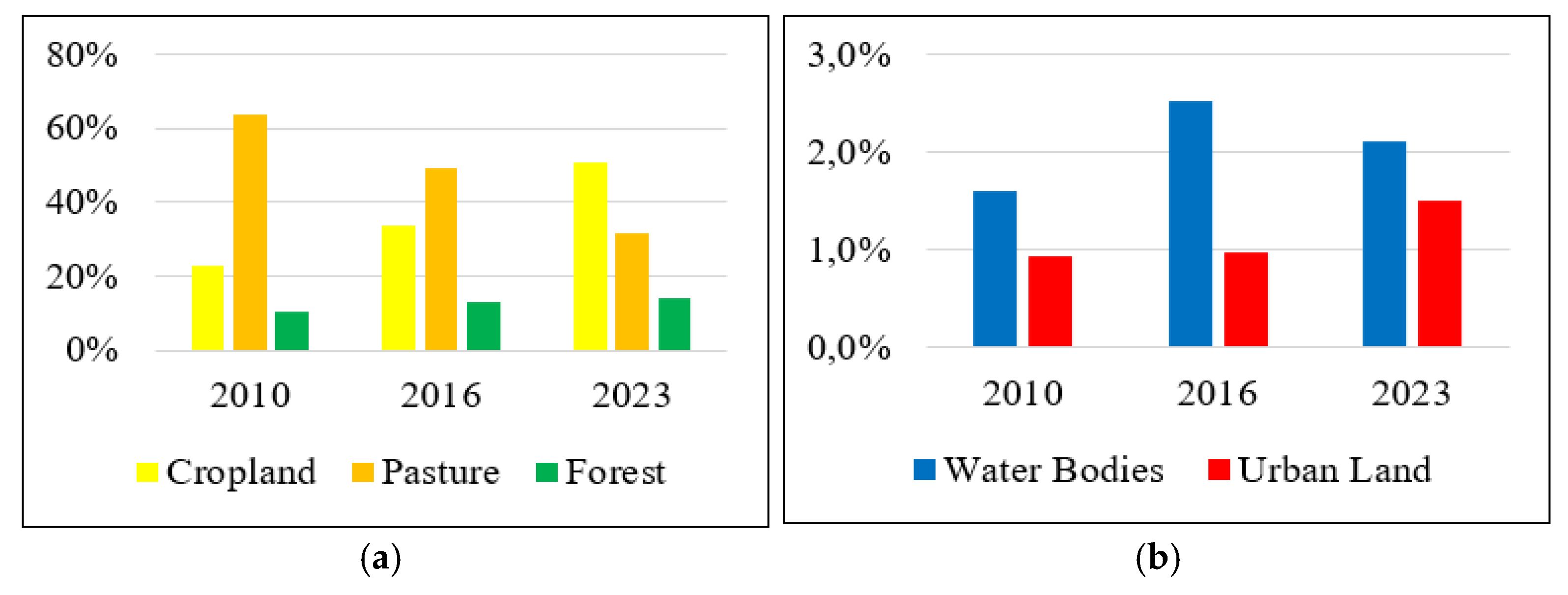
3.1. Analysis of Land Use and Land Cover Dynamics in the Zerendy District

Significant changes in LULC have occurred in the study area, which can be easily seen from Figure 5 and Table 4.
By 2023, the dominant class in the Zerendy district becomes CLD, replacing PTE and occupying 50.62% of the district area. The overall growth of the CLD class was 27.72% of the total district area from 2010 (22.90%) to 2023 (50.62%).
The leading class in terms of total area change is PTE. The PTE class has been losing areas throughout the period. It has the most significant percentage of lost area, 32.41% of the total area of the district, which cannot but affect the state of the ecosystem.
The FET class has growth dynamics and has increased its area from 2010 (10.57%) to 14.19% per cent in 2023. Thus, the total growth of the class from the initial area was 34.24% for the entire period.
WBS and ULD are the most minor classes in the area. WBS has shown a slight increase, which may be due to seasonal changes. Despite its small area, the ULD class is also characterized by a constant increase. By the end of the observation, its increase from the initial area reached 59.57%. More clearly, the trends in the change of LULC classes are shown in Figure 6a and Figure 6b.

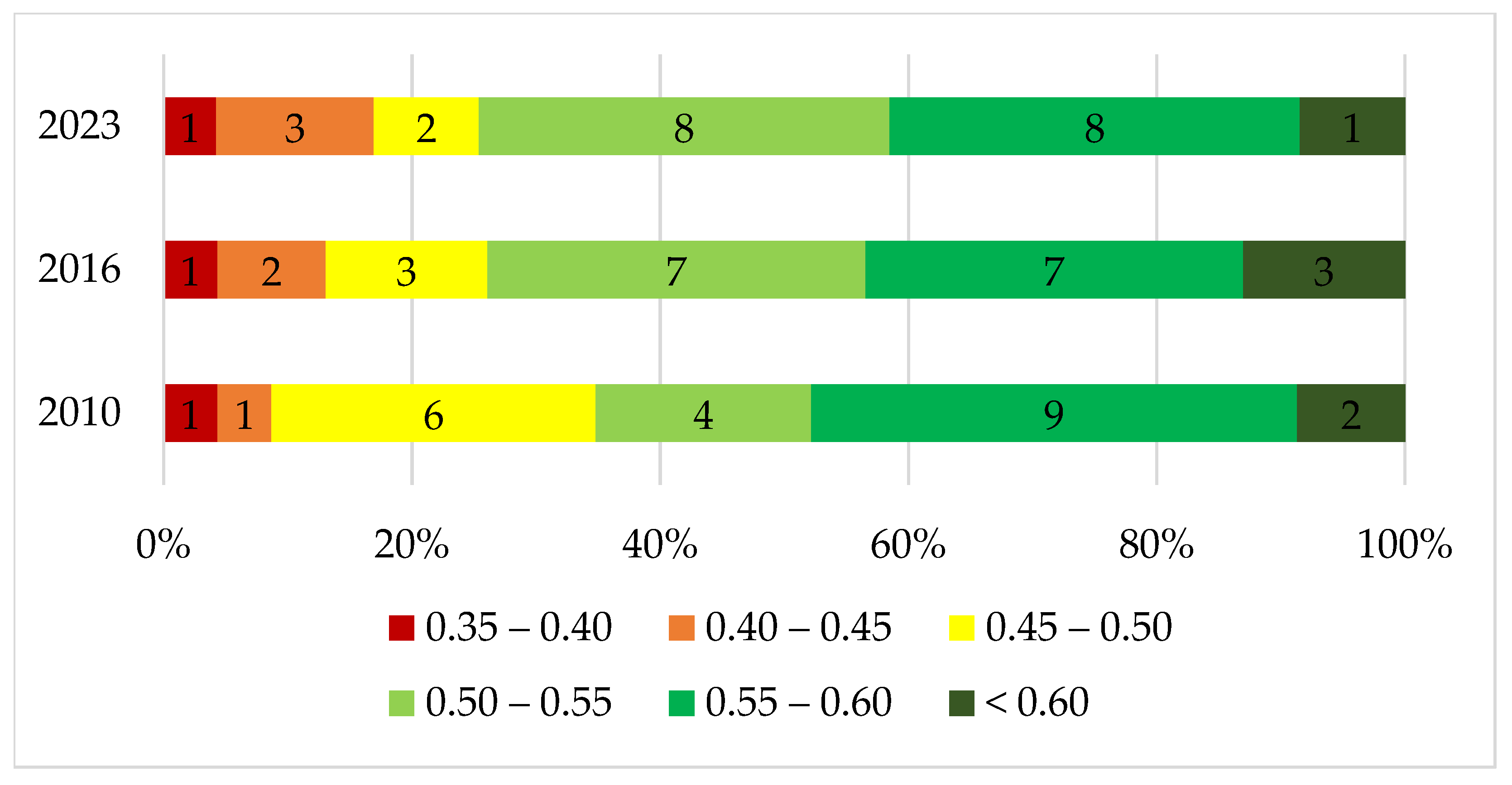
3.2. Spatiotemporal Changes in Ecosystem Health in the Zerendy District

AOI is characterized by noticeable changes in the level of ecosystem health over the period under consideration (Figure 7).
The results of the calculated EH are presented in Table 5.
We have identified 6 EH levels for the Zerendy district: very low level (1-VL), low level (2-L), medium-low (3-ML), medium (4-M), medium-high (5-MH), high (6-H). In 2010, most counties were at a relatively good level of EH: approximately 70% of counties reached 3-ML and above. In particular, Kokshetau had a level of 1-VL (0.37). The counties of Aidabol (0.59) and Sarozek (0.60) were at 5-MH, while Baiterek (0.69) reached 6-H. By 2016, some areas had seen improvements in the ecosystem. For example, in Prirechnoye, the EH level increased from 0.52 to 0.63, and in Sadovoye, from 0.47 to 0.59. However, despite these improvements, Kokshetau’s EH remained at 1-VL (0.38), and in Konysbay, it began to decrease from 0.47 to 0.42. In 2023, the EH condition worsened. The number of 2-L divisions increased. For example, these are Kyzylsaian (0.55) and Kanai Bi (0.55), which moved from 3-ML to 2-L. The average EH values over the entire observation period showed slight fluctuations. In 2010, it was 0.533; in 2016, it increased slightly to 0.542; and in 2023, it decreased again to 0.530. This indicates a general trend towards deterioration of the ecosystem condition in the AOI despite temporary improvements in individual counties.
Figure 8 illustrates these changes, showing the redistribution of EH across divisions for 2010, 2016, and 2023.
The change in the EH level during the period under consideration had different characteristics in the divisions of the Zerendy district. The center of the district, including Kokshetau, is characterized by a low EH level (from 0.35 to 0.40), while the divisions surrounding Baiterek, which are located within the boundaries of the Zerendy reserve, demonstrate a high EH level (more than 0.55).

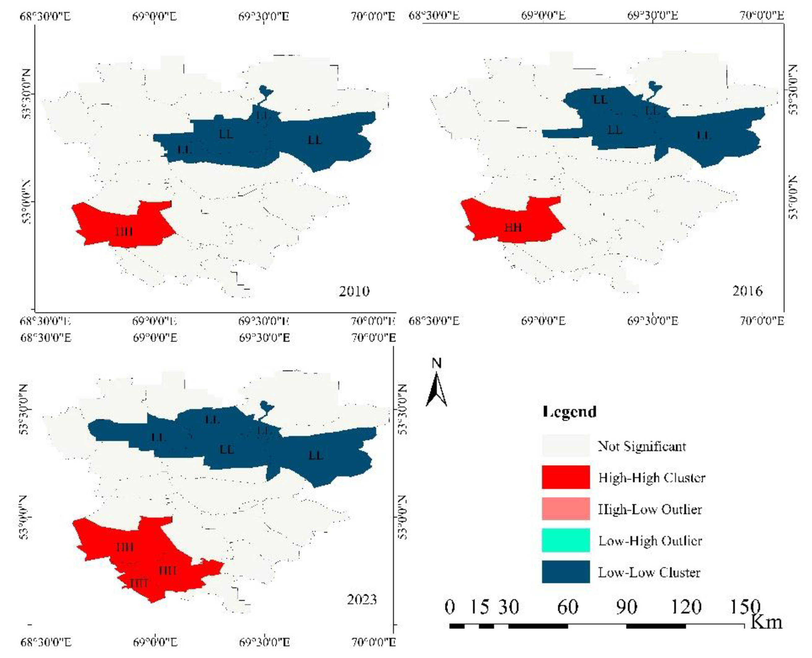
3.3. Spatial Dependence of Ecosystem Health of Zerendy District

Quantitative measurements of spatial autocorrelation of the ecosystem health level of the Zerendy district using the global Moran’s I index showed that its values in the studied years (2010, 2016, 2023) ranged from 0.42 to 0.59 (Table 6). This indicates a significant spatial autocorrelation of the ecosystem health level in the AOI. That is, the ecosystem health level in each division is under the positive or negative influence of neighbouring territories.
Regarding time dynamics, the global Moran’s I index decreased towards the middle of the period and increased towards the end. Its value decreased from 2010 to 2016, indicating a reduction in the spatial dependence of ecosystem health and a tendency towards disaggregation. From 2016 to 2023, the index value increased significantly, reflecting a relatively high spatial aggregation of ecosystem health. This may be due to the effectiveness of the district development strategy adopted after the COVID-19 recession. The Z-score is significantly higher than zero in all years, indicating the presence of spatial autocorrelation in each year. At the same time, the P-values are extremely low in all cases (less than 0.01), confirming the statistical significance of the results and the low probability of random distribution. The variance remains relatively stable throughout the years, indicating the reliability of the measurements.
Figure 9 shows the results of using LISA to study local spatial autocorrelation and analyze spatial aggregation existing in the divisions of the Zerendy district. Local autocorrelation is primarily represented by clusters of high values, designated as High-High (HH), and clusters of low values, defined as Low-Low (LL). These types of clusters indicate clusters where high and low EH values tend to concentrate in certain territories. At the same time, such types as High-Low (HL) and Low-High (LH), which are characterized by the presence of abnormal values (low values among high or high among low), are not found in the AOI. This indicates a low degree of mixed influences between high and low values of the level of ecosystem health near each other.
The HH type is the primary agglomeration type in the southwestern part of the district, indicating a concentration of divisions with high levels of ecosystem health. The prominent clustering is observed around the Zerendy Reserve and the Baiterek division. This clustering has been increasing over time. Она, especially noticeable in 2023. The LL type is mainly represented in the central and eastern parts of the region, indicating low values of ecosystem health in these regions. Districts with low EH values surround Kokshetau, the oblast’s center. In 2010, clustering in the central part was less pronounced, but by 2023 it had significantly increased. Thus, the LISA analysis shows that in the Zerendy district, there are clear groups with similar values of ecosystem health. This means that areas with high and low values are located next to each other. This is especially noticeable in the central part of the district, where the values are low, and in the southwestern part, where the values are high.

3.4. Identifying the Role of Individual Factors in Ecosystem Health of Zerendy District Based on Principal Component Analysis

PCA analysis concentrated information on changes in eleven key indicators into two principal components (Table 7).
The first principal component (F1) is a characteristic of economic development, mainly reflecting changes in population density, share of built-up area, emissions of pollutants, and pasture area. The second principal component (F2) is a characteristic of climate change, mainly reflecting vegetation indices such as NDVI, SAVI, NDMI, EVI, and NDWI.
A model of statistical relationships between changes in EH levels and principal components was obtained using regression analysis. The results of the regression model are presented in Table 8.
The R2 value shows that the model explains 72.4% of the variability in the EH level based on the principal components. This indicates a high degree of explanatory power of the model. The significance of the model (p < 0.001) also confirms the statistical significance of the obtained results. The EH level showed a negative relationship with the economic development component (F1) and a positive relationship with the climate change component (F2). This indicates that economic development hurts ecosystem health, while climate change, reflected in vegetation indicators, has a positive effect.

4. Discussion

4.1. Selection of Ecosystem Health Assessment Model

The EHA methodology began with developing the Ecosystem Distress Syndrome [97] and the Environmental Degradation Syndrome [98] or EDS models. These models describe in some detail the influence of internal natural factors on an ecosystem without assessing the influence of external factors, especially those emanating from human activities. Since human activity is the main factor threatening ecosystems [99], EHA models were further developed that consider anthropogenic activity – VOR, PSR and others. The VOR model and its modifications are more advanced than the EDS model since EHA is implemented on the vigour, organisation, and resilience framework. At the same time, the VOR, in its initial version, ignored the driving force of the current state and the ecosystem’s response to this driving force. The PSR model captures the interaction between the environment and anthropogenic activities. PSR views human activities as playing a central role in determining the state of the environment and better reflects the essence of EH [100]. At the same time, the shortcomings of both VOR and PSR models are under the close attention of researchers who modify them to improve EHA [13,19,27,100,101]. For example, the PSR structure included base-level indices, which are climatic conditions and soil properties, while maintaining the index of three main categories (Pressure, State, and Response). The effectiveness of this modification was tested on the territory of alpine pasture systems [19]. To more thoroughly assess the internal connections, mutual adaptability, and coordination between interrelated indicators in the PSR model, a modified version has also been put forward, called the Coupling Coordination model (CC–PSR) [100]. However, the CC–PSR model has only been used for water basin EHAs. The PSR model and its modifications have been successfully applied to urban ecosystem EHAs [103,104], nature conservation areas [65,105], rural ecosystems [106,107], and also to entire province ecosystems [108], which include urban, rural, and nature conservation areas simultaneously, as in the case of the Zerendy district. According to [19], BPSR claims to maximally reflect spatial and structural changes in regional ecosystems and the external influences they experience. Therefore, considering the above advantages, BPSR was adopted as a research model for the EHA Zerendy district, which includes urban, rural and nature conservation areas.

4.2. Selection of Index System and Its Comparison with Previous Studies

Creating a comprehensive EHA index system is the key to its most accurate calculation. At present, there is no consensus on the EHA index system, but there is a set of principles that researchers should follow. The proposed index system should first be representative and accessible, then objectively reflect the specifics of the studied ecosystem and be quantifiable [13,19,27,109]. The number of indices in the PSR model is a variable value that depends on the goals and objectives set for the researchers. For example, in one of the early works [100], only 11 indices were used for EHA using the PSR model. In the most recent publication [101], the number of indices in the PSR model was 16, and for researchers using the BPSR model [19], the total number of indices reached 25. In our case, the number of available indices reflecting the specifics of the Zerendy district ecosystem and subject to quantitative determination was 35. This set of indices claims to be a sufficiently representative index system for an objective EHA of the Zerendy district. At the same time, we do not oppose to the view that each ecosystem has indicators reflecting various health aspects [17]. Therefore, another set of indices may be selected for another ecosystem, which is sufficient for EHA.
The BPSR structure we chose included spatiotemporal data and socioeconomic information related to the Zerendy district ecosystem. The base (B) indicators (4) characterise the natural material basis of the ecosystem. In this study, it is the climatic condition of the study area: average annual temperature, average temperature during the growing season, average annual precipitation and average precipitation during the growing season. The pressure (P) indicators (10) consider human activity’s direct or indirect impact on ecosystems. The indicators of this category of indices are Population density, Share of cropland per capita, Share of pasture land per capita, Share of water resources per capita, Number of cattle, Built-up area, NDBI, Amount of atmospheric emissions, Investments in fixed assets and Volume of industrial services produced. The state (S) indicators (10) reflect the internal structural components of the ecosystem necessary for the creation of an ecological environment: Area of cropland, pasture land, NDBI, NDVI, NDTI, SAVI, MNDWI, NDMI, EVI, NDWI and Ecosystem Resilience. The response (R) indicators (11) are related to the ecosystem’s response to stress, changes in functional structure and measures humans take to restore ecosystem functions: Shannon’s diversity index, Contagion index, Shannon’s evenness index, Landscape Division Index, Interspersion Juxtaposition Index, FDIAWM, Forest Area, Funding for environmental protection and Funding for waste disposal. In other studies, the quantitative composition of the first category (B, P, S, R) was usually equal to (B) or lower (P), (S), (R) than in our work [19,101,102,103,104,105,106,107,108,109,110]. Therefore, it can be argued that the set of indices used in this article as a whole for each category (B), (P), (S), (R) are more complete since they maximally cover the spatiotemporal natural, social and economic aspects of the ecosystem of the Zerendy district.

4.3. Spatial and Temporal Changes in Ecosystem Health in the Zerendy District

Assessing spatiotemporal changes in EH is essential for thoroughly understanding ecosystem changes over time. This study used spatial autocorrelation to analyze such changes, including the global Moran’s I index and LISA. These methods have become widely used in environmental health research [88,91] due to their ability to identify spatial patterns and clusters, allowing for considering relationships between adjacent areas.
The global Moran’s I index is widely used to assess spatial autocorrelation in ecosystems, which is confirmed by the results of studies [111,112]. The Moran’s I value determines the degree of EH connection between individual territorial units. This allows us to identify clearly defined zones of concentration of high or low EH values, which is especially important for regions with a diverse land use structure, such as the Zerendy district. The results obtained using Moran’s I index in this study show that the Zerendy district has a pronounced spatial autocorrelation of the EH level.
The LISA method allows the refinement of the global analysis results by identifying local anomalies in the EH distribution, such as clusters of high or low values, which may be due to unique local conditions [111,112]. The use of LISA for the EH analysis in the Zerendy district revealed "High-High" and "Low-Low" clusters. This confirms that the choice of these methods for the analysis of spatial dependence in this study is justified and consistent with best practices in the field of EH studies.
In addition to spatial analysis methods, driver factors that determine the distribution and changes in ecosystem health play an important role. Among such factors, anthropogenic impacts stand out, including population density, degree of development, land use, and industrial development [113,114,115]. These factors directly and indirectly impact the state of ecosystems, changing their ability to recover and adapt to external influences. This study analyzed the impact of anthropogenic factors on the EH level using regression models and the PCA method. The identified factors allowed for a deeper understanding of which aspects of human activity are most critical for the ecosystem’s conservation and restoration, emphasizing the importance of the selected methods for understanding the processes occurring in the Zerendy district ecosystem.
Thus, this study’s results confirm that using the global Moran’s I index and LISA in combination with PCA is a reasonable choice for analyzing spatiotemporal changes in ecosystem health. The combined application of these methods provides a comprehensive understanding of the spatial structure of EH. The consequence of this approach is more accurate decision-making for improving ecosystem health in the context of achieving sustainable development goals.

4.4. Policy Implications

Applying the BPSR methodology and spatial analysis allows for the identification of the most vulnerable areas requiring priority protection and restoration. In particular, attention should be paid to areas with low EH values, where increased measures to protect the environment and reduce anthropogenic impact are required. The results of the presented study can serve as a basis for developing ecosystem management policies in the Zerendy district. The information obtained can be used by local authorities to improve land use planning and establish sustainable development strategies to preserve the district’s ecosystem in the long term. Interested managers can use the results of our assessment to take adequate measures to improve the health of the Zerendy district ecosystem

4.5. Limitations and Future Work

Despite successfully applying the chosen methodology, the study has several limitations. First, the EH assessment was conducted based on available data only, which could affect the accuracy of some indicators. Second, the spatial analysis was limited to time intervals (2010, 2016, 2023), which may only partially reflect the character of changes in the interperiods. In the future, it is recommended that EH be monitored more frequently to improve the accuracy of the analysis. It is also worth considering the possibility of using data with a higher spatial resolution, which will allow for detailed local-level changes and account for specific factors affecting the ecosystem.

5. Conclusions

Changes in LULC, namely the reduction of pasture area and the increase of arable land and urbanised areas, significantly impact the level of EH Zerendy district. As a result, a precise territorial distribution of EH is observed: the southwestern areas located near the national nature park and nature reserve demonstrate a high level of EH, while the central areas with a high degree of urbanisation have a low level of EH. Spatial dependence analysis revealed two main clusters: high EH values are concentrated in the southwestern regions, while low values are found in the central areas. This is confirmed by the global Moran’s I index and LISA, which revealed significant spatial autocorrelation, indicating a stable clustering of EH values. The results of using PCA and regression analysis showed that both economic and climatic factors have a significant impact on the level of EH Zerendy district. The first principal component is represented by economic factors (population density, share of built-up area, emissions, etc.), which have a negative impact on the EH indicator. The second principal component includes climatic factors and the state of vegetation (NDVI, SAVI, etc.), which, on the contrary, have a positive impact on the level of EH.

Author Contributions

Conceptualization, O.A., P.G., and C.A.; Data curation, P.G., and R.T.; Formal analysis, P.G., C.A.; Funding acquisition, O.A.; Investigation P.G., D.R., G.M., R.T., K.A. and M.B.; Methodology, O.A., P.G., D.R.; Project administration, O.A.; Software, P.G., and D.R.; Supervision, O.A.; Validation, P.G., P.K.; Visualization, P.G. and D.R.; Writing—original draft, O.A., P.G.; Writing—review and editing, O.A., C.A. and P.K. All authors have read and agreed to the published version of the manuscript.

Funding

This work has been funded by the Ministry of Agriculture of the Republic of Kazakhstan. Individual Registration Number: BR 22886730.

Data Availability Statement

Data are contained within the article.

Conflicts of Interest

The authors declare no conflicts of interest.

References

  1. Sachs, J.D.; Lafortune, G.; Fuller, G.; Drumm, E. Sustainable Development Report 2023: Implementing the SDG Stimulus, SDSN, United States of America. 2023. Available online: https://coilink.org/20.500.12592/0tpj28 (accessed on 30 September 2024).
  2. Godden, L. The Principle of Sustainability: Transforming Law and Governance, Osgoode Hall Law Journal, 2009, 47, 807.
  3. Redclift, M. Sustainable development and global environmental change: Implications of a changing agenda. Global Environmental Change 1992, 2, 32–42. [Google Scholar] [CrossRef]
  4. World Commission on Environment and Development (WCED). Our Common Future: Report of the World Commission on Environment and Development. Available online: http://www.worldinbalance.net/intagreements/1987-brundtland.php (accessed on 30 September 2024).
  5. United Nations. Transforming Our World: The 2030 Agenda for Sustainable Development. Available online: https://sustainabledevelopment.un.org/post2015/transformingourworld (accessed on 30 September 2024).
  6. Zanotti, L.; Ma, Z.; Johnson, J.L.; Johnson, D.R.; Yu, D.J.; Burnham, M.; Carothers, C. Sustainability, resilience, adaptation, and transformation: tensions and plural approaches. Ecology and Society, 2020, 25(3):4. [CrossRef]
  7. Johnson, J.L.; Zanotti, L.; Ma, Z.; Yu, D.J.; Johnson, D.R.; Kirkham, A.; Carothers, C. Interplays of sustainability, resilience, adaptation and transformation. In Handbook of Sustainability and Social Science Research; Leal Filho, W., Marans, R.W., Callewaert, J., Eds.; Springer: Cham, Switzerland, 2018; pp. 3–25. [Google Scholar] [CrossRef]
  8. Roostaie, S.; Nawari, N.; Kibert, C.J. Sustainability and resilience: A review of definitions, relationships, and their integration into a combined building assessment framework. Building and Environment, 2019, 154, 132–144. [Google Scholar] [CrossRef]
  9. Elmqvist, T.; Andersson, E.; Frantzeskaki, N.; et al. Sustainability and resilience for transformation in the urban century. Nature Sustainability 2019, 2, 267–273. [Google Scholar] [CrossRef]
  10. Zupancic, N. Systematic Literature Review: Inter-Relatedness of Innovation, Resilience and Sustainability - Major, Emerging Themes and Future Research Directions. Circular Economy and Sustainability, 2023, 3, 1157–1185. [Google Scholar] [CrossRef]
  11. Till, E.R.; Serger, S.S.; Axelsson, T.; Andersson, M. Transformation and resilience in times of change: A historical perspective. Technological Forecasting and Social Change, 2024, 206, 123558. [Google Scholar] [CrossRef]
  12. Díaz-López, C.; Martín-Blanco, C.; De la Torre Bayo, J.J.; Rubio-Rivera, B.; Zamorano, M. Analyzing the Scientific Evolution of the Sustainable Development Goals. Applied Sciences, 2021, 11, 8286. [Google Scholar] [CrossRef]
  13. Wang, J.; Zhang, J.; Wang, P.; Ma, X.; Yang, L.; Zhou, L. Progress in Ecosystem Health Research and Future Prospects. Sustainability, 2022, 14, 15814. [Google Scholar] [CrossRef]
  14. Lisitza, A.; Wolbring, G. Sustainability within the Academic EcoHealth Literature: Existing Engagement and Future Prospects. Sustainability, 2016, 8, 202. [Google Scholar] [CrossRef]
  15. Li, Z.; Xu, D.; Guo, X. Remote Sensing of Ecosystem Health: Opportunities, Challenges, and Future Perspectives. Sensors, 2014, 14, 21117–21139. [Google Scholar] [CrossRef]
  16. Yang, H.; Shao, X.; Wu, M. A Review on Ecosystem Health Research: A Visualization Based on CiteSpace. Sustainability, 2019, 11, 4908. [Google Scholar] [CrossRef]
  17. Liu, D.; Hao, S. Ecosystem Health Assessment at County-Scale Using the Pressure-State-Response Framework on the Loess Plateau, China. International Journal of Environmental Research and Public Health, 2017, 14, 2. [Google Scholar] [CrossRef] [PubMed]
  18. Tang, D.H.; Zou, X.Q.; Liu, X.J.; Liu, P.T.; Zhamangulova, N.; Xu, X.G.; Zhao, Y.F. Integrated ecosystem health assessment based on eco-exergy theory: A case study of the Jiangsu coastal area. Ecological Indicators, 2015, 48, 107–119. [Google Scholar] [CrossRef]
  19. Li, W.; Liu, Ch.; Su, W.; Ma, M.; Zhou, H.; Wang, W.; Zhu, G. Spatiotemporal evaluation of alpine pastoral ecosystem health by using the Basic-Pressure-State-Response Framework: A case study of the Gannan region, northwest China. Ecological Indicators, 2021, 129, 108000. [Google Scholar] [CrossRef]
  20. Ren, Y.; Zhang, F.; Li, J.; Zhao, Ch.; Jiang, Q.; Cheng, Z. Ecosystem health assessment based on AHP-DPSR model and impacts of climate change and human disturbances: A case study of Liaohe River Basin in Jilin Province, China. Ecological Indicators, 2022, 142, 109171. [Google Scholar] [CrossRef]
  21. Carpenter, S.R.; DeFries, R.; Dietz, T.; Mooney, H.A.; Polasky, S.; Reid, W.V.; Scholes, R.J. Millennium Ecosystem Assessment: Research Needs. Science, 2006, 314, 257–258. [Google Scholar] [CrossRef]
  22. Rapport, D.J.; Costanza, R.; McMichael, A.J. Assessing ecosystem health. Trends in Ecology & Evolution, 1998, 13(10), 397-402. [CrossRef]
  23. Rapport, D.J.; Gaudet, C.; Karr, J.R.; Baron, J.S.; Bohlen, C.; Jackson, W.; Jones, B.; Naiman, R.J.; Norton, B.; Pollock, M.M. Evaluating landscape health: integrating societal goals and biophysical processes. Journal of Environmental Management, 1998, 53(1), 1-15. [CrossRef]
  24. Rapport, D.J. Sustainability science: an ecohealth perspective. Sustainability Science, 2007, 2, 77–84. [Google Scholar] [CrossRef]
  25. Talukder, B.; Ganguli, N.; Choi, E.; Tofighi, M.; van Loon, G.W.; Orbinski, J. Exploring the nexus: Comparing and aligning Planetary Health, One Health, and EcoHealth. Global Transitions, 2024, 6, 66–75. [Google Scholar] [CrossRef]
  26. Boevskiy, D.; Thomas, L. Ecosystem Health: A Systematic Review and Conceptual Framework. Academy of Management Proceedings, 2022. [CrossRef]
  27. Fu, S.; Zhao, L.; Qiao, Z.; Sun, T.; Sun, M.; Hao, Y.; Hu, S.; Zhang, Y. Development of Ecosystem Health Assessment (EHA) and Application Method: A Review. Sustainability, 2021, 13, 11838. [Google Scholar] [CrossRef]
  28. Online Source: IDRC. Available online: https://idrc-crdi.ca/en/about-idrc (accessed on 30 September 2024).
  29. Online Source: International Association for Ecology and Health. Available online: https://www.omicsonline.org/societies/international-association-for-ecology-and-health/ (accessed on 30 September 2024).
  30. Online Source: EcoHealth Alliance. Available online: https://www.ecohealthalliance.org/ (accessed on 30 September 2024).
  31. Costanza, R.; Mageau, M.T. What is a healthy ecosystem? Aquatic Ecology, 1999, 33, 105–115. [Google Scholar] [CrossRef]
  32. Costanza, R. Toward an Operational Definition of Ecosystem Health. In Ecosystem Health: New Goals for Environmental Management; Karr, J.R., Ed.; Island Press: Washington, DC, USA, 1992; pp. 239–269. [Google Scholar]
  33. He, R.; Huang, X.; Ye, X.; Pan, Z.; Wang, H.; Luo, B.; Liu, D.; Hu, X. County Ecosystem Health Assessment Based on the VORS Model: A Case Study of 183 Counties in Sichuan Province, China. Sustainability, 2022, 14, 11565. [Google Scholar] [CrossRef]
  34. Huang, Y.; Gan, X.; Feng, Y.; et al. A new framework for assessing ecosystem health with consideration of the sustainable supply of ecosystem services. Landscape Ecology, 2024, 39, 37. [Google Scholar] [CrossRef]
  35. Bao, Z.; Shifaw, E.; Deng, Ch.; Sha, J.; Li, X.; Hanchiso, T.; Yang, W. Remote sensing-based assessment of ecosystem health by optimizing the vigor-organization-resilience model: A case study in Fuzhou City, China. Ecological Informatics, 2022, 72, 101889. [Google Scholar] [CrossRef]
  36. Sun, B.D.; Tang, J.C.; Yu, D.H.; Song, Z.W.; Wang, P.G. Ecosystem health assessment: A PSR analysis combining AHP and FCE methods for Jiaozhou Bay, China. Ocean Coastal Management, 2019, 168, 41–50. [Google Scholar] [CrossRef]
  37. Ramos, T.B.; Alves, I.; Subtil, R.; de Melo, J.J. Environmental Performance Policy Indicators for the Public Sector: The Case of the Defence Sector. https://core.ac.uk/reader/195352765?utm_source=linkout. Journal of Environmental Management, 2007, 82, 410–432. [Google Scholar] [CrossRef]
  38. Song, Q.; Wang, H.; Wen, F.; Ledwich, G.; Xue, Y. Pressure-State-Response-Based Method for Evaluating Social Benefits from Smart Grid Development. https://www.researchgate.net/publication/273405437_Pressure_State_Response-Based_Method_for_Evaluating_Social_Benefits_from_Smart_Grid_Development. Journal of Energy Engineering, 2015, 141, 04014020. [Google Scholar] [CrossRef]
  39. Wang, C.; Qu, A.Y.; Wang, P.F.; Hou, J. Estuarine ecosystem health assessment based on the DPSIR framework: A case of the Yangtze Estuary, China. https://bioone.org/journals/journal-of-coastal-research/volume-65/issue-sp2/SI65-209.1/Estuarine-ecosystem-health-assessment-based-on-the-DPSIR-framework/10.2112/SI65-209.1.short. Journal of Coastal Research, 2013, 165, 1236–1241. [Google Scholar]
  40. Bell, S. DPSIR = A Problem Structuring Method? An Exploration from the "Imagine" Approach. European Journal of Operational Research, 2012, 222, 350–360. [Google Scholar] [CrossRef]
  41. Gregory, A.J.; Atkins, J.P.; Burdon, D.; Elliott, M. A Problem Structuring Method for Ecosystem-Based Management: The DPSIR Modelling Process. European Journal of Operational Research, 2013, 227, 558–569. [Google Scholar] [CrossRef]
  42. Zhang, F.; Zhang, J.Q.; Wu, R.; Ma, Q.Y.; Yang, J. Ecosystem health assessment based on DPSIRM framework and health distance model in Nansi Lake, China. https://www.researchgate.net/publication/279307774_Ecosystem_health_assessment_based_on_DPSIRM_framework_and_health_distance_model_in_Nansi_Lake_China. Stochastic Environmental Research and Risk Assessment, 2016, 30, 1235–1247. [Google Scholar] [CrossRef]
  43. Harwell, M.A.; Gentile, J.H.; McKinney, L.D.; Tunnell, J.W. Jr.; Dennison, W.C.; Kelsey, R.H.; Stanzel, K.M.; Stunz, G.W.; Withers, K. Conceptual Framework for Assessing Ecosystem Health. Integrated Environmental Assessment and Management, 2019, 15, 544–564. [Google Scholar] [CrossRef]
  44. Waheed, B.; Faisal, K.; Veitch, B. Linkage-Based Frameworks for Sustainability Assessment: Making a Case for Driving Force-Pressure-State-Exposure-Effect-Action (DPSEEA) Frameworks. Sustainability, 2009, 1, 103–441. [Google Scholar] [CrossRef]
  45. Xu, W.; Dong, Z.C.; Ren, L.; Ren, J.; Guan, X.K.; Zhong, D.Y. Using an improved interval technique for order preference by similarity to ideal solution to assess river ecosystem health. Journal of Hydroinformatics, 2019, 21, 624–637. [Google Scholar] [CrossRef]
  46. Wang, C.; Qu, A.Y.; Wang, P.F.; Hou, J.; Ao, Y.H. Development of a Multi-Index Ecosystem Health Assessment Model Using Back-Propagation Neural Network Approach: A Case Study of the Yangtze Estuary, China. Environmental Engineering and Management Journal, 2017, 16, 1551–1561. [Google Scholar] [CrossRef]
  47. Li, Y.Z.; Wu, Y.X.; Liu, X.G. Regional ecosystem health assessment using the GA-BPANN model: A case study of Yunnan Province, China. Ecosystem Health and Sustainability, 2022, 8, 2084458. [Google Scholar] [CrossRef]
  48. Ma, J.; Ding, X.; Shu, Y.; Abbas, Z. Spatio-temporal variations of ecosystem health in the Liuxi River Basin, Guangzhou, China. Ecological Informatics, 2022, 72, 101842. [Google Scholar] [CrossRef]
  49. Pan, W.; Huang, H.; Yao, P.; Zheng, P. Assessment Methods of Small Watershed Ecosystem Health. Polish Journal of Environmental Studies, 2021, 30, 1749–1769. [Google Scholar] [CrossRef]
  50. Shen, W.; Zheng, Z.; Pan, L.; Qin, Y.; Li, Y. An Integrated Method for Assessing the Urban Ecosystem Health of Rapid Urbanized Areas in China based on SFPHD Framework. Ecological Indicators, 2020, 121, 107071. [Google Scholar] [CrossRef]
  51. Rapport, D.J. What constitutes ecosystem health? https://www.sci-hub.ru/10.1353/pbm.1990.0004. Perspectives in Biology and Medicine, 1989, 33, 120–132. [Google Scholar] [CrossRef]
  52. Yang, Q.; Lin, A.; Zhao, Z.; Zou, L.; Sun, C. Assessment of Urban Ecosystem Health Based on Entropy Weight Extension Decision Model in Urban Agglomeration. Sustainability, 2016, 8, 869. [Google Scholar] [CrossRef]
  53. Su, M.R.; Yang, Z.F.; Chen, B. Set pair analysis for urban ecosystem health assessment. https://www.academia.edu/9194457/Set_pair_analysis_for_urban_ecosystem_health_assessment. Communications in Nonlinear Science and Numerical Simulation, 2009, 14, 1773–1780. [Google Scholar] [CrossRef]
  54. Su, M.; Xie, H.; Yue, W.; Zhang, L.; Yang, Z.; Chen, S. Urban ecosystem health evaluation for typical Chinese cities along the Belt and Road. Ecological Indicators, 2019, 101, 572–582. [Google Scholar] [CrossRef]
  55. Su, M.; Fath, B.D.; Yang, Z. Urban ecosystem health assessment: A review. Science of The Total Environment, 2010, 408(12), 2425–2434. [CrossRef]
  56. Zeng, C.; Deng, X.; Xu, S.; Wang, Y.; Cui, J. An integrated approach for assessing the urban ecosystem health of megacities in China. Cities, 2016, 53, 110–119. [Google Scholar] [CrossRef]
  57. Dehghan Manshadi, Z.; Parivar, P.; Sotoudeh, A.; Ahad Sotoudeh, A.; Ali Morovati Sharifabadi. Exploring the spatio-temporal dynamics of life support system capacity of urban regions based on ecosystem health assessment (the case of Tehran, Iran). Environmental Development and Sustainability, 2024, 26, 10311–10331. [Google Scholar] [CrossRef]
  58. Das, M.; Das, A.; Mandal, A. Ecosystem Health (EH) assessment of a rapidly urbanizing metropolitan city region of eastern India – A study on Kolkata Metropolitan Area. Landscape and Urban Planning, 2020, 204, 103938. [Google Scholar] [CrossRef]
  59. Vieweger, A.; Döring, Th.F. Assessing health in agriculture – towards a common research framework for soils, plants, animals, humans and ecosystems. Journal of the Science of Food and Agriculture, 2014. [CrossRef]
  60. Ganapathy, A.; Viswanathan, Ch. Scientific health assessments in agriculture ecosystems - Towards a common research framework for plants and human. In Scientific Health Assessments in Agriculture Ecosystems—Towards a Common Research Framework for Plants and Human, 2020. [CrossRef]
  61. Meng, L.; Huang, J.; Dong, J. Assessment of rural ecosystem health and type classification in Jiangsu Province, China. The Science of The Total Environment, 2018, 615(5), 1218–1228. [CrossRef]
  62. Xu, Y.; Chen, Q.; Zeng, H. Rural Ecosystem Health Assessment and Spatial Divergence—A Case Study of Rural Areas around Qinling Mountain, Shaanxi Province, China. Sustainability, 2024, 16, 6323. [Google Scholar] [CrossRef]
  63. Yuwono, A.; Wardiatno, Y.; Widyastuti, R.; Wulandari, D.; Natali, M. Development of ecosystem health index in rural areas of Java Island: Preliminary results. IOP Conference Series: Earth and Environmental Science, 2021, 622, 012020. [Google Scholar] [CrossRef]
  64. Liu, Y.; Yang, Ch.; Tan, S.; Zhou, H.; Zeng, W. An approach to assess spatio-temporal heterogeneity of rural ecosystem health: A case study in Chongqing mountainous area, China. Ecological Indicators, 2022, 136, 108644. [Google Scholar] [CrossRef]
  65. Shu, H.; Xiao, C.; Ma, T.; Sang, W. Ecological Health Assessment of Chinese National Parks Based on Landscape Pattern: A Case Study in Shennongjia National Park. International Journal of Environmental Research and Public Health, 2021, 18, 11487. [Google Scholar] [CrossRef]
  66. Zhao, Z.; Li, P.; Yang, Y.; Wu, X.; Gu, Z. Study on the ecological health evaluation of a geopark based on DPSIR conceptual model – illustrated by the Qianjiang Xiaonanhai National Geopark of China. Applied Ecology and Environmental Research, 2018, 16(4), 3839–3859. [CrossRef]
  67. On Specially Protected Natural Areas. The Law of the Republic of Kazakhstan dated 7 July 2006 № 175. Available online: https://adilet.zan.kz/eng/docs/Z060000175_ (accessed on 30 September 2024).
  68. Zerendy District: Geographical Description and Administrative Division. Available online: https://716.kz/raiony/16-zerendinskii-raion.html (accessed on 30 September 2024).
  69. On Administrative-Territorial Division of the Republic of Kazakhstan. The Law of the Republic of Kazakhstan dated 8 December 1993, № 2572-XII. Available online: https://adilet.zan.kz/eng/docs/Z930004200_ (accessed on 30 September 2024).
  70. Administrative-territorial units of the Republic of Kazakhstan at the beginning of 2023. Available online: https://stat.gov.kz/ru/industries/economy/national-/publications/6381/ (accessed on 30 September 2024).
  71. Ayagan, B.G. Kazakhstan. National Encyclopedia; Kazakh Encyclopedias Limited Liability Partnership: Almaty, Kazakhstan, 2005. [Google Scholar]
  72. Map of the Zherendy district with administrative divisions. Available online: https://yandex.kz/images/search?img_url=http%3A%2F%2Fturakmo.kz.akmol.kz%2Fstorage%2F18.03.2019%2F6.JPG&lr=163&pos=0&rpt=simage&source=serp&text=%D0%97%D0%B5%D1%80%D0%B5%D0%BD%D0%B4%D0%B8%D0%BD%D1%81%D0%BA%D0%B8%D0%B9%20%D1%80%D0%B0%D0%B9%D0%BE%D0%BD%20%D0%B3%D1%80%D0%B0%D0%BD%D0%B8%D1%86%D0%B0 (accessed on 30 September 2024).
  73. Akmola Region. Available online: https://ru.ruwiki.ru/wiki/%D0%90%D0%BA%D0%BC%D0%BE%D0%BB%D0%B8%D0%BD%D1%81%D0%BA%D0%B0%D1%8F_%D0%BE%D0%B1%D0%BB%D0%B0%D1%81%D1%82%D1%8C (accessed on 30 September 2024).
  74. Zherendy district. Available online: https://map.akmol.kz/content/zerenda (accessed on 30 September 2024).
  75. Earth Engine Data Catalog. Available online: https://developers.google.com/earth-engine/datasets (accessed on 30 September 2024).
  76. Tucker, C.J. Red and photographic infrared linear combinations for monitoring vegetation. Remote Sensing of Environment, 1979, 8(2), 127–150. [CrossRef]
  77. Liu, H.Q.; Huete, A. A feedback-based modification of the NDVI to minimize canopy background and atmospheric noise. IEEE Transactions on Geoscience and Remote Sensing, 1995, 33(2), 457–465. [CrossRef]
  78. McFeeters, S.K. The use of the normalized difference water index (NDWI) in the delineation of open water features. International Journal of Remote Sensing, 1996, 17, 1425–1432. [Google Scholar] [CrossRef]
  79. Zheng, H.; Cheng, T.; Zhou, M.; Li, D.; Yao, X.; Tian, Y.; Cao, W.; Zhu, Y. Improved estimation of rice aboveground biomass combining textural and spectral analysis of UAV imagery. Precision Agriculture, 2019, 20, 611–629. [Google Scholar] [CrossRef]
  80. Jin, S.; Sader, S.A. Comparison of Time Series Tasseled Cap Wetness and the Normalized Difference Moisture Index in Detecting Forest Disturbances. Remote Sensing of Environment, 2005, 94, 364–372. [Google Scholar] [CrossRef]
  81. Xu, H.Q. Modification of normalized difference water index (NDWI) to enhance open water features in remotely sensed imagery. International Journal of Remote Sensing, 2006, 27, 3025–3033. [Google Scholar] [CrossRef]
  82. DMSP OLS: Nighttime Lights Time Series Version 4, Defense Meteorological Program Operational Linescan System. Available online: https://developers.google.com/earth-engine/datasets/catalog/NOAA_DMSP-OLS_NIGHTTIME_LIGHTS (accessed on 30 September 2024).
  83. Alipbeki, O.; Mussaif, G.; Alipbekova, C.; Kapassova, A.; Grossul, P.; Aliyev, M.; Mineyev, N. Untangling the Integral Impact of Land Use Change, Economic, Ecological and Social Factors on the Development of Burabay District (Kazakhstan) during the Period 1999–2021. Sustainability, 2023, 15, 7548. [Google Scholar] [CrossRef]
  84. Alipbeki, O.; Alipbekova, C.; Mussaif, G.; Grossul, P.; Zhenshan, D.; Muzyka, O.; Turekeldiyeva, R.; Yelubayev, D.; Rakhimov, D.; Kupidura, P.; Aliken, E. Analysis and Prediction of Land Use/Land Cover Changes in Korgalzhyn District, Kazakhstan. Agronomy, 2024, 14, 268. [Google Scholar] [CrossRef]
  85. Peng, J.; Liu, Y.; Li, T.; Wu, J. Regional ecosystem health response to rural land use change: A case study in Lijiang City, China. Ecological Indicators, 2017, 72, 399–410. [Google Scholar] [CrossRef]
  86. FRAGSTATS: Spatial Pattern Analysis Program for Categorical Maps. Available online: https://www.fragstats.org/index.php/downloads (accessed on 30 September 2024).
  87. Das, S.; Pradhan, B.; Shit, P.K.; Alamri, A.M. Assessment of Wetland Ecosystem Health Using the Pressure–State–Response (PSR) Model: A Case Study of Mursidabad District of West Bengal (India). Sustainability, 2020, 12, 5932. [Google Scholar] [CrossRef]
  88. Yushanjiang, A.; Zhang, F.; Tan, M.L. Spatial-temporal characteristics of ecosystem health in Central Asia. International Journal of Applied Earth Observation and Geoinformation, 2021, 105, 102635. [Google Scholar] [CrossRef]
  89. Liu, Y.; Du, W.; Chen, N.; Wang, X. Construction and Evaluation of the Integrated Perception Ecological Environment Indicator (IPEEI) Based on the DPSIR Framework for Smart Sustainable Cities. Sustainability, 2020, 12, 7112. [Google Scholar] [CrossRef]
  90. Zou, Z.H.; Yun, Y.; Sun, J.N. Entropy method for determination of weight of evaluating indicators in fuzzy synthetic evaluation for water quality assessment. Journal of Environmental Sciences, 2006, 18(5), 1020–1023. [CrossRef]
  91. Wang, Z.; Tang, L.; Qiu, Q.; Chen, H.; Wu, T.; Shao, G. Assessment of Regional Ecosystem Health—A Case Study of the Golden Triangle of Southern Fujian Province, China. International Journal of Environmental Research and Public Health, 2018, 15, 802. [Google Scholar] [CrossRef]
  92. Mitchell, A. The ESRI Guide to GIS Analysis, Volume 2. ESRI Press, 2005.
  93. How Spatial Autocorrelation (Global Moran’s I) works. Available online: https://pro.arcgis.com/en/pro-app/latest/tool-reference/spatial-statistics/h-how-spatial-autocorrelation-moran-s-i-spatial-st.htm (accessed on 30 September 2024).
  94. How Cluster and Outlier Analysis (Anselin Local Moran’s I) works. Available online: https://desktop.arcgis.com/ru/arcmap/latest/tools/spatial-statistics-toolbox/h-how-cluster-and-outlier-analysis-anselin-local-m.htm (accessed on 30 September 2024).
  95. Jolliffe, I.T.; Cadima, J. Principal component analysis: A review and recent developments. Philosophical Transactions of the Royal Society A: Mathematical, Physical and Engineering Sciences, 2016, 374. [CrossRef]
  96. IBM SPSS Statistics. Available online: https://www.ibm.com/products/spss-statistics/regression (accessed on 30 September 2024).
  97. Rapport, D.J.; Regier, H.A.; Hutchinson, T.C. Ecosystem Behavior under Stress. Am. Nat. 1985, 125(5), 617–640. [Google Scholar] [CrossRef]
  98. Wissenschaftlicher Beirat der Bundesregierung Globale Umweltveränderungen, WBGU. Available online: https://www.wbgu.de/de/ (accessed on 10 October 2024).
  99. Lu, Q.; Fan, H.; Zhang, F.; Chen, W.; Xia, Y.; Yan, B. The Dominant Role of Human Activity Intensity in Spatial Pattern of Ecosystem Health in the Poyang Lake Ecological Economic Zone. Ecol. Indic. 2024, 166, 112347. [Google Scholar] [CrossRef]
  100. Yu, G.; Yu, Q.; Hu, L.; Zhang, S.; Fu, N.; Zhou, X.; He, H.; Liu, Y.; Wang, S.; Jia, H. Ecosystem Health Assessment Based on Analysis of a Land Use Database. Appl. Geogr. 2013, 44, 154–164. [Google Scholar] [CrossRef]
  101. Xiao, R.; Qiao, Y.; Dong, X.; Ren, H.; Wang, X.; Zhang, P.; Ye, Q.; Xiao, X. Ecosystem Health Assessment of the Manas River Basin: Application of the CC-PSR Model Improved by Coupling Coordination Degree. Land 2024, 13, 1336. [Google Scholar] [CrossRef]
  102. Huang, Y.; Gan, X.; Feng, Y. A New Framework for Assessing Ecosystem Health with Consideration of the Sustainable Supply of Ecosystem Services. Landsc. Ecol. 2024, 39, 37. [Google Scholar] [CrossRef]
  103. Ashraf, A.; Haroon, M.A.; Ahmad, S. Use of Remote Sensing-Based Pressure-State-Response Framework for the Spatial Ecosystem Health Assessment in Langfang, China. Environ. Sci. Pollut. Res. 2023, 30, 89395–89414. [Google Scholar] [CrossRef]
  104. Tehrani, A.N.; Janalipour, M.; Hosseini, S.B. Monitoring the Urban Ecosystem Health by Introducing a Spatial Model Based on Pressure-State-Impact-Response Framework (Study Area: Sanandaj City). Int. J. Environ. Sci. Technol. 2024. [CrossRef]
  105. Zhao, Z.; Li, P.; Yang, Y.; Wu, X.; Gup, Z. Study on the Ecological Health Evaluation of a Geopark Based on DPSIR Conceptual Model—Illustrated by the Qianjiang Xiaonanhai National Geopark of China. Appl. Ecol. Environ. Res. 2018, 16(4), 3839–3859. [Google Scholar] [CrossRef]
  106. Xu, Y.; Chen, Q.; Zeng, H. Rural Ecosystem Health Assessment and Spatial Divergence—A Case Study of Rural Areas around Qinling Mountain, Shaanxi Province, China. Sustainability 2024, 16, 6323. [Google Scholar] [CrossRef]
  107. Xie, X.; Zhou, G.; Yu, S. Study on Rural Ecological Resilience Measurement and Optimization Strategy Based on PSR—Taking Weiyuan in Gansu Province as an Example. Sustainability 2023, 15, 5462. [Google Scholar] [CrossRef]
  108. Fan, Y.; Fang, C. Evolution Process and Obstacle Factors of Ecological Security in Western China, a Case Study of Qinghai Province. Ecol. Indic. 2020, 117, 106659. [Google Scholar] [CrossRef]
  109. He, Y.; Hao, J.Y.; He, W.; Lam, K.C.; Xu, F.L. Spatiotemporal Variations of Aquatic Ecosystem Health Status in Tolo Harbor, Hong Kong from 1986 to 2014. Ecol. Indic. 2019, 100, 20–29. [Google Scholar] [CrossRef]
  110. Zhang, F.; Zhang, J.; Wu, R. Ecosystem Health Assessment Based on DPSIRM Framework and Health Distance Model in Nansi Lake, China. Stoch. Environ. Res. Risk Assess. 2016, 30, 1235–1247. [Google Scholar] [CrossRef]
  111. Wu, F.; Wang, X.; Ren, Y. Urbanization’s Impacts on Ecosystem Health Dynamics in the Beijing-Tianjin-Hebei Region, China. Int. J. Environ. Res. Public Health 2021, 18, 918. [Google Scholar] [CrossRef] [PubMed]
  112. Hu, J.; Qing, G.; Wang, Y.; Qiu, S.; Luo, N. Landscape Ecological Security of the Lijiang River Basin in China: Spatiotemporal Evolution and Pattern Optimization. Sustainability 2024, 16, 5777. [Google Scholar] [CrossRef]
  113. Li, T.; Ren, Y.; Ai, Z.; Qiao, Z.; Ren, Y.; Ma, L.; Yang, Y. Revealing the Spatial Interactions and Driving Factors of Ecosystem Services: Enlightenments under Vegetation Restoration. Land 2024, 13, 511. [Google Scholar] [CrossRef]
  114. Ye, D.; Yang, L.; Zhou, M. Spatiotemporal Variation in Ecosystem Health and Its Driving Factors in Guizhou Province. Land 2023, 12, 1439. [Google Scholar] [CrossRef]
  115. Xiang, T.; Meng, X.; Wang, X.; Xiong, J.; Xu, Z. Spatiotemporal Changes and Driving Factors of Ecosystem Health in the Qinling-Daba Mountains. ISPRS Int. J. Geo-Inf. 2022, 11, 600. [Google Scholar] [CrossRef]
Figure 1. Research coverage of various activity areas, along with the model and methods for the EHA Zerendy district.
Preprints 141800 g001
Figure 2. Location and administrative divisions of the Zerendy district.
Preprints 141800 g002
Figure 3. Location of the Kokshetau National Park, the Zerendy Nature Reserve and rural districts.
Preprints 141800 g003
Figure 4. Analytical framework of the study.
Preprints 141800 g004
Figure 5. Changing LULC classes in the Zerendy district in 2010, 2016 and 2023.
Preprints 141800 g005
Figure 6. Trends of different classes of LULC in Zerendy district (a - CLD, PTE, and FET; b - WBS and ULD).
Preprints 141800 g006
Figure 7. Changes in EH levels in 2010, 2016 and 2023.
Preprints 141800 g007
Figure 8. Redistribution of the EH level for 2010, 2016 and 2023.
Preprints 141800 g008
Figure 9. Change in the spatial aggregation of the Zerendy district with the display of clusters of the "High-High" and "Low-Low" types of EH values.
Preprints 141800 g009
Table 1. Characteristics of satellite data sets.
Data Sets Date Bands Resolution
Landsat 7 Collection 2 Tier 1 TOA Reflectance 2010.05.10 2010.08.07 B1-B7 30 m
Landsat 8 Collection 2 Tier 1 TOA Reflectance 2016.04.25
2016.05.18
2016.06.03
2023.04.04
2023.05.06
2023.08.19
B2-B7 30 m
VIIRS Stray Light Corrected Nighttime 2016.05.01
2023.06.01
avg_rad 463.83 m
DMSP OLS: Nighttime Lights Time Series Version 4 2010.05.01 avg_vis 927.67 m
SRTM 3 2010, 2016, 2023 elevation 90 m
TerraClimate: Monthly Climate 2010, 2016, 2023 for each month Pr 4638.3 m
MODIS - LST 2010, 2016, 2023 for each month LST_Day_1km 1000 m
ERA5 Monthly Aggregates 2010, 2016, 2023 for each month total_precipitation 27830 m
Table 2. Indicators for determining EH level.
Target layer Element layer (weight) Indicator layer Weight Positive/ Negative Calculation method


Ecosystem Health
Basic (0.108) B1 Average annual temperature 0.026 Positive Processing satellite imagery data
B2 Average temperature during the growing season 0.023 Positive
B3 Average annual precipitation 0.035 Positive
B4 Average precipitation during the growing season 0.025 Positive
Pressure (0.280) P1 Population density 0.043 Negative Population/area
P2 Share of cropland per capita 0.026 Positive Cropland area/population
P3 Share of pasture land per capita 0.021 Positive Pasture land area/population
P4 Share of water resources per capita 0.021 Positive Water resource area/population
P5 Number of cattle 0.024 Negative Statistical data
P6 Built-up area 0.036 Negative LULC maps
P7 NDBI 0.021 Negative Processing satellite imagery data
P8 Amount of atmospheric emissions 0.035 Negative Statistical data
P9 Investments in fixed assets 0.030 Negative Statistical data
P10 Volume of industrial services produced 0.022 Negative Statistical data
State (0.319) S1 Area of cropland 0.023 Negative LULC maps
S2 Area of pasture land 0.026 Positive LULC maps
S3 NDVI 0.023 Positive Processing satellite imagery data
S4 NDTI 0.029 Positive
S5 SAVI 0.055 Positive
S6 MNDWI 0.022 Positive
S7 NDMI 0.044 Positive
S8 EVI 0.025 Positive
S9 NDWI 0.051 Positive
S10 Ecosystem Resilience 0.022 Positive k = 1 m P k × E C k
Reaction (0.293) R1 Shannon’s diversity index 0.053 Positive Fragstats 4.2 calculation
R2 Contagion index 0.021 Negative
R3 Shannon’s evenness index 0.025 Positive
R4 Landscape Division Index 0.024 Negative
R5 Interspersion Juxtaposition Index 0.022 Positive
R6 FDIAWM 0.024 Positive
R7 Forest Area 0.021 Positive LULC maps
R8 Number of economic entities 0.026 Negative Statistical data
R9 Water bodies area 0.025 Positive LULC maps
R10 Funding for environmental protection 0.029 Positive Statistical data
R11 Funding for waste disposal 0.022 Positive Statistical data
Table 3. Ecosystem Elasticity Coefficient by Land-Use Type in the Zerendy District.
LULC classes Resilience Resistance EC
CLD 0.30 0.60 0.51
PTE 0.50 0.70 0.64
FET 0.60 1.00 0.88
WBS 0.70 0.80 0.77
ULD 0.20 0.30 0.27
Table 4. Dynamics of LULC classes in Zerendy district in 2010, 2016 and 2023.
Year LULC classes
CLD PTE FET WBS ULD Total
2010 22.90% 63.98% 10.57% 1.61% 0.94% 100.00%
2016 33.78% 49.51% 13.22% 2.52% 0.97% 100.00%
2023 50.62% 31.57% 14.19% 2.12% 1.50% 100.00%
Table 5. EH level of rural divisions and the city of Kokshetau for 2010, 2016 and 2023.
Division Level of EH
2010 2016 2023
Aidabol 0.59 0.58 0.60
Akkol 0.46 0.41 0.48
Alekseevka 0.43 0.43 0.45
Baiterek 0.69 0.68 0.63
Bulak 0.48 0.55 0.54
Chaglin 0.53 0.54 0.54
Gabdullin 0.54 0.49 0.58
Isakov 0.58 0.56 0.54
Kanai Bi 0.51 0.52 0.55
Kokshetau 0.37 0.38 0.39
Konysbay 0.47 0.47 0.42
Kusep 0.61 0.59 0.57
Kyzylegis 0.59 0.55 0.59
Kyzylsaian 0.49 0.55 0.55
Ortak 0.55 0.55 0.51
Prirechnoe 0.52 0.63 0.52
Sadovyi 0.47 0.59 0.46
Sarozek 0.60 0.61 0.53
Seifullin 0.58 0.54 0.56
Simferopol 0.46 0.49 0.44
Troitsk 0.58 0.58 0.57
Viktorov 0.57 0.57 0.59
Zerendy 0.58 0.60 0.57
Table 6. Global Moran’s I index values for 2010, 2016 and 2023.
Year Moran’s I Index Z-score P-value Variance Expected index
2010 0.482278 4.191658 0.000028 0.015851 -0.045455
2016 0.425480 3.758993 0.000171 0.015696 -0.045455
2023 0.597864 5.069564 0.000000 0.016103 -0.045455
Table 7. PCA’s rotated component matrix.
Variables* Component F1 Component F2
Population density per sq. km 0.995 -0.037
Cropland per capita 0.991 -0.050
Share of built-up area in sq. km 0.995 -0.019
Emissions 0.995 -0.019
Pasture area -0.453 0.332
NDVI 0.049 0.793
SAVI -0.043 0.855
NDMI 0.048 0.879
EVI -0.087 0.833
NDWI -0.198 0.851
Waste disposal 0.992 0.001
*Rotation method: varimax with Kaiser normalization. Rotation converged in 3 iterations.
Table 8. Relationships between changes in EH and principal components.
Regression equation R2 p
E H = 0.532 0.034 × F 1 + 0.050 × F 2 0.724 p<0.001
Disclaimer/Publisher’s Note: The statements, opinions and data contained in all publications are solely those of the individual author(s) and contributor(s) and not of MDPI and/or the editor(s). MDPI and/or the editor(s) disclaim responsibility for any injury to people or property resulting from any ideas, methods, instructions or products referred to in the content.
Copyright: This open access article is published under a Creative Commons CC BY 4.0 license, which permit the free download, distribution, and reuse, provided that the author and preprint are cited in any reuse.
Prerpints.org logo

Preprints.org is a free preprint server supported by MDPI in Basel, Switzerland.

Subscribe

Disclaimer

Terms of Use

Privacy Policy

Privacy Settings

© 2025 MDPI (Basel, Switzerland) unless otherwise stated