Submitted:
19 February 2025
Posted:
20 February 2025
You are already at the latest version
Abstract
With the expansion of urbanization in China, ecological environment are becoming more and more prominent. To explore the driving factors and regulation ways of ecosystem health has become a hot issue in realizing regional sustainable development. This paper adopted the improved vigor-organization-resilience-service (VORS) model to diagnose the regional ecosystem health status from 2000 to 2020 in Guangxi and find out the main factors affecting the ecosystem health. Considering the influence factors (including vegetation, terrain, climate and human activities), the mechanism of driving factors on regional ecosystem health was analyzed by using geographic detector (GD), multiscale geographically weighted regression model (MGWR), XGBOOTS-SHAP model. The results found that the spatial distribution of ecosystem health was characterized by low values in the central region, and high values in the northern and eastern regions with higher elevations from 2000 to 2020. The spatial agglomeration evolution changed from agglomeration to dispersion, and the regional urbanization distribution and evolution were consistent. The interaction of driving factors on ecosystem health and vegetation was enhanced significantly, while the interaction of climate factors was relatively weak. And most of the impacts of human activities on ecological environment are negative. Vegetation factor has a dominant positive effect on ecosystem health, while human activity elements have a weak negative effect on ecosystem health. Meanwhile, climate factors are complex and changeable, and their impacts on ecosystem health are changeable, which leads to corresponding changes in other factors. This study provides scientific reference for the harmonious and sustainable development of man and nature in southern China.
Keywords:
Ecosystem health
; Geographical detector
; Driving factors
; Southern China
; Spatial and temporal distribution
1. Introduction
With the advancement of urbanization, high-intensity human activities have significantly changed the structure and function of the ecosystem [1-4], resulting in serious degradation of the ecosystem and threatening the survival of human beings and social and economic development. Ecosystem health (EH) is a crucial indicator for assessing environmental conditions and plays a key role in environmental management and protection [5-6]. How to monitor, assess and govern ecosystem health is a hot topic and is of significant value and importance for achieving sustainable development and formulating ecosystem restoration strategies [7].
Ecosystem health is an effective method proposed for the sustainable development strategy of human and environmental protection. Ecosystem health assessment has always been the focus of researchers. The research of ecosystem health assessment traced back to 1980s [8-11]. With the development of ecosystem health theory, various advanced evaluation methods are emerging. In order to study ecosystem health, researchers at home and abroad have proposed several scientific methods and implementation approaches [12]. Among them, there are famous pressure-state-response (PSR) model [13-14], driving-state-response (DFSR) model [15-16], and basic pressure-state-response (BPSR) model [17]. These models and methods discussed the causal relationship between ecosystem health and impact factors, providing a scientific basis for managers to make decisions. The current research hotspot model of ecosystem health is the most representative model of "vital-organization-resiliency" (VOR) proposed by Costanza [18-19], which mainly studies the internal structure and process of ecosystem. Based on the VOR model, many scholars had proposed to widely use the vital-organization-resilience-service (VORS) model to measure the state of ecosystem health and quantify services [20-23]. He et al. [20] used the VORS evaluation framework to evaluate China's ecosystem health during 2000-2015 and analyze its driving factors. Pan et al. [23] predicted the combined impacts of future climate and land use change on ecosystem health in the middle Yangtze River Economic Belt under different scenarios based on future land use simulation and ecosystem assessment models.
The research on the driving mechanism of ecosystem health has received much attention from different scholars [24-25]. Scholars consider different terrains and regions, including natural ecosystems such as wetlands [26], forests [25] and mountainous region [27], to analyze the impacts of natural environmental factors (topographic geology, climate and hydrology) [28-29] and human activity factors (population, urbanization, environmental pollution, land use and regional policy) on ecosystem health [30-31] and spatial heterogeneity impacts [32].
In general, there are statistics-based research methods to study the driving mechanism of ecosystem health, which mainly include gray correlation analysis, principal component analysis, geographic detector [33], decision tree analysis, and geographically weighted regression model [34]. These traditional analysis methods can only study whether the driving factors are related, whether there is interaction, and how strong they are. However, the quantification of changes in ecosystem health due to driving changes cannot be presented [20, 35]. There are also many methods based on machine learning and deep learning to study ecosystem health driving factors, and the results are better than traditional methods [36-38]. However, there are also poor interpretability and difficult to define the characteristics of factors. The latest SHAP model seems to overcome the problems of these two methods, explaining not only the importance of each driving, but also the functional relationship (mathematical statistics) of changes between variables. This model effectively addresses the tendency of ecosystem health to change with changing driving factors [39]. To explore the drivers of changes in ecosystem services is crucial to maintain ecosystem functionality, some study used the integrated valuation of ecosystem service and trade-offs (InVEST) model and multiscale geographically weighted regression (MGWR) model to examine ecosystem services patterns [40-41]. The XGBoost–SHAP model was used frequently to reveal the key indicators and thresholds of changes in major ecosystem services in the study area due to climate change and human activities, such as human activities and climate change [42-43].
Guangxi Zhuang Autonomous Region is located in the west of South China, which is an important ecological barrier in southern China. With the rapid development of China's economy, Guangxi's economy has also made important achievements [44]. Meanwhile, rapid urbanization, industrialization and frequent man-made destruction of the ecological environment have brought unprecedented pressure on the health of the ecological environment [45]. A large number of forests, lakes, swamps and farmland have been transformed into industrial land, residential buildings and commercial buildings. This leads to soil erosion, rocky desertification, desertification, and the ecological environment of animals and plants is seriously damaged [46]. Therefore, taking Guangxi in southwest China as the research area, this study proposes a composite ecosystem health assessment method that takes into account ecological, socio-economic and human development needs. The Ecosystem Services calculated by InVEST model were incorporated into ecosystem health assessment system, and the VORS model was used to analyze the ecosystem health status in Guangxi. Meanwhile, geographical detector (GD) was used to analyze the driving factors, and the reliability was improved by optimizing the data discretization method. Multiple geographical weighted regression (MGWR) model is used to express the spatial differences of driving factors considering spatially unevenly distributed ecosystem health and driving factors of spatial heterogeneity. The XGBOOTS-SHAP model was used to explore the spatio-temporal changes in the influence degree and direction of the influencing factors, and to reveal the spatial heterogeneity of the mutual process between different variables. This study not only provides scientific basis and decision support for developing effective ecosystem health assessment strategies and promoting regional sustainable development in Guangxi, but also provides valuable experience for the sustainable development of human and ecosystem in China and even world.
2. Materials and Methods
2.1. Research Area and Data Source
Guangxi Zhuang Autonomous Region is located in the southeast edge of the Yunnan-Guizhou Plateau of China, which is the second step of the national topography. It is generally mountainous and hilly basin landform, surrounded by plateau and mountain, mainly distributed with mountain, hill, platform and other types of landform, with few plains, high in the northwest and low in the southeast. Sloping from northwest to southeast (as can be seen in Figure 1), the karst geomorphology is widespread and is typical of the southern karst geomorphology region. The land area of the administrative region is 237,600 square kilometers. The climate is mainly subtropical monsoon climate and tropical monsoon climate. The annual average temperature is between 16.5-23.1℃, the annual precipitation is 1080 ~ 2760mm, and the annual sunshine hours are 1169~2219 hours.
This study selects potential driving factors from four aspects, including vegetation cover, climatic conditions, topography and human activities, as shown in Table 1. The factors have vegetation cover, net primary productivity of vegetation, precipitation, temperature, actual evapotranspiration, drying index, elevation, slope, soil organic matter, population density and GDP (gross domestic product). Considering the size of the study area and computational efficiency, a 10km×10km fishing net is selected as the basic analysis unit. The landscape pattern index is mainly calculated by FRAGSTAT, and the others are mainly extracted by fishing net statistics by ARCGIS for subsequent ecosystem health assessment. Finally, the collinearity analysis is removed by variance inflation factor (VIF). And variables GPP, NDVI, l_pd, l_cnnct, DEM, SOIL, GDP, NLT, P, T with VIF less than 10 were selected by shown as Table 2.
2.2. Research Method
The research process of this work is as follows: (1) Based on the land use and cover data from 2000 to 2020, the ecosystem health of study area was revised and estimated, and the spatial evolution characteristics of regional ecosystem health were further analyzed; (2) The impact intensity of driving factors and their interactions on ecosystem health was analyzed by means of geographic detectors and ecosystem health assessment model; (3) Multiscale geographic weighted regression (MGWR) model was used to further analyze the spatial characteristics of the impacts of each driving factor on ecosystem health. (4) XGBOOTS-SHAP model was used to analyze the marginal contribution of the interaction effects among the driving factors to the model output and its response characteristics; (5) The structural characteristics of the impact of driving factors on ecosystem health were analyzed using SEM model. The technical workflow is shown in Figure 2.
2.2.1. Ecosystem Health Assessment Model
Ecosystem vitality, ecosystem organization and ecosystem resilience are fundamental elements that reflect ecosystem health, which focus on assessing the integrity and sustainability of the ecosystem itself. Based on the existing theoretical and empirical studies, this study selected landscape indices such as Shannon diversity index and area-weighted average patch fractal index, determined the weights and calculated the ecosystem organization force with reference to relevant studies. The establishment of ecosystem health assessment system is a vital service function for maintaining ecosystem health. We selected the statistical data of the study area from 2000 to 2020. Ecosystem service capacity was assessed using soil conservation and water volume calculated by the InVEST model[40-41]. An improved vigor-organization-resilience-service (VORS) model is adopted to calculate the ecosystem health index (EHI) based on ecosystem integrity and ecosystem services[15, 22,26]. The assessment formula for the ecosystem health is as follows:
Where EHI is ecosystem health index, its value range is [0, 1]. EV, EO, ER, ES denote respectively ecosystem vigor, ecosystem organization, ecosystem resilience, and ecosystem services. The EHI is divided into five levels: Low (0-0.2), relatively low (0.2-0.4), general (0.4-0.6), relatively high (0.6-0.8), high (0.8-1.0).
2.2.2. XGBOOTS-SHAP Model
XGBOOST-SHAP model, which is known for its highly flexible parameter tuning and strong noise resistance, has demonstrated considerable effectiveness in nonlinear fitting applications [42-43]. XGBOOST-SHAP model has many advantages over classical models such as GBDT and Bayesian estimation, especially with limited sample sizes. The objective function of XGBOOST-SHAP model is shown as
Where denotes the cumulative counts after the t-th iteration. is the predicted value from the ensemble of t-1 decision trees. is the t-th decision tree. is the explanatory variables. The construction of this model involves solving for to minimize the residuals of the t-1 iterations. The objective function of solving residual of this model is as shown
Where and are first and second-order derivatives of the loss function . is the actual count value. is the regularization term for the t-th decision tree, its expression is
Where T represents the number of leaf nodes in the decision tree and is the squared vector of the output values corresponding to the leaf nodes. γ and λ are the parameters to be estimated. The core of XGBOOST-SHAP model takes full advantage of the residuals from the j-th round decision tree to fit the base decision tree for the j+1 st round. Upon reaching the set number of iterations, it integrates the outcomes of all decision trees.
2.2.3. MGWR Model
Considering the limitations of the traditional geographical weighted regression (GWR) model in the spatial characteristics of independent variables, we further improved multiscale geographic weighted regression model, for short, MGWR model. Compared with the GWR model, MGWR model considers the variation difference of different covariates on the spatial scale[33,46], and allows different covariates to have different bandwidths, which is more sensitive to the spatial heterogeneity of geographical phenomena[40]. In this study, MGWR model was adopted to obtain the optimal ecosystem service combination mode. The expression of the MGWR model is as follows.
Where is intercept constant of the regression equation, n is total observed quantity, is spatial position of the i-th observation, is regression coefficient of the j-th covariate, is covariant, is error term.
2.2.4. Structural Equation Model
Structural equation model (SEM) is a method to establish, estimate and test causality model, which can replace multiple regression, path analysis, factor analysis, covariance analysis and other methods. So, it could analyze the role of individual indicators on the whole and the mutual relationship between individual indicators.
3. Results
3.1. Characteristics of Ecosystem Health Changes
3.1.1. Spatial Distribution of Ecosystem Health, 2000-2020
According to the natural breakpoint, ecosystem health was divided into five levels (low, relatively low, medium, relatively high, and high, corresponding lv_0, lv_1, lv_2, lv_3, lv_4), as shown in Figure 3. The spatial distribution characteristics of ecosystem health in study area were similar, with low values mainly distributed in the middle of study area, and high values mainly distributed in the north and east of study area. The areas with very low ecosystem health are mainly concentrated in the central region, which is also the main area of economic development. The change of the proportion was 6.24%, 8.72%, 9.36%, 9.1% and 8.09%. The results showed that the phenomenon of the proportion rise first and then decreases, indicating that the urbanization process affects the ecosystem health, and the rapid development at the beginning brings the ecosystem health to decline. Later, urbanization pays attention to the construction of ecological environment, and the ecosystem health becomes better. The proportion of low level was 20.65%, 17.07%, 15.93%, 15.8% and 17.49%, respectively. The proportion of middle level was 25.92%, 22.92%, 22.42%, 22.12% and 22.97%. The proportion of high level was 24.44%, 27.27%, 27.69%, 28.91% and 27.43%, respectively. The relatively high level was mainly distributed in the northern and eastern regions, which belong to the higher elevation marginal areas, and the human activities are relatively weak, accounting for 22.76%, 24.02%, 24.61%, 24.06%, 24.02%.
From 2000 to 2005, the transition from relatively low level to low level was significantly greater than the transition from low level to relatively low level. The transition from middle level to relatively low level was more obvious, and the transition from high level to middle level was present, indicating that ecosystem health was declining during this period, and the transition of ecosystem health level from 2005 to 2020 was relatively stable.
Research results indicate the changes of ecosystem health in study area showed a trend of first decreasing and then increasing. The changes of low and relatively low level fluctuated, mainly because these levels were mainly distributed in the main areas of urbanization, and the impact of further surface areas with intensive human activities on the ecological environment was greater. However, the ecological environment recovery was better in the remote mountainous areas with higher elevation and less impact of human activities.
3.1.2. Characteristics of Ecosystem Service Value Spatial Differentiation
Cluster analysis was performed for the ecosystem health services studied, as shown in Figure 4. The Moreland index values of regional ecosystem health aggregation from 2000 to 2020 were 0.6699, 0.6744, 0.6692, 0.6462 and 0.6375, respectively. The overall trend of decline was not obvious from 2000 to 2010, and the change was particularly obvious from 2010 to 2015. This also indicates that in the process of urbanization construction in the study area, the ecological environment is divided or destroyed due to large-scale development, which leads to the decline of the healthy spatial aggregation of the regional ecosystem.
According to the evolution of ecological services' healthy spatial aggregation, it is shown in Figure 5. High concentration is mainly distributed in Baise City and Hechi City in western region of Guangxi, Guilin City and Liuzhou City in the north of Guangxi, while low concentration is mainly distributed in Nanning City, Laibin City and Chongzuo City in the middle of Guangxi, and Qinzhou City and Beihai City in the south of Guangxi. From the perspective of agglomeration process, each agglomeration is gradually dispersed. For example, the high agglomeration in northwest of Guangxi is obviously dispersed, and the low agglomeration in centre of Guangxi is also gradually dispersed, and the agglomeration area is also shrinking.
To sum up, the spatial agglomeration distribution characteristics of ecological service health are as follows: high aggregation is mainly distributed in mountain areas with high posters and relatively weak human activities. However, low aggregation is mainly distributed in central developed areas with relatively frequent human activities. The evolution of agglomeration is gradually dispersed, which is consistent with local development. Along with the destruction and segmentation of regional ecological environment caused by urbanization development, the ecological area is fragmented.
3.2. Spatial Influence Analysis of Driving Factors
Through the analysis of geographic detector from 2000 to 2020, as shown in Figure 6, the interaction of driving factor is significantly enhanced, and gradually weakened. Especially, the interaction of natural vegetation factors GPP and NDVI, as well as DEM factors are significantly enhanced. There are significant differences in the driving factors affecting the spatial heterogeneity of ecosystem health, and there are different degrees of interaction among the driving factors. It is strongly influenced by the natural environment. Compared with a single driving factor, the interaction between driving factors effectively improves the explanatory power, and the natural factor is dominant.
The multi-scale geographical weighted regression (MGWR) model is used to analyze the impact characteristics of driving factor on ecosystem health. The MGWR model has better fitting than the GWR model, as shown in Table 3. The R2 values of GWR were 0.77, 0.70, 0.71, 0.74 and 0.68, respectively, and the R2 values of MGWR were 0.90, 0.88, 0.89, 0.89 and 0.88, respectively. The fit degree of MGWR model is basically greater than 0.85. This shows that MGWR model can better explain the spatial influence characteristics of each driving factor.
Meanwhile, the coefficients of MGWR model reflect the spatial differences of the impact of driving factor on ecosystem health. As shown in Figure 7, the influence coefficients of l_pd and l_connct, GDP and NLT factors have negative effects in most regions, and the spatial-temporal evolution differences are obvious. The influence coefficients of GPP and NDVI are positive in most regions, and the spatial distribution of GPP is decreasing in southeast and northwest, while that of NDVI is increasing in southeast and northwest. The spatial distribution of DEM effects is decreasing in the southeast and northwest, while the SOIL impact factors are decreasing in the east and west, and the negative effects are mainly concentrated in the eastern region. The spatial difference of T influence distribution is obvious, and the effect is negative in most areas. The influence of P-factor is decreasing from east to west, and most of them are positive.
With the development of society and the acceleration of urbanization, the damage of human activities to the ecological environment is becoming more and more obvious, and most of its effects are negative. However, there is no obvious rule of climate variability, and the spatial characteristics of its influence are obviously different. The terrain of study area is complex, there are hills and mountains, and the spatial characteristics of the influence are spatially specific.
3.3. The Analysis of Driving Factors Influence Mechanism
XGBOOTS-SHAP model was used to analyze the influence feature structure of driving factors, as shown in Figure 8. In the order of the influence of driving factors in 2000, GPP>l_pd>NDVI>>T>DEM>l_cnnct>P>GDP>SOIL>NLT. In this period, the influence of natural factors was obviously in the front and most of them had a positive effect. While the influence of human activity factors GDP and NLT was relatively behind. In 2005, the order of influence of driving factors was GPP>NDBI>l_pd>DEM>GDP>T>NLT>SOIL>l_cnnct>P. During this period, the influence of vegetation factors GPP and NDVI was still ahead. However, the influence of human activity factors GDP and NLT moved forward, which indicates that human activities became more intense. In 2010, the ranking of the driving factors was GPP>l_pd>DEM>NDVI>T>GDP>NLT>l_ cnnct >SOIL>P, which was still the top of the natural factors, and the ranking of human activity factors had no significant change. In 2015, the order of the influence of driving factors was GPP>NDVI>l_pd>DEM>T>l_ cnnct >GDP>NLT>SOIL>P, the order of the influence of natural factors was higher, and the influence of human activity factors was lower than that of 2010. In 2020, the order of driving factors is GPP>NDVI>l_pd>DEM>T>NLT>l_ cnnct >GDP>SOIL>P, and the influence of vegetation factors ranks first. The influence of human activities NLT factor increases, and the influence of GDP factor decreases. In summary, the natural factors play a dominant role, especially the vegetation factors GPP and NDVI, and most of them have a positive effect. The influence of human activity factors fluctuates, rising first and then becoming stable, which corresponds to regional development needs. In the development process of study area, the urbanization may significantly damage the ecological environment. Managers and the public realized the importance of the ecological environment, so they also paid attention to the construction of ecological protection in the later construction and development process.
3.4. The Dependent Characteristics of Driving Factors
From 2000 to 2020, the critical value changes of the impact of driving factors on the health of ecological services are analyzed, as shown in Figure 9. The influence of l_pd factor showed a downward trend, and when it was greater than the critical value, it was interpreted as a negative effect. The upward trend of the critical value changed less, successively 6.19, 6.19, 6.34, 6.87, 6.38. The influence of l_cnnct factor also showed a downward trend. When the critical value was exceeded, the influence was negative, and the critical value changed little, successively 0.24, 0.26, 0.26, 0.27, 0.28. The effects of human activity factors GDP and NLT are similar, showing a negative decline. There are fluctuations that first decrease rapidly and then stabilize. And some have multiple critical values, indicating that human activity had a negative effect on ecosystem health. It was complex and variable, and the effect was relatively weak in areas with weak human activity. The influence of vegetation index elements GPP and NDVI showed an upward trend, and most of them had a positive effect. The critical value of GPP was 1558.15, 1440.87, 1603.71, 1739.84, 1722.84. The critical value of NDVI was as follows: 0.77, 0.80, 0.81, 0.84, 0.84, which also indicated that vegetation factors had the same trend with ecosystem health. The DEM influence factors increased first and then decreased . The critical values were 262.37, 266.51, 258.86, 263.63 and 246.89, indicating that different poster heights had different impacts on ecosystem health, which had positive effects within a certain range. However, it had negative effects beyond critical value. The effects of soil organic matter factors decreased first and then increased, with negative effects at 3.51~7.18, 3.63~6.52, 3.55~6.03, 3.57~6.49 and greater than 3.67. this condition indicated that different soil organic matter contents had different effects on ecological impacts. The influence of T-factor showed a downward trend, and its critical values were 20.34, 21.02, 20.82, 21.32, 21.28, indicating that the effect is positive at a certain critical value. The effect is negative beyond this critical value. The influence trend of P on ecosystem health was variable, because the main P factor were complex and changeable which the influence trend was different in different periods. For example, its influence showed an upward trend in 2000, a downward trend in 2005 and 2010, and then an upward trend in 2015, and an upward trend in 2020.
In summary, vegetation factors have a positive effect, human activities have a negative effect, topographic factors have an inverted U-shaped trend, and soil organic matter has a U-shaped trend. Precipitation has a large change range, among which the intensity of human activities has become more intense, making its influence rise. At the same time, causing the critical values of other influencing factors to change. Since the influence trend of vegetation factors is relatively simple, and the impact is the largest. Therefore, in the process of urbanization, we should focus on protecting ecological vegetation. There is no obvious change in the topographic factor. So, in the process of development and construction, we pay attention to the reasonable distribution and construction of the critical value range to achieve the harmonious and sustainable development of man and land. In view of the multiple changes of climate factors and the different characteristics of climate factors in different regions, we should carry out scientific and reasonable ecological development construction according to the climate characteristics of different regions.
3.5. The Dependent Characteristics of Driving Factors
The structural characteristics of driving factors were analyzed by structural equation model, as shown in Figure 10. From 2000 to 2020, fit degree of the model was 0.6911, 0.6402, 0.6563, 0.6494 and 0.6464 successively, indicating a good fit degree. The influence structure was the influence of index factors (NDVI, GPP), human activity factors (NLT, GDP), landscape pattern factors (L_pd, L_cnnct), topographic factors (DEM, SOIL), and climate factors (P, T) on ecosystem health.
In 2000, vegetation factors and climate factors had positive effects on ecosystem health, and their effects were 0.5936 and 0.2902, respectively. The effects of topographic elements, human activity elements and landscape pattern elements on ecosystem health were negative, and the effect values were -0.0488, -0.0086 and -0.2451, respectively. On the whole, the positive effect was obviously greater than the negative effect, the effect of natural factors was more obvious, and the negative effect of human activities was less. The effect of topographic factors on climate factors was positive, and the effect value was 0.8701.
In 2005, the positive effects of vegetative elements, landscape pattern elements, and topographic elements on ecosystem health were 0.0445, 0.6525, 0.0071 respectively. Landscape pattern elements were the most important. Terrain factors, climate factors and human activity factors had negative effects on ecosystem health. And the negative effects of human activities had increased compared with 2000. The effect of topographic factors on climate factors was negative, and the effect value was -0.7841.
In 2010, the effect of vegetation elements on ecosystem health was positive, and the effect value was 0.6785. Other factors had negative effects, and the effects of topographic factors, climate factors, landscape pattern factors and human activities factors on ecosystem health were -0.0383, -0.3997, -0.0594 and -0.0155, respectively. The effect of topographic factors on climate factors was negative, and the effect value was -0.8448.
In 2020, vegetation elements, landscape pattern elements and climate elements had positive effects on ecosystem health, and their effects were 0.6101, 0.1201 and 0.3812, respectively. The effects of terrain elements and human activity elements on ecosystem health were negative, and the effects were -0.0819 and -0.0408, respectively. The effect of topographic factors on climate factors was positive, and the effect value was 008738.
In 2015, vegetation elements, topographic elements and landscape pattern elements had positive effects on ecosystem health. Their effects were 0.6946, 0.0128 and 0.0434, respectively. Human activity factors and climate factors had negative effects on ecosystem health, and the effect values were -0.3255 and -0.0053, respectively. The effect of topographic factors on climate factors was negative, and the effect value was -0.7867.
To sum up, vegetation factors have a large and positive impact on ecosystem health. Human activities have a negative impact on ecosystem health. Topographic factors are fixed, but their impacts change, mainly because climate factors are complex and changeable. So their impacts on ecosystem health are also changeable, resulting in changes in the impact of topographic factors. At the same time, the influence of other factors will also change accordingly. This further shows that vegetation factors play a dominant role in ecosystem health, while human activity factors have more negative impacts.
4. Discussion and Conclusions
This paper introduces the VORS framework to assess ecosystem health and reveal the main driving factors affecting ecosystem health from 2000 to 2020 in Guangxi. Combining GD, MGWR model with XGBOOTS-SHAP model, we investigate the mechanism of driving factors on regional ecosystem health (including vegetation, terrain, climate and human activities). The study yields the following conclusions:
(1) From 2000 to 2020, the spatial distribution of ecosystem health in study area is characterized by low values in the central region and high values in the northern and eastern regions at higher elevations. The spatial clustering evolution is gradually dispersed from cluster to cluster. This indicates that human activity factors have a greater impact on the ecological environment in the regions with frequent human activities, which results in a relatively low ecosystem health. However, the human activities in the remote areas are relatively weak, and the impact on the ecological environment is small, and the ecosystem health value is high. In the process of urbanization, a large number of development and construction make the ecological environment divided and destroyed, resulting in its agglomeration gradually dispersed.
(2) In the analysis of driving factors, the interaction of driving factor is enhanced, in which the interaction of vegetation index and DEM factor is enhanced significantly. However the interaction of climate factor is relatively weak. There are differences in the spatial effects of various factors. The damage of human activities to the ecological environment is becoming more and more obvious, and most of them have negative effects. The influence characteristics of climate variability are obviously different, and the influence spatial characteristics of terrain complexity are spatial differences.
(3) In the mechanism analysis of driving factor, the influence of natural factors plays a dominant role, especially the vegetation factors GPP and NDVI. And most of them have a positive effect. The influence intensity of human activity factors increase first and then become stable, indicating that the development process of study area may have obvious damage to the ecological environment in the early stage of urbanization. When managers and the public are aware of the importance of the ecological environment in the later stage, they pay attention to the ecological protection construction in the later stage of construction and development. The proximity values of human activities change greatly, which indicates that the influence of human activities is becoming more and more obvious, resulting in the corresponding change of the influence critical values of other factors.
(4) Vegetation elements have a dominant positive effect on ecosystem health, while human activity elements have a weak negative effect on ecosystem health. The influence of climate factors on ecosystem health varies greatly, mainly because climate factors are complex and changeable. Although the topographic elements are unchanged, their impact on climate elements and the impact of the variability of climate elements on ecosystem health also lead to changes in their impact on ecosystem health. The impacts of landscape pattern elements are also variable, mainly due to the changes of human activities and climate factors on ecosystem health, which lead to corresponding changes in their impacts.
The research on Guangxi based on the VORS model can help to understand regional ecosystem health, and better serve for ecological and economic sustainable development through ecosystem health assessment. Guangxi is located in South China, which is close to Vietnam, Guangdong, Guizhou and Yunnan. This study only focuses on the differences between different ecosystem health services. In future research works, we will focus on the proximity effect of ecosystem health services. Considering the positive or negative effects on the provision of ecosystem health services when a particular ecosystem is adjacent to different ecosystems, the transfer mechanism of ecosystem health services to neighboring regions is unclear and not fully understood.
Author Contributions
Conceptualization, Z. F. Wei and D. Chen; methodology, Z. F. Wei; software, D. Chen and Q. Y. Huang; validation, D. Chen, Q. Y. Huang and Q. F. Chen; formal analysis, Q. F. Chen; investigation, Z. F. Wei; resources, C. X. Wei; data curation, Z. F. Wei; writing—original draft preparation, Z. F. Wei; writing—review and editing, D. Chen; visualization, Z. F. Wei; supervision, C. X. Wei; project administration, Z. F. Wei; funding acquisition, Z. F. Wei. All authors have read and agreed to the published version of the manuscript.
Funding
This research was funded by National Natural Science Foundation of China under grant number 72364001, in part by the Project of Improving the Basic Scientific Research Ability of Young and Middle-Aged Teachers in Guangxi Universities under grant number 2023KY0681, in part by Guangxi Education Science 2022 Annual College Innovation and Entrepreneurship Education Project under grant number 2022ZJY2792 and in part by the Management Science and Engineering Discipline Construction Project of Guangxi University of Finance and Economics and the Guangxi First-class Discipline Statistics Construction Project Fund.
Institutional Review Board Statement
Not applicable.
Informed Consent Statement
Not applicable.
Data Availability Statement
The data presented in this study are available on request from the corresponding author.
Conflicts of Interest
The authors declare no conflicts of interest.
References
- Wolf, K.L.; Blahna, D.J.; Brinkley, W.; Romolini, M. Environmental Stewardship Footprint Research: Linking Human Agency and Ecosystem Health in the Puget Sound Region. Urban Ecosyst. 2013, 16(1), 13–32. [Google Scholar] [CrossRef]
- Xiao, Z.; Liu, R.; Gao, Y.; Yang, Q.; Chen, J. Spatiotemporal Variation Characteristics of Ecosystem Health and Its Driving Mechanism in the Mountains of Southwest China. J. Clean. Prod. 2022, 345, 131138. [Google Scholar] [CrossRef]
- Wang, X.; Dong, Q. Assessment of Urban Ecosystem Health and Its influencing Factors: A Case Study of Zibo City, China. Sci. Rep. 2024, 14, 8455. [Google Scholar] [CrossRef]
- Chase, J.M.; Blowes, S.A.; Knight, T.M.; Gerstner, K.; May, F. Ecosystem Decay Exacerbates Biodiversity Loss with Habitat Loss. Nature 2020, 584(7820), 238–262. [Google Scholar] [CrossRef] [PubMed]
- Jiang, S.M.; Feng, F.; Zhang, X.N.; Xu, C.Y.; Jia, B.Q.; Lafortezza, R. Ecological Transformation is the Key to Improve Ecosystem Health for Resource-Exhausted Cities: A Case Study in China Based on Future Development Scenarios. Sci. Total Environ. 2024, 921, 171147. [Google Scholar] [CrossRef]
- Yu, W.; Yu, W. Analysis of the Coupling Coordination between the Ecosystem Service Value and Urbanization in the Circum-Bohai-Sea Region and Its Obstacle Factors. Sustainability 2024, 16, 3776. [Google Scholar] [CrossRef]
- Cai, W.; Shu, C.; Lin, L. Integrating Ecosystem Service Values into Urban Planning for Sustainable Development. Land 2024, 13, 1985. [Google Scholar] [CrossRef]
- Alipbeki, O.; Grossul, P.; Rakhimov, D.; Kupidura, P.; Alipbekova, C.; et al. . Ecosystem Health Assessment of the Zerendy District, Kazakhstan. Sustainability, 2025; 17, 277. [Google Scholar]
- Harwell, M.A.; Gentile, J.H.; McKinney, L.D.; Tunnell, J.W.; et al. Conceptual Framework for Assessing Ecosystem Health. Integr Environ Assess Manag. 2019, 15(4), 544–564. [Google Scholar] [CrossRef]
- Xiao, R.; Yu, X.Y.; Shi, R.X.; Zhang, Z.H.; et al. Ecosystem Health Monitoring in the Shanghai-Hangzhou Bay Metropolitan Area: A Hidden Markov Modeling Approach. Environ Int. 2019, 133, 105170. [Google Scholar] [CrossRef]
- Xu, F.L.; Tao, S.; Dawson, R.W.; Li, P.; Cao, G. J. Lake Ecosystem Health Assessment: Indicators and Methods. Water Res. 2001, 35(13), 3157–3167. [Google Scholar] [CrossRef]
- Dernbach, J.C.; Mintz, J. A. Environmental Laws and Sustainability: An Introduction. Sustainability 2011, 3(3), 531–540. [Google Scholar] [CrossRef]
- Sun, B.D.; Tang, J.C.; Yu, D.H.; Song, Z.W.; Wang, P.G. Ecosystem Health Assessment: A PSR Analysis Combining AHP and FCE Methods for Jiaozhou Bay China. Ocean Coastal Manage. 2019, 168, 41–50. [Google Scholar] [CrossRef]
- Liu, Y.J.; Peng Yang, P.; Zhang, S.Q.; Wang, W.Y. Dynamic Identification and Health Assessment of Wetlands in the Middle Reaches of the Yangtze River Basin under Changing Environment. J. Clean. Prod. 2022, 345, 131105. [Google Scholar] [CrossRef]
- Jafary,P. ; Sarab, A.A.; Tehrani, N.A. Ecosystem Health Assessment Using a Fuzzy Spatial Decision Support System in Taleghan Watershed Before and After Dam Construction. Environ. Process. 2018, 5, 807–831. [Google Scholar] [CrossRef]
- Sun, X.X.; Yang, G.S.; Ou, W.X. Impacts of Cropland Change on Ecosystem Services in the Taihu Lake Basin. J. Nat. Res. 2014, 29(10), 1675–1685. [Google Scholar]
- B. Malekmohammadi, B; Jahanishakib, F. Vulnerability Assessment of Wetland Landscape Ecosystem Services Using Driver-Pressure-State-Impact-Response (DPSIR) Model. Ecol. Indic. 2017; 82, 293–303.
- Costanza, R.; d’Arge, R.; de Groot, R.; et al. The Value of the World’s Ecosystem Services and Natural Capital. Nature 1997, 387, 253–260. [Google Scholar] [CrossRef]
- Costanza, R. Ecosystem Health and Ecological Engineering. Ecol. Eng. 2012, 45, 24–29. [Google Scholar] [CrossRef]
- Zanotti, L.; Ma, Z.; Johnson, J.L.; Johnson, D.R.; Yu, D.J.; Burnham, M.; Carothers, C. Sustainability, Resilience, Adaptation, and Transformation: Tensions and Plural Approaches. Ecol. Soc. 2020, 25, 4. [Google Scholar] [CrossRef]
- He, J.H.; Pan, Z.Z.; Liu, D.F.; Guo, X.N. Exploring the Regional Differences of Ecosystem Health and Its Driving Factors in China. Sci. Total Environ. 2019, 673, 553–564. [Google Scholar] [CrossRef]
- De Toro, P.; Iodice, S. Ecosystem Health Assessment in Urban Contexts: A Proposal for the Metropolitan Area of Naples (Italy). Aestimum 2018, 7, 39–59. [Google Scholar]
- Pan, Z.; He, J.; Liu, D.; et al. Predicting the Joint Effects of Future Climate and Land Use Change on Ecosystem Health in the Middle Reaches of the Yangtze River Economic Belt, China. Appl. Geogr. 2020, 124, 102293. [Google Scholar] [CrossRef]
- Zhu, W.; Huang, J.; Yang, S.; Liu, W.; Dai, Y.; Huang, G.; Lin, J. Spatiotemporal Evolution, Driving Mechanisms, and Zoning Optimization Pathways of Ecosystem Health in China. Forests 2024, 15, 1987. [Google Scholar] [CrossRef]
- Xu, W.; He, M.; Meng, W.; Zhang, Y.; et al. Temporal-Spatial Change of China’s Coastal Ecosystems Health and Driving Factors Analysis. Sci. Total Environ. 2022, 845, 157319. [Google Scholar] [CrossRef] [PubMed]
- Yadav, A.; Kansal, M.L.; Singh, A. Ecosystem Health Assessment Based on the V-O-R-S Framework for the Upper Ganga Riverine Wetland in India. Env. Sustainability Indic. 2025, 25, 100580. [Google Scholar] [CrossRef]
- Xiao, Y.; Guo, L.; Sang, W. Impact of Fast Urbanization on Ecosystem Health in Mountainous Regions of Southwest China. Int. J. Environ. Res. Public Health 2020, 17, 826. [Google Scholar] [CrossRef]
- Shen, W.; Li, Y.; Qin, Y. C. Research on the Influencing Factors and Multi-Scale Regulatory Pathway of Ecosystem Health: A Case Study in the Middle Reaches of the Yellow River, China. J. Clean. Prod. 2023, 406, 137038. [Google Scholar] [CrossRef]
- Hern´andez-Blanco, M.; Costanza, R.; Chen, H.j.; DeGroot, D. Ecosystem Health, Ecosystem Services, and the Well-Being of Humans and the Rest Of Nature. Global Change Biol. 2022, 28(17), 5027–5040. [Google Scholar] [CrossRef]
- Song, F.; Su, F. L.; Mi, C. X. , Sun, D. Analysis of Driving Forces on Wetland Ecosystem Services Value Change: A Case in Northeast China. Sci. Total Environ. 2021; 751, 141778. [Google Scholar]
- Fang, L.; et al. Identifying the Impacts of Natural and Human Factors on Ecosystem Service in the Yangtze and Yellow River Basins. J. Clean. Prod. 2021, 314, 127995. [Google Scholar] [CrossRef]
- Li, R.; Shi, Y.; Feng, C. C.; Guo, L. The Spatial Relationship between Ecosystem Service Scarcity Value and Urbanization from the Perspective of Heterogeneity in Typical Arid and Semiarid Regions of China. Ecol. Ind. 2021, 132, 108299. [Google Scholar] [CrossRef]
- Wu, Y.; Wu, Y.; Li, C.; Gao, B.; Zheng, K.; Wang, M.; Deng, Y.; Fan, X. Spatial Relationships and Impact Effects between Urbanization and Ecosystem Health in Urban Agglomerations along the Belt and Road: A Case Study of the Guangdong-Hong Kong-Macao Greater Bay Area. Int. J. Environ. Res. Public Health 2022, 19, 16053. [Google Scholar] [CrossRef]
- Li, W.J.; Kang, J.W.; Wang, Y. Seasonal Changes in Ecosystem Health and Their Spatial Relationship with Landscape Structure in China's Loess Plateau. Ecological Indicators 2024, 163, 112127. [Google Scholar] [CrossRef]
- Zhang, Z.; Hu, B.Q.; Jiang, W.G.; Qiu, H.H. Spatial and Temporal Variation and Prediction of Ecological Carrying Capacity Based on Machine Learning and PLUS Model. Ecol. Ind. 2023, 154, 110611. [Google Scholar] [CrossRef]
- Chang, G.J. Biodiversity Estimation by Environment Drivers Using Machine/Deep Learning for Ecological Management. Eco. Inform. 2023, 78, 102319. [Google Scholar] [CrossRef]
- Das, B.K.; Paul, S.; Mandal, B.; et al. Integrating Machine Learning Models for Optimizing Ecosystem Health Assessments through Prediction of Nitrate–N Concentrations in the Lower Stretch of Ganga River, India. Environ Sci Pollut Res. 2025, online. [Google Scholar] [CrossRef]
- Gao, Y.; Fang, Z.; Van Zwieten, L.; et al. A Critical Review of Biochar-based Nitrogen Fertilizers and Their Effects on Crop Production and the Environment. Biochar 2022, 4(1), 36. [Google Scholar] [CrossRef]
- Zhang, X.P.; Wu, T.X.; Du, Q.Q.; et al. Spatiotemporal Changes of Ecosystem Health and the Impact of Its Driving Factors on the Loess Plateau in China. Ecological Indicators 2025, 170, 113020. [Google Scholar] [CrossRef]
- Suryanta, J.; Nahib, I.; Ramadhani, F.; Rifaie, F.; Suwedi, N.; et al. Modelling and Dynamic Water Analysis for the Ecosystem Service in the Central Citarum Watershed, Indonesia. J. Wat. Land Dev. 2024, 60, 122–137. [Google Scholar] [CrossRef]
- Tian, C.; Pang, L.; Yuan, Q.; Deng, W.; Ren, P. Spatiotemporal Dynamics of Ecosystem Services and Their Trade-Offs and Synergies in Response to Natural and Social Factors: Evidence from Yibin, Upper Yangtze River. Land 2024, 13, 1009. [Google Scholar] [CrossRef]
- Zhou, B.; Chen, G.; Yu, H.; Zhao, J.; Yin, Y. Revealing the Nonlinear Impact of Human Activities and Climate Change on Ecosystem Services in the Karst Region of Southeastern Yunnan Using the XGBoost–SHAP Model. Forests 2024, 15, 1420. [Google Scholar] [CrossRef]
- Wang, M.; Li, Y.; Yuan, H.; Zhou, S.; Wang, Y.; Ikram, R.M.A.; Li, J. An XGBoost-SHAP Approach to Quantifying Morphological Impact on Urban Flooding Susceptibility. Ecol. Indic. 2023, 156, 111137. [Google Scholar] [CrossRef]
- Liu, Y.; Wang, S.; Chen, Z.; Tu, S. Research on the Response of Ecosystem Service Function to Landscape Pattern Changes Caused by Land Use Transition: A Case Study of the Guangxi Zhuang Autonomous Region, China. Land 2022, 11, 752. [Google Scholar] [CrossRef]
- Zhou, L.; Song, C.; You, C.; Liu, L. Evaluating the Influence of Human Disturbance on the Ecosystem Service Scarcity Value: An Insightful Exploration in Guangxi Region. Sci Rep. 2024, 14(1), 27439. [Google Scholar] [CrossRef] [PubMed]
- Liu, W.; Zhou, W.; Lu, L. X. An Innovative Digitization Evaluation Scheme for Spatio-Temporal Coordination Relationship between Multiple Knowledge Driven Rural Economic Development and Agricultural Ecological Environment-Coupling Coordination Model Analysis Based on Guangxi. J. Innov. Knowl. 2022, 7, 100208. [Google Scholar] [CrossRef]
Figure 1.
Schematic diagram of the location of the research area.
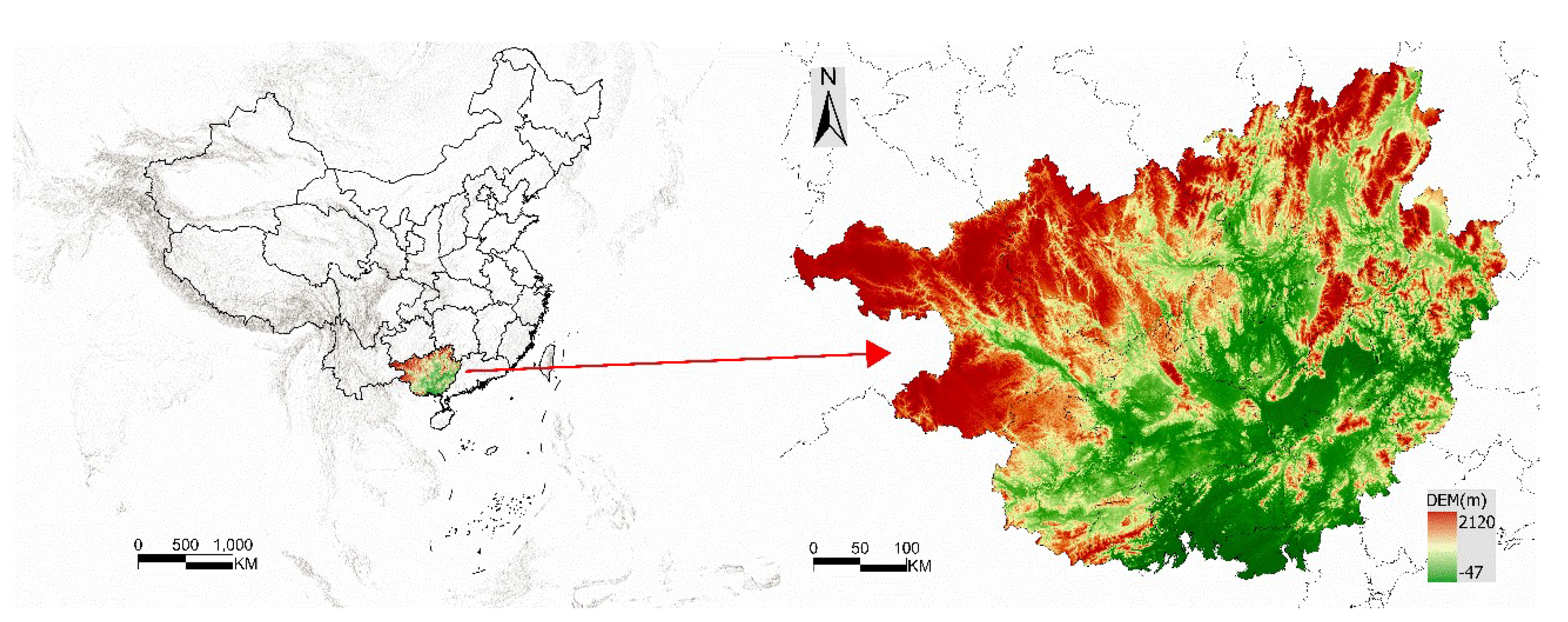
Figure 2.
Technical workflow.
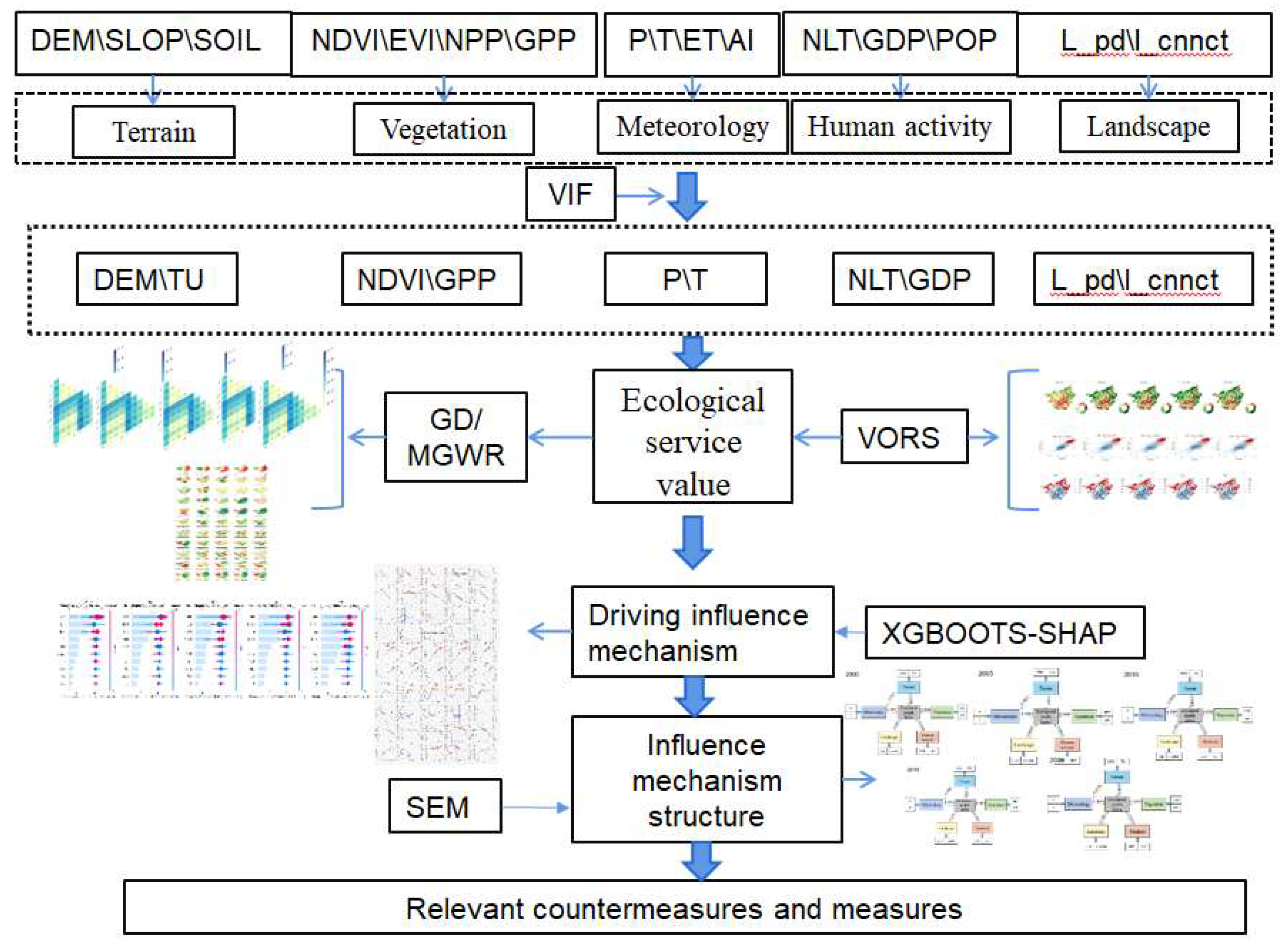
Figure 3.
Spatial evolution of ecosystem health from 2000 to 2020.
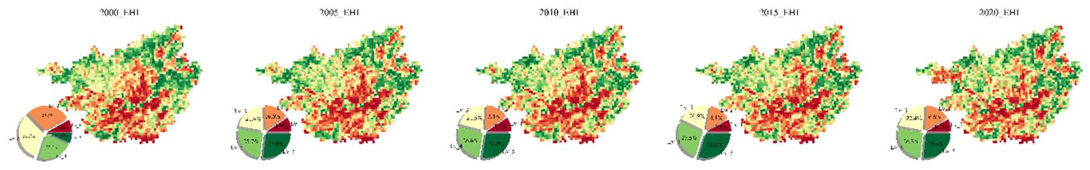
Figure 4.
The Moran Index of ecosystem health in Guangxi from 2000 to 2020.
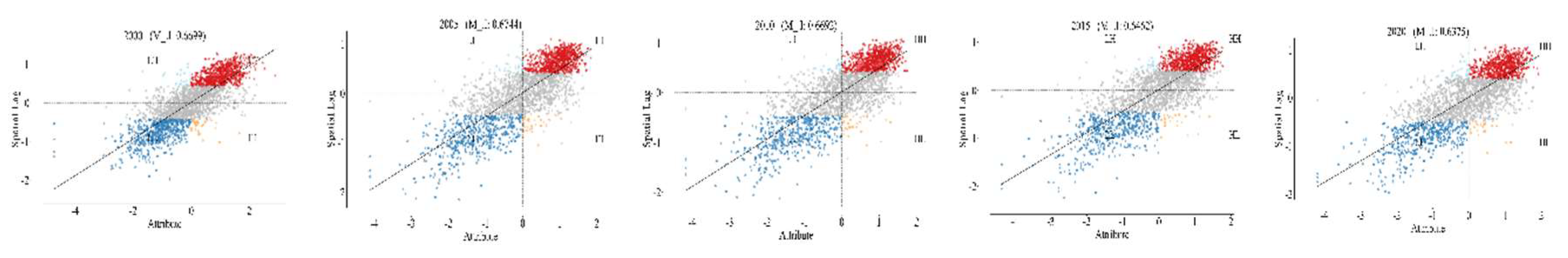
Figure 5.
Evolution space of ecosystem health agglomeration in Guangxi from 2000 to 2020.
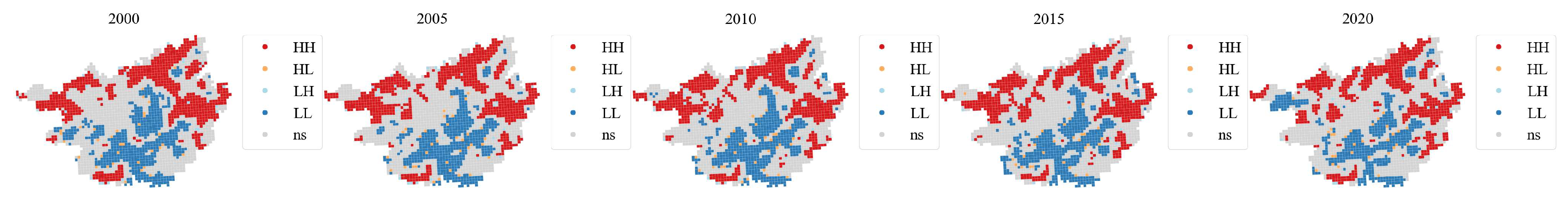
Figure 6.
Impacts of driving factors and interactions on ecosystem health from 2000 to 2020.
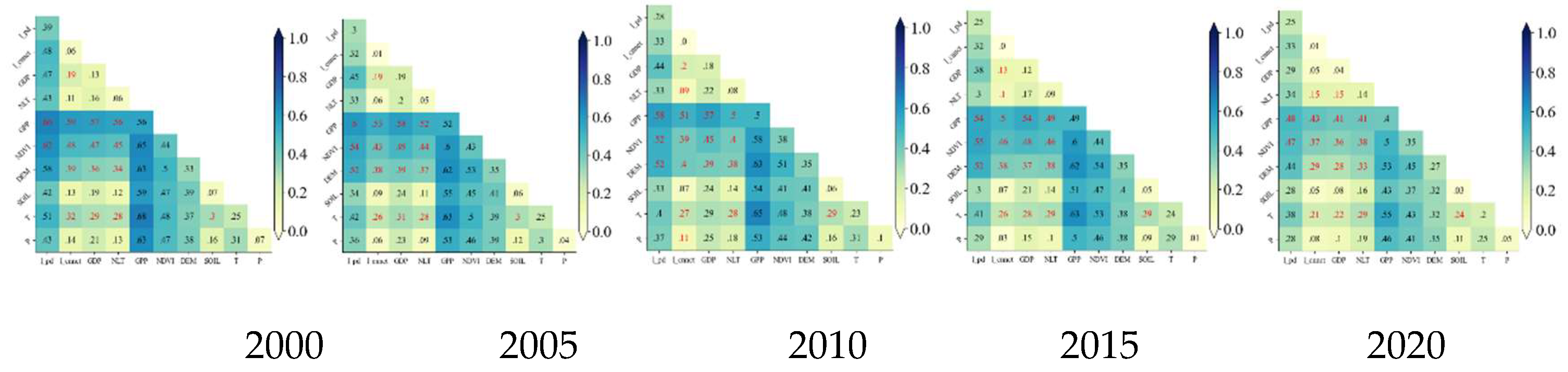
Figure 7.
The coefficients of MGWR model from 2000 to 2020.
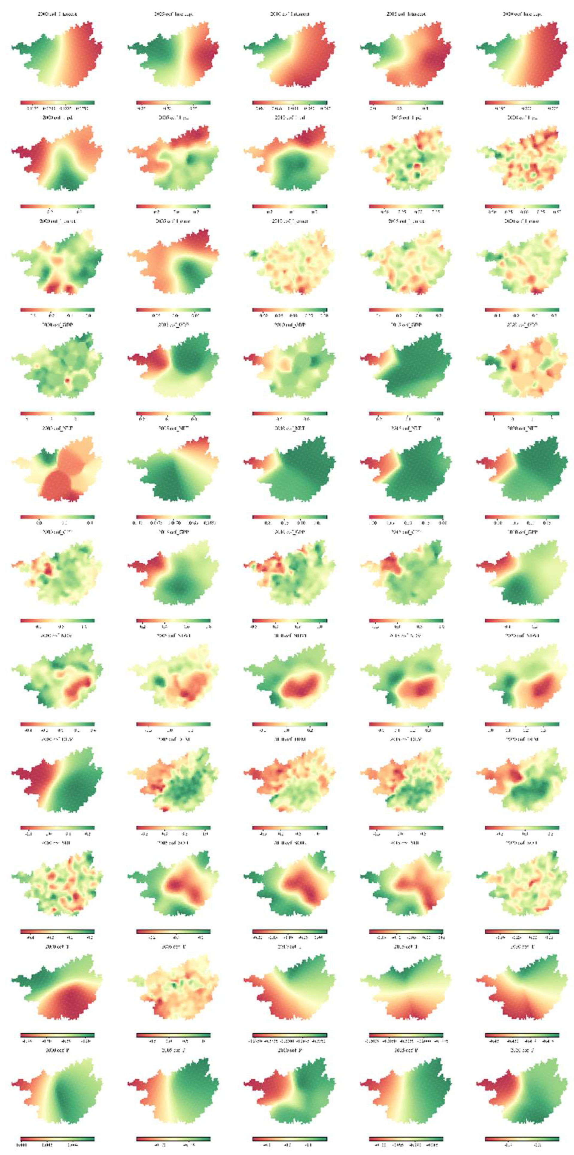
Figure 8.
The changes in the ordering of characteristics of driving factors from 2000 to 2020.
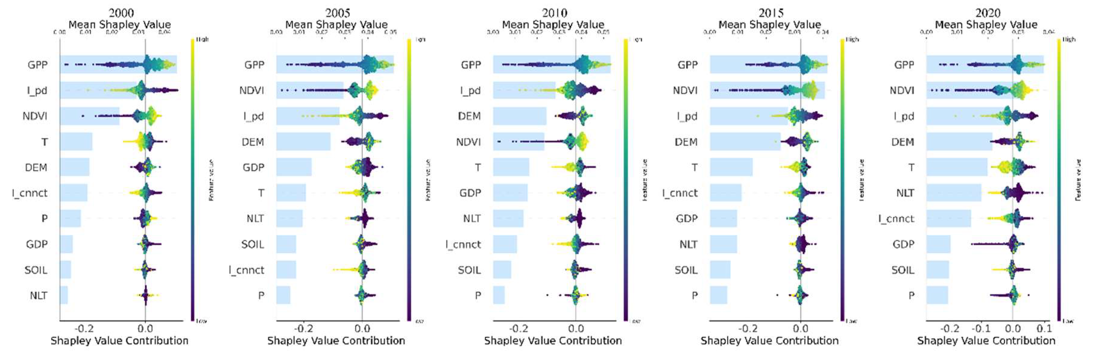
Figure 9.
The driving factors influence the critical value change from 2000 to 2020.
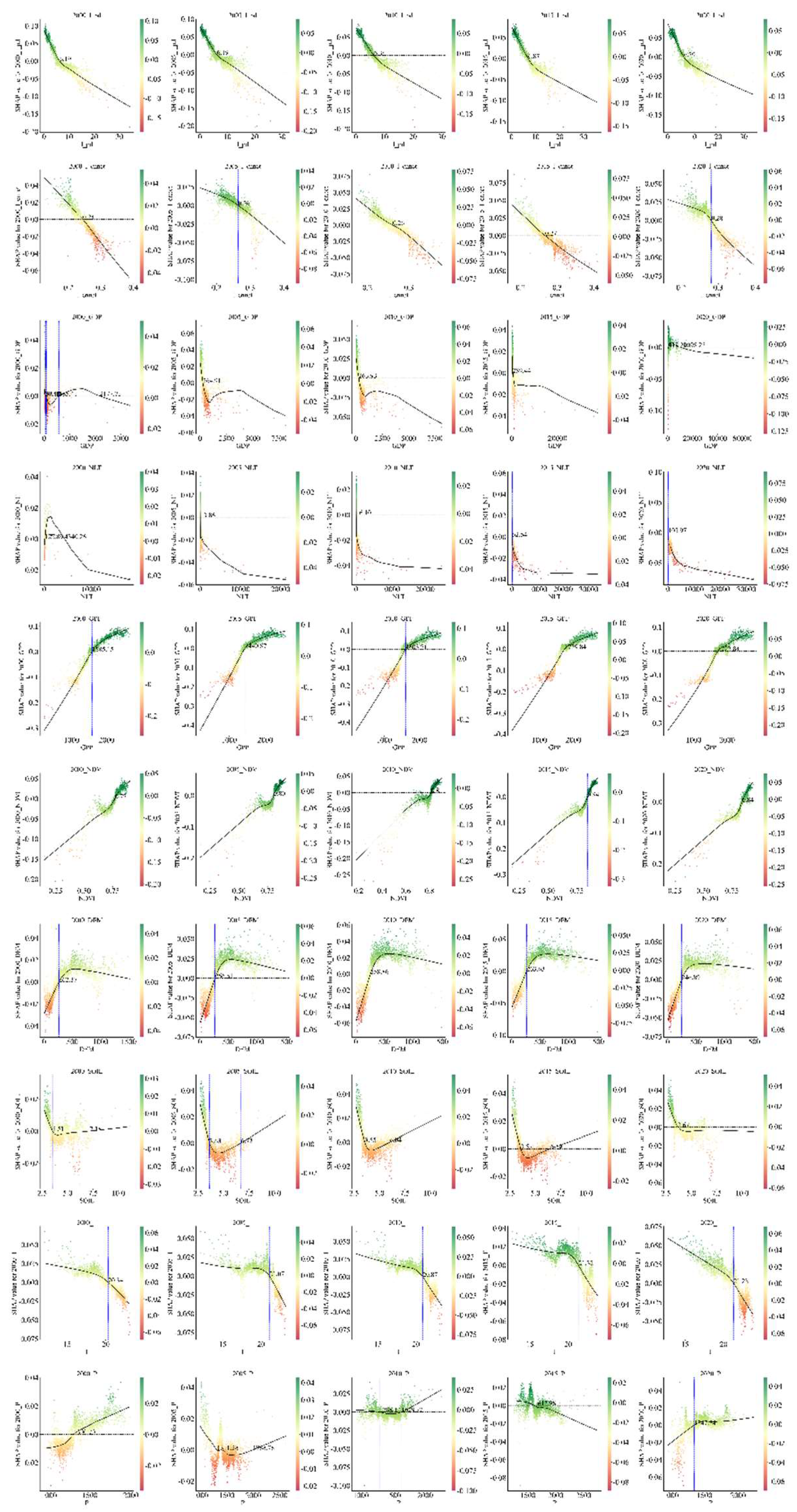
Figure 10.
Structure of influence of factors on ecosystem health.
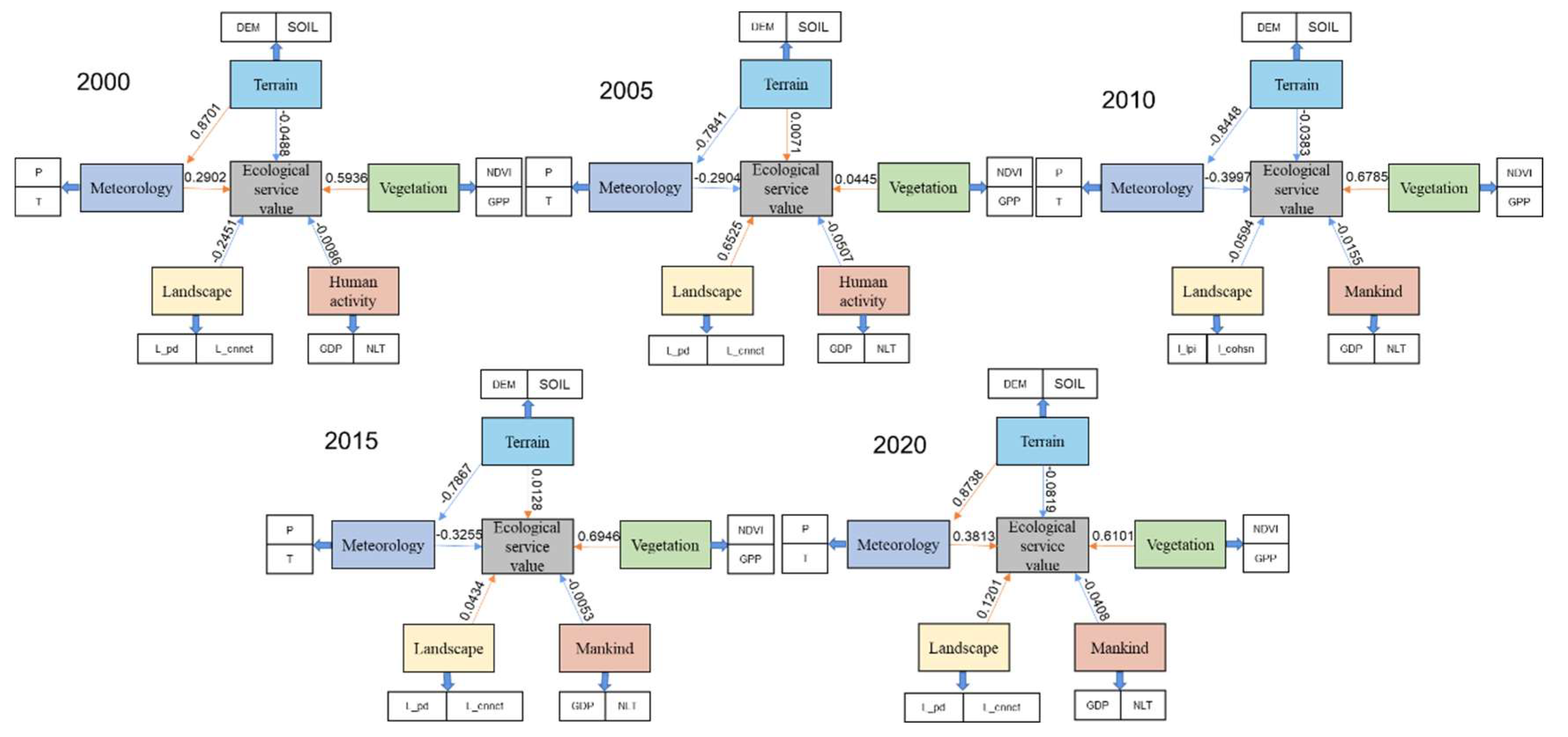

Table 1.
Indicators and data sources.
| Factor Type | Data Type | Data Description | Data Source |
| Ecology | Land utilization | 2000-2020 resolution 1km*1km | National Tibetan Plateau Scientific Data Center |
| NPP | Spatial resolution 500m*500m | Earth resource data cloud platform | |
| Vegetational type | China 1:1 million vegetation dataset | National Data Center for Glaciology and Permafrost Desert Science | |
| Agrotype | Spatial resolution 1km*1km | Resource Environmental Science and Data Center | |
| Terrain | DEM | Spatial resolution 450m | SRTM15 |
| Climate | Potential evapotranspiration | Spatial resolution 500m*500m | National Tibetan Plateau Scientific Data Center |
| Mean annual temperature | Spatial resolution 1km*1km | Resource Environmental Science and Data Center | |
| Human activity | Population | Spatial resolution 1km*1km | Resource Environmental Science and Data Center |
| Construction land | Spatial resolution 1km*1km | Resource Environmental Science and Data Center |
Table 2.
Variable declaration.
| Variable Abbreviation | Variable Name | Variable Description |
| GPP | Gross primary productivity | The total amount of carbon fixed by plants through photosynthesis per unit time, reflecting the primary productive capacity of the ecosystem (gC/m²•yr). |
| NDVI | Normalized difference vegetation index | The vegetation coverage index (range: -1~1) calculated based on the reflectance of red and near-infrared bands. The higher the value, the more dense the vegetation. |
| l_pd | Landscape patch density | The number of landscape patches per unit area (unit: units /km²), which represents the degree of landscape fragmentation (the higher the value, the more severe the fragmentation). |
| l_cnnct | Landscape connectivity | Describes the spatial connectivity between patches in a landscape (common index: probabilistic connectivity index) that affects species dispersal and ecological processes. |
| DEM | Digital elevation model | Digital representation of surface elevation (in meters) used to analyze topographic features such as slope and slope direction and their impact on ecological processes. |
| SOIL | Soil organic matter content | Soil key attributes (such as organic matter content, pH, texture, etc.), directly affecting vegetation growth and nutrient cycling. |
| GDP | Gross domestic product | Regional economic aggregate index (unit: yuan/person), reflecting the intensity of human economic activities and their pressure on the ecosystem. |
| NLT | Nighttime light | Night light brightness based on satellite remote sensing as an indicator of human activity intensity. |
| P | Precipitation | The total amount of precipitation per unit time (unit: mm) affects the water budget and vegetation distribution pattern of ecosystem. |
| T | Temperature | Temperature index (unit: ℃), regulating plant photosynthesis, respiration and species distribution. |
Table 3.
The comparison of GWR and MGWR model fit from 2000 to 2020.
| 2000 | 2005 | 2010 | 2015 | 2020 | ||||||
| GWR | MGWR | GWR | MGWR | GWR | MGWR | GWR | MGWR | GWR | MGWR | |
| AIC: | 3234.86 | 1915.94 | 3926.00 | 2311.69 | 3815.37 | 2306.74 | 3576.94 | 2252.14 | 4086.72 | 2591.34 |
| AICc: | 3236.99 | 2050.59 | 3928.13 | 2410.94 | 3817.50 | 2458.77 | 3579.07 | 2392.13 | 4088.86 | 2758.86 |
| BIC: | -17819.20 | 4033.76 | -17637.28 | 4151.23 | -17670.08 | 4545.46 | -17735.77 | 4407.98 | -17586.83 | 4931.04 |
| R2 | 0.77 | 0.90 | 0.70 | 0.88 | 0.71 | 0.89 | 0.74 | 0.89 | 0.68 | 0.88 |
| Ad. R2 | 0.77 | 0.89 | 0.70 | 0.86 | 0.71 | 0.87 | 0.74 | 0.87 | 0.67 | 0.85 |
Disclaimer/Publisher’s Note: The statements, opinions and data contained in all publications are solely those of the individual author(s) and contributor(s) and not of MDPI and/or the editor(s). MDPI and/or the editor(s) disclaim responsibility for any injury to people or property resulting from any ideas, methods, instructions or products referred to in the content. |
© 2025 by the authors. Licensee MDPI, Basel, Switzerland. This article is an open access article distributed under the terms and conditions of the Creative Commons Attribution (CC BY) license (http://creativecommons.org/licenses/by/4.0/).
Copyright: This open access article is published under a Creative Commons CC BY 4.0 license, which permit the free download, distribution, and reuse, provided that the author and preprint are cited in any reuse.


